Non-Parametric Model-Based Estimation of the Effective Reproduction Number for SARS-CoV-2 ^†

Abstract

Describing viral outbreaks, such as the COVID-19 pandemic, often involves employing compartmental models composed of ordinary differential equation (ODE) systems. Estimating the parameter values for these ODE models is crucial and relies on accessible data. To accurately represent realistic pandemic scenarios with diverse situations, it is necessary to consider model parameters as time dependent. However, estimating such time-dependent parameters, like transition rates in compartmental models, is notoriously challenging due to the unknown function class of these parameters. In this study, we propose a novel approach by using an Augmented Kalman Smoother (AKS) combined with an Expectation-Maximization (EM) algorithm to simultaneously estimate all time-dependent parameters in an SIRD compartmental model. Our approach can be applied to general ODE systems with time-varying parameters, requiring no prior knowledge of model parameters or additional assumptions on the function class of the ODE time dependencies. A key advantage of our method compared to other methods is that it does not require assumptions about the parameterization of the serial interval distribution for estimating SIRD model parameters. Applying our approach to COVID-19 data in Germany, we adequately describe time-series data with strong fluctuations and multiple waves, obtaining non-parametric model-based time-course estimates for the effective reproduction number.

1. Introduction

The last five decades have witnessed a significant rise in emerging infectious diseases, particularly zoonoses and vector-borne diseases [1,2]. To gain a comprehensive understanding of their dynamics, mathematical models have become an indispensable tool [3,4,5,6,7]. The global pandemic caused by the novel SARS-CoV-2 in 2020/21 prompted numerous modeling efforts, ranging from early situation assessments [8,9,10] to evaluating the effectiveness of non-pharmaceutical interventions [11,12,13], analyzing undetected cases [14,15] and employing agent-based model descriptions [16,17,18].

Infectious disease spread is often described by using the classical susceptible–infected–recovered (SIR) compartmental model where the model parameters are estimated from the observed data [19,20,21]. These parameters, specific to each disease, depend on the pathogen’s characteristics and its contagiousness [6,22]. To improve the description of infection dynamics, extensions to the classical SIR structure have been proposed, including differentiation between deceased (D) and recovered (R) individuals or the introduction of an intermediate exposed compartment (E) for infected but not yet contagious individuals. While more compartments can offer detailed descriptions, overly complex models may face challenges in parameter estimation due to limited data availability and parameter identifiability issues [23]. Nevertheless, comprehensive SIR-like model structures have been developed for COVID-19, covering essential features like asymptomatic infectious individuals, undetected infections and different hospitalization states [8,24,25,26,27].

The temporal variations in detected SARS-CoV-2 infection case numbers, with multiple epidemic waves observed in most countries [28,29], necessitate time-dependent model parameters to accurately describe the dynamics [30,31,32]. Time dependencies in the parameters account for seasonal effects [33,34] and changes in population behavior or the impact of non-pharmaceutical interventions. Among the various model parameters of interest, the effective reproduction number ${\mathcal{R}}_t$ holds particular significance in epidemic models. It represents the average number of secondary infections caused by one infectious individual and varies over time, offering insight into the outbreak’s current status and indicating turning points in infection growth. Estimating the effective reproduction number from measured data via epidemic models with time-dependent parameters has been a key focus for informing governmental decision makers during the SARS-CoV-2 pandemic. Different approaches have been proposed, such as specifying step functions to incorporate non-pharmaceutical interventions [9] or assuming spline functions to capture flexible time dependencies [35]. While these approaches offer valuable insights into pandemic scenarios, they depend on the selected function class and often require a high number of model parameters, leading to challenges in parameter estimation. Defining functions to adequately represent more diffuse changes, such as behavioral adjustments in the population, remains challenging.

Addressing the task of estimating time-dependent parameters in high-dimensional ordinary differential equation (ODE) models, especially with sparse data, poses difficulties [36,37,38,39]. In the field of epidemiology, established methods like Sequential Monte Carlo (SMC) or particle Markov chain Monte Carlo (pMCMC) have been successfully applied to estimate time-dependent transmission rates in SIR-type models [40,41,42,43,44,45]. However, these methods often require the careful calibration of meta parameters and can be computationally expensive. Alternatively, function-class-free methods, like iterative Kalman-filter-based approaches, offer computationally simpler and cheaper alternatives [46].

In this study, we present a function-class-free approach that simultaneously estimates the time dependencies of all the dynamical parameters in the state-space representation of an SIRD model, including the effective reproduction number. We employ the Ensemble or Augmented Kalman Smoother (AKS) method, treating dynamic parameters as states to estimate their time dependencies [47]. Unlike recent approaches that use the Augmented Kalman Filter for estimating the time-dependent reproduction number in COVID-19 data [48] based on “trial and error”, our method combines the Augmented Kalman Smoother with an Expectation-Maximization (EM) algorithm [49,50]. Notably, we demonstrate that our approach is capable of describing real-world COVID-19 data while providing time-dependent estimates for all the model parameters. Importantly, our method requires no additional prior knowledge about the remaining model parameters, total population numbers or initial values of individual compartments. We apply this algorithm to SARS-CoV-2 incidence data in Germany from winter 2020 to summer 2021, obtaining time-dependent estimates for all the model parameters and real-time estimates of the effective reproduction number ${\mathcal{R}}_t$.

The code for the AKS method and the analysis scripts used in this work are freely available on GitHub at https://github.com/vandensich/Augmented-Kalman-Smoother (release v1.0, published on 14 November 2023) and are published under the MIT license.

This work extends a previously published conference paper that addresses the same scientific core content [51]. The introduction and methods sections have been rephrased, and two substantial parts have been added. Section 3.1, Section 3.2 and Section 3.3 present the results of an extensive simulation study, analyzing the method’s performance on generated data sets. Additionally, Section 3.5 and Section 5 include the results of a successful validation, where the estimated parameter time courses were used as inputs for an ODE model predicting the model states.

2. Materials and Methods

2.1. SIRD Model and Reparameterization

The conventional method of characterizing the propagation of an infectious disease within a population involves employing the SIR model [20]. This model comprises three compartments: susceptible S, infected I and removed R. Frequently, the removed compartment is further divided into recovered R and deceased D, leading to the SIRD model [52]. The time-continuous evolution of this model is described by the following system of ODEs:

$$\begin{array}{c}\hfill \begin{array}{cc}\hfill \dot{S}& =-\beta ·\frac{S·I}{N_0}\hfill \\ \hfill \dot{I}& =\beta ·\frac{S·I}{N_0}-\gamma ·I-\theta ·I\hfill \\ \hfill \dot{R}& =\gamma ·I\hfill \\ \hfill \dot{D}& =\theta ·I.\hfill \end{array}\end{array}$$

(1)

The model contains three time-constant transition rate parameters: $\beta$, $\gamma$ and $\theta$, which represent the infection rate, recovery rate and mortality rate, respectively. Initially, at $t=0$, the values of the four compartments are denoted as $S\left(0\right)=S_0$, $I\left(0\right)=I_0$, while $R\left(0\right)=0$ and $D\left(0\right)=0$, ensuring that the total number of individuals is given by $N_0=S_0+I_0$.

In the early stages of an epidemic, when $S_0\approx N_0$, the disease-specific basic reproduction number denoted as ${\mathcal{R}}_0$, which represents the average number of secondary cases, can be directly calculated from the model parameters as ${\mathcal{R}}_0=\beta /(\gamma +\theta )$. As the disease spreads and more individuals become infected, the assumption $S\left(t\right)\approx N_0$ is no longer valid, and the time-dependent effective reproduction number is defined in the literature as [53]

$$\begin{array}{cc}\hfill {\mathcal{R}}_t^{\ast }& =\frac{\beta }{\gamma +\theta }·\frac{S\left(t\right)}{N_0}\hfill \end{array}$$

(2)

which depends on the change in the susceptible individuals $S\left(t\right)$ over time. The effective reproduction number ${\mathcal{R}}_t^{\ast }$ serves as a crucial metric for understanding the status of an epidemic, where ${\mathcal{R}}_t^{\ast }>1$ indicates an increasing number of newly infected individuals and ${\mathcal{R}}_t^{\ast }<1$ suggests a declining trend.

In addition to intrinsic factors, external influences such as seasonal variations and behavioral changes in the population significantly impact viral transmission. The time dependencies in the infection rate $\beta$ effectively capture the influence of increased hygiene standards and non-pharmaceutical interventions, which play a critical role in epidemic development. The manifestation of such effects can be observed through the emergence of epidemic scenarios featuring multiple waves of infections, as seen in seasonal influenza and COVID-19 outbreaks. To accommodate the dynamic nature of epidemics, an unambiguous model extension involves considering time-dependent transition rates: ${\beta }_t$, ${\gamma }_t$ and ${\theta }_t$. By incorporating these temporal changes into the model, we can accurately define the effective reproduction number within the context of evolving epidemic patterns as

$$\begin{array}{cc}\hfill {\mathcal{R}}_t& =\frac{{\beta }_t}{{\gamma }_t+{\theta }_t}·\frac{S\left(t\right)}{N_0}.\hfill \end{array}$$

(3)

In order to simplify the estimation of ${\mathcal{R}}_t$, we substitute Equation (3) into Equation (1), yielding a reparameterized version of the SIRD model:

$$\begin{array}{c}\hfill \begin{array}{cc}\hfill \dot{S}& =-{\mathcal{R}}_t·({\gamma }_t+{\theta }_t)·I\hfill \\ \hfill \dot{I}& =({\mathcal{R}}_t-1)·({\gamma }_t+{\theta }_t)·I\hfill \\ \hfill \dot{R}& ={\gamma }_t·I\hfill \\ \hfill \dot{D}& ={\theta }_t·I.\hfill \end{array}\end{array}$$

(4)

It is important to highlight that as a result of this transformation, the susceptible compartment S no longer appears on the right-hand side of Equation (4). Consequently, the differential equation for S can be disregarded without impacting the solution of the remaining system.

Parameter estimation for non-linear ODE models with time-constant parameters typically involves the utilization of efficient numerical optimization algorithms. These algorithms aim to minimize the difference between recorded data and model trajectories by adjusting parameter values, often employing maximum-likelihood estimation techniques [54,55,56,57,58]. However, in the context of changing transmission rates during an infectious disease outbreak, the time dependency of the model parameters is unknown and needs to be estimated from the data as well. This estimation task, known as input estimation for ODE models, presents challenges as existing methods are often limited by their assumptions of specific function classes for time-dependent model parameters, such as step functions, splines or combinations of sustained and transient-response functions [39,59]. In contrast, we propose a function-class-free approach based on Kalman Filter and Smoother methods. This approach enables the estimation of dynamics for unobserved model states and, with appropriate extensions, also facilitates the estimation of time dependencies in the model parameters.

2.2. Estimation of Time-Dependent Parameters in Non-Linear ODE Models via the Augmented Kalman Smoother

The Kalman Filter is an iterative algorithm commonly used to estimate the time courses of unobserved states within a linear model by utilizing noisy observations collected over time. Alongside the Kalman Filter, the Kalman Smoother is a two-step algorithm involving a forward pass with the Kalman Filter followed by a backward-pass procedure of a similar nature. In scenarios involving non-linear models, the Extended Kalman Filter and Smoother are applied to linearize such models incrementally, enabling analysis. For the examination of time-varying parameters in non-linear models, the Augmented Kalman Smoother (AKS) serves as a notable approach. The AKS combines the Extended Kalman Smoother with the capability to consider time-dependent parameters.

2.2.1. State-Space Model

The Kalman Filter and its extensions operate in the time-discrete state-space representation of a particular model. It is given by the general form

$$\begin{array}{c}\hfill \begin{array}{cc}\hfill x_{k+1}& =b\left(x_k\right)+{ϵ}_k\hfill \\ \hfill y_k& =H·x_k+{\eta }_k,\hfill \end{array}\end{array}$$

(5)

for discrete time points k of the n-dimensional process state vector $x_k$ and the d-dimensional vector of observables $y_k$, where $n>d$. The transition of the state vector x, from time point k to time point $k+1$, is determined by applying the transition function b. This process incorporates additive Gaussian noise, ${ϵ}_k\sim \mathcal{N}(0,Q)$, which follows a normal distribution with a mean of zero and covariance matrix Q, to account for process noise. Since not all states are directly observable, the observation matrix H establishes the relationship between the state vector x and the observable vector y. Similarly, the observations $y_k$ are subject to additive Gaussian noise, ${\eta }_k\sim \mathcal{N}(0,M)$, with a covariance matrix M, representing the measurement noise.

The structure of a given ODE model, represented as $\dot{x}=f(x,p)$, where x denotes the states and p represents m parameters, can be transformed into its discrete state-space formulation. In this formulation, the solutions of the ODE correspond to the states x in the state space and the right-hand side f of the ODE is translated into time-discrete update rules, which are represented by the transition function b. In addition, the observation matrix H needs to be specified in the state-space formulation, defining the relationship between the data vector y and the corresponding states in the state vector x.

2.2.2. Augmented Kalman Smoother

To estimate the unobserved process states in the state-space model represented by Equation (5), particularly for non-linear models, the Extended Kalman Smoother (EKS) is employed [60]. The EKS assumes time-constant parameters and necessitates input values for all model parameters.

For the estimation of the time-dependent parameters, we introduce an extension of the Extended Kalman Filter and Smoother algorithms, which we refer to as the Augmented Kalman Smoother (AKS), following the principles of the previously published Augmented Kalman Filter [61,62]. The AKS formulation closely resembles that of the EKS, but with a key difference: it introduces additional process states for each time-dependent model parameter. Consequently, the AKS only requires appropriate initial values for those states and parameters that vary over time.

As a result of this enhancement, the AKS provides estimates not only for the time courses of unobserved process states but also for the time courses of the time-dependent model parameters. Furthermore, the AKS method simultaneously estimates the covariance matrices P of the state-space vector x of the analyzed process. The algorithm is initialized at time point $k=1$, where the process-state vector $x_0$ and the process-state covariance matrix $P_0$ at time point $k=0$ are provided as inputs for the iterations.

The first step of the algorithm is the so-called prediction step

$$\begin{array}{cc}\hfill x_{k|k-1}& =b\left(x_{k-1|k-1}\right)\hfill \end{array}$$

(6)

$$\begin{array}{cc}\hfill P_{k|k-1}& =F_k·P_{k-1|k-1}·F_k^{\mathrm{T}}+Q.\hfill \end{array}$$

(7)

Here, $x_{k|k-1}$ and $P_{k|k-1}$ represent the predicted state vector and covariance matrix at time k, respectively, based on the $k-1$ previous data points. The initial predicted state vector $x_{1|0}$ is computed by applying the transition function b to the state vector $x_0$. During the step-wise linearization process, the Jacobian of b at the point $x_{k-1|k-1}$ is calculated as

$$\begin{array}{cc}\hfill F_k& =\frac{\partial b}{\partial x}{|}_{x_{k-1|k-1}}.\hfill \end{array}$$

(8)

The second step of the algorithm is the update step, where the predicted state vector and covariance matrix are updated by using the noisy measurement $y_k$:

$$\begin{array}{cc}\hfill K_k& =P_{k|k-1}·H_k^{\mathrm{T}}·{\left(H_k·P_{k|k-1}·H_k^{\mathrm{T}}+M\right)}^{-1}\hfill \end{array}$$

(9)

$$\begin{array}{cc}\hfill x_{k|k}& =x_{k|k-1}+K_k·\left(y_k-H_k·x_{k|k-1}\right)\hfill \end{array}$$

(10)

$$\begin{array}{cc}\hfill P_{k|k}& =P_{k|k-1}-K_k·H_k·P_{k|k-1}\hfill \end{array}$$

(11)

The Kalman gain, denoted as $K_k$, is obtained via Equation (9), utilizing the measurement covariance matrix M and the predicted covariance matrix $P_{k|k-1}$ of the process. It represents the relative weight between the noisy measurements and the model predictions, where a larger Kalman gain implies that more emphasis is placed on the measurements for the next prediction step. This effectively balances the uncertainties of the model predictions and the measurement uncertainties, enabling adaptive updates. The predictions are subsequently updated according to Equations (10) and (11), completing one iteration of the algorithm. The updated state vector $xk|k$ and the updated covariance matrix $Pk|k$ are then used as inputs for the following prediction step. This iterative process is repeated until all the observed time points have been considered.

The filter, defined by Equations (6)–(11), performs forward estimation of the state-space vector x and its covariance matrix P. A limitation of this filtering method is that the estimate $x_{k|k}$ is only based on the $k-1$ previous data points, resulting in estimates at the beginning of the time series being less informed than those at the end. Furthermore, the estimates of the filter always lag one step behind the data. To address this issue, the filter is commonly combined with a smoother, resulting in a Rauch–Tung–Striebel Smoother [63]. The smoother runs backward from $k=N-1$ to $k=0$, initialized with the last updated estimates of the filter $x_{N|N}$ and $P_{N|N}$. It leverages the noisy measurements $y_k$ indirectly by comparing the estimates and predictions generated by the filter. This process generates smoothed estimates at each time point k, incorporating all the available data:

$$\begin{array}{cc}\hfill B_k& =P_{k|k}·F_k^{\mathrm{T}}·P_{k+1|k}^{-1}\hfill \end{array}$$

(12)

$$\begin{array}{cc}\hfill x_{k|N}& =x_{k|k}+B_k·\left(x_{k+1|N}-x_{k+1|k}\right)\hfill \end{array}$$

(13)

$$\begin{array}{cc}\hfill P_{k|N}& =P_{k|k}+B_k·\left(P_{k+1|N}-P_{k+1|k}\right)·B_k^{\mathrm{T}},\hfill \end{array}$$

(14)

and thereby improving the accuracy of the estimates and mitigating the lagging issue of the filter. Here, $B_k$ is the smoother gain that is similar in function to the Kalman gain $K_k$ in Equation (9). As a final result, the AKS algorithm yields the state covariance matrices $P_{k|N}$ and the smoothed estimates for the state vector $x_{k|N}$ that represents the trajectories of the model states as well as the time courses of the model parameters.

2.2.3. Expectation-Maximization Algorithm for AKS Initial Parameters

To ensure the effective operation of a Kalman Smoother algorithm, appropriate initial values for $x_0$, $P_0$, Q and M need to be provided. To achieve optimal starting conditions, an Expectation-Maximization (EM) algorithm can be employed. Its expectation step (E-step) consists of the AKS algorithms. Using the smoothed estimates $x_{k|N}$ and $P_{k|N}$, a maximum-likelihood estimation is carried out for the covariance matrices Q and M. This involves determining update equations for Q and M by maximizing the following target function [64] with respect to these matrices:

$$\begin{array}{c}\hfill \begin{array}{cc}\hfill L=& -\frac{1}{2}ln\left|P_0\right|-\frac{1}{2}\mathrm{Tr}\left[P_0^{-1}{P}_{0|N}\right]-\frac{N}{2}ln\left|Q\right|-\frac{1}{2}\mathrm{Tr}\left[Q^{-1}\sum _{k=1}^N{\Sigma }_k\right]\hfill \\ \hfill & -\frac{N}{2}ln\left|M\right|-\frac{1}{2}\mathrm{Tr}\left[M^{-1}\sum _{k=1}^N{\Omega }_k\right]\hfill \\ \hfill \mathrm{where}{\Sigma }_k=& P_{k|N}+(x_{k|N}-b\left(x_{k-1|N}\right))·{(x_{k|N}-b\left(x_{k-1|N}\right))}^{\mathrm{T}}\hfill \\ \hfill & +F_k·P_{k-1|N}·F_k^{\mathrm{T}}-P_{k-1,k|N}·F_k^{\mathrm{T}}-F_k·P_{k-1,k|N}^{\mathrm{T}}\hfill \\ \hfill {\Omega }_k=& (y_k-G·x_{k|N})·{(y_k-G·{\mathbf{x}}_{k|N})}^{\mathrm{T}}+G·P_{k|N}·G^{\mathrm{T}}\hfill \end{array}\end{array}$$

(15)

Analytically, it can be shown that the maximum is reached for

$$\begin{array}{c}\hfill Q_{\mathrm{new}}=\frac{1}{N}\sum _{k=1}^N{\Sigma }_k\mathrm{and}{M}_{\mathrm{new}}=\frac{1}{N}\sum _{k=1}^N{\Omega }_k,\end{array}$$

(16)

which then serve as the input for the next EM iteration [64]. Furthermore, the values for $x_{0|N}$ and $P_{0|N}$ obtained via the AKS from the previous iteration are used as the initial values $x_0$ and $P_0$ for the next iteration, which corresponds to the maximization step (M-step) of the EM algorithm. These iterative steps are repeated until a chosen convergence criterion reaches a certain level $\alpha$:

$$\begin{array}{c}\hfill \frac{\left|\left({\displaystyle {\displaystyle \sum _i}}{Q}_i+{\displaystyle \sum _i}{M}_i+{\displaystyle \sum _i}{x}_{0,i}+{\displaystyle \sum _i}{P}_{0,i}\right)-\left({\displaystyle \sum _i}{Q}_{\mathrm{new},i}+{\displaystyle \sum _i}{M}_{\mathrm{new},i}+{\displaystyle \sum _i}{x}_{0|N,i}+{\displaystyle \sum _i}{P}_{0|N,i}\right)\right|}{\left|\left({\displaystyle \sum _i}{Q}_i+{\displaystyle \sum _i}{M}_i+{\displaystyle \sum _i}{x}_{0,i}+{\displaystyle \sum _i}{P}_{0,i}\right)\right|}<\alpha \end{array}$$

(17)

Here, $\alpha$ denotes the relative tolerance for the difference between the consecutive hyperparameter estimates Q, M, $x_0$ and $P_0$. The iteration process continues until the relative difference between the consecutive hyperparameter estimates falls below the tolerance level $\alpha$. In the combined application of the AKS, it is necessary to provide an initial guess for these hyperparameters to start the EM algorithm. However, the presented analyses indicate that the choice of these initial values is not crucial for achieving high-quality final results. A visualization of the method in the form of pseudo code is shown in Algorithm 1.

Algorithm 1 Augmented Kalman Smoother (AKS)
1:	procedure AKS($Raw\_data$)
2:	▹Data processing
3:	$data\leftarrow Raw\_data$
4:	▹ Model parameters and initial values
5:	$G\leftarrow$ observation_matrix()
6:	$x0\leftarrow$ initial_state_vector_guess()
7:	$u0\leftarrow$ initial_state_covariance_guess()
8:	$P0\leftarrow$initialize_state_covariance($u0$)
9:	$Q\leftarrow$ initial_evolution_error_guess()
10:	$M\leftarrow$ initial_observation_error_guess()
11:	▹AKS initialization
12:	$x\leftarrow x0$
13:	$P\leftarrow P0$
14:	$count\leftarrow 0$
15:	$ϵ\leftarrow 100$
16:	▹Main loop for AKS
17:	while $ϵ>1e-3$ do
18:	▹ Predict state-space vectors and covariance matrices
19:	$Pred,P\_Pred\leftarrow$ AKF_Prediction($x,P,Q$)	[Equations (6)–(8)]
20:	▹Filter state-space vectors and covariance matrices
21:	$Est,P\_Est,Gain,P\_lag,Jacob\leftarrow$ AKF_Update($data,G,Pred,P\_Pred,M$)	[Equations (9)–(11)]
22:	▹ Smooth state-space vectors and covariance matrices
23:	$smooth,std,P\_smooth,B\_list\leftarrow$ AKS_Smoother($Est,P\_Est,Gain,P\_lag,Jacob$)	[Equations (12)–(14)]
24:	▹Perform M-step for parameter estimation
25:	$M,Q,x0,P0\leftarrow$ M_step($data,Pred,P\_Pred,Jacob,P\_Est,P\_smooth,B\_list$)	[Equations (15) and (16)]
26:	▹Update AKS variables
27:	$x,P,count\leftarrow$ update_AKS_variables($smooth\_list,P\_smooth,x0,P0,count$)
28:	▹Check convergence criterion
29:	$ϵ\leftarrow$ check_convergence($P,x,Q,M,x0,P0$)	[Equation (17)]
30:	end while
31:	▹Return results
32:	return smoothed_results
33:	end procedure

2.2.4. From the Time-Continuous ODE System to Its Time-Discrete State-Space Formulation

Although we apply the presented Kalman Smoother method exclusively to epidemic models within this paper, it is in general applicable to any partially observed non-linear ODE systems, as is shortly outlined in the following. Let us consider the following time-continuous dynamic ODE model:

$$\begin{array}{cc}\hfill \dot{x}& =f(x,p).\hfill \end{array}$$

(18)

In the time-discrete formalism, the time derivative of the state variables x is represented by a function f that depends on both the state vector itself and the parameter vector p. Additionally, the initial conditions of the ODE system can also be regarded as parameters within p.

For the time-discrete formulation, the right-hand side of the ODE, denoted as $f(x,p)$, is interpreted as an update equation for each discrete time step, transitioning from $x_{k-1}$ to $x_k$. Consequently, Equation (18) can be expressed as

$$\left(\begin{array}{c}{x}_k\\ p_k\end{array}\right)=\left(\begin{array}{c}{x}_{k-1}\\ p_{k-1}\end{array}\right)+\left(\begin{array}{c}f(x_{k-1},p_{k-1})\\ 0\end{array}\right)+{ϵ}_{k-1}.$$

(19)

The parameters $p_k$ are considered as supplementary states in the state space and are not updated according to the ODE model structure, as indicated by the zero term in the equation. Instead, their time dependence solely arises from the additive noise term ${ϵ}_{k-1}$, which is simultaneously estimated by the Kalman Smoother at each step. This additional degree of freedom grants the Kalman-Smoother-based approach the ability to adapt these parameters based on the available data. Consequently, the approach achieves a data-driven estimation of time-dependent parameters in an ODE system without any constraints on the parameters’ trajectory.

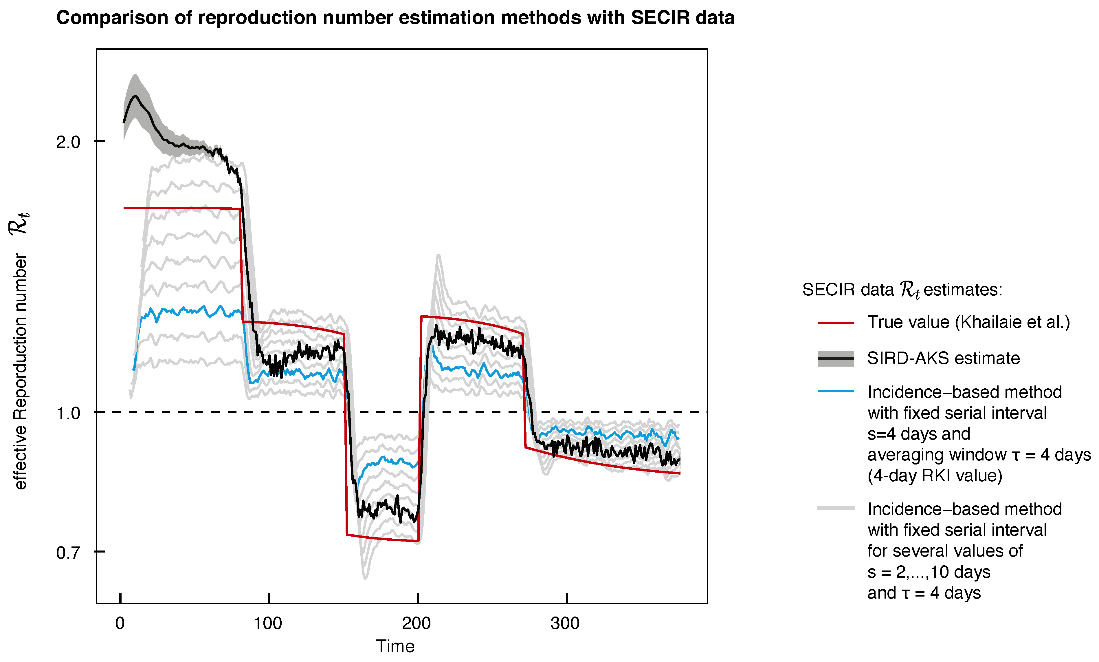
2.3. SIRD-AKS Method for Estimating the Effective Reproduction Number ${\mathcal{R}}_t$

Based on the general derivation in Equation (19), the time-discrete state-space formulation of the SIRD model from Equation (4) can be written as

$$\begin{array}{c}\hfill x_k=\left(\begin{array}{c}{S}_k\\ I_k\\ R_k\\ D_k\\ {\mathcal{R}}_k\\ {\gamma }_k\\ {\theta }_k\end{array}\right)=b\left(x_{k-1}\right)+{ϵ}_{k-1}=\left(\begin{array}{c}{S}_{k-1}\\ I_{k-1}\\ R_{k-1}\\ D_{k-1}\\ {\mathcal{R}}_{k-1}\\ {\gamma }_{k-1}\\ {\theta }_{k-1}\end{array}\right)+\left(\begin{array}{c}-{\mathcal{R}}_{k-1}·({\gamma }_{k-1}+{\theta }_{k-1})·I_{k-1}\\ ({\mathcal{R}}_{k-1}-1)·({\gamma }_{k-1}+{\theta }_{k-1})·I_{k-1}\\ {\gamma }_{k-1}·I_{k-1}\\ {\theta }_{k-1}·I_{k-1}\\ 0\\ 0\\ 0\end{array}\right)+{ϵ}_{k-1},\end{array}$$

(20)

where the first four rows are the four states of the time-continuous ODE and ${ϵ}_{k-1}$ corresponds to the process noise, as introduced in Equation (5). To incorporate the desired time dependence of the three SIRD model parameters, namely ${\mathcal{R}}_k$, ${\gamma }_k$ and ${\theta }_k$, the AKS method treats these parameters as additional states within the state-space formulation, leading to the SIRD-AKS model. As a result, the SIRD-AKS not only provides time-course estimates for the model states $S_k$, $I_k$, $R_k$ and $D_k$, but also for the parameters ${\mathcal{R}}_k$, ${\gamma }_k$ and ${\theta }_k$.

In real-world outbreak scenarios, data on the number of currently infectious individuals in state I per day are often unavailable. However, the incidence, representing the number of newly infected cases per time period, is commonly reported and easily accessible. In the SIRD model, these incidence numbers correspond to the flux of individuals into the infectious state, given by $v_{I,k}=\mathcal{R}k·(\gamma k+{\theta }_k)·I_k$, transitioning from time step k to $k+1$. Similarly, published data for the number of newly recovered $v_{R,k}={\gamma }_k·I_k$ and newly deceased $v_{D,k}={\theta }_k·I_k$ individuals form the fluxes into their respective states. Hence, the fluxes $v_{I,k}$, $v_{R,k}$ and $v_{D,k}$ serve as the observables $y_k$ for the SIRD-AKS method.

However, the observation matrix H introduced in Equation (5) only allows linear relationships between observables and states. To address this limitation and map the data to the appropriate variables of the state space for the SIRD-AKS method, the state-space formulation is expanded once more by introducing three additional states corresponding to the three fluxes, resulting in

$$\begin{array}{cc}\hfill x_k& =\left(\begin{array}{c}{S}_k\\ I_k\\ R_k\\ D_k\\ {\mathcal{R}}_k\\ {\gamma }_k\\ {\theta }_k\\ v_{I,k}\\ v_{R,k}\\ v_{D,k}\end{array}\right)=b\left(x_{k-1}\right)+{ϵ}_{k-1}=\left(\begin{array}{c}{S}_{k-1}\\ I_{k-1}\\ R_{k-1}\\ D_{k-1}\\ {\mathcal{R}}_{k-1}\\ {\gamma }_{k-1}\\ {\theta }_{k-1}\\ 0\\ 0\\ 0\end{array}\right)+\left(\begin{array}{c}-v_{I,k-1}\\ v_{I,k-1}-v_{R,k-1}-v_{D,k-1}\\ v_{R,k-1}\\ v_{D,k-1}\\ 0\\ 0\\ 0\\ {\mathcal{R}}_{k-1}·({\gamma }_{k-1}+{\theta }_{k-1})·I_{k-1}\\ {\gamma }_{k-1}·I_{k-1}\\ {\theta }_{k-1}·I_{k-1}\end{array}\right)+{ϵ}_{k-1}\hfill \end{array}$$

(21)

and an observation matrix

$$\begin{array}{cc}\hfill H& =\left(\begin{array}{cccc}& 1& 0& 0\\ 0_{M_{7\times 3}}& 0& 1& 0\\ & 0& 0& 1\end{array}\right).\hfill \end{array}$$

(22)

that links the incidence data to the respective fluxes $v_{I,k}$, $v_{R,k}$ and $v_{D,k}$. The SIRD-AKS method utilizes incidence data to estimate the state-space vector $x_k$ through the state-space formulation defined in Equation (21). The entries of $x_k$ are interpreted as discretized time series of the model states, time-dependent parameters and fluxes, i.e., incidence numbers. To ensure that all the variables remain strictly positive, the entire analysis is conducted on a logarithmic scale for $x_k$. Employing the logarithmic scale offers advantages in terms of numerical stability.

2.4. Incidence-Based Reproduction-Number-Calculation Method

In contrast to estimating the effective reproduction number ${\mathcal{R}}_t$ as a time-dependent parameter by using the SIRD-AKS method, it can also be calculated directly from incidence data based on the incidence-based method formulated in [65]. This method requires both incidence data and information about the empirical serial interval distribution, which represents the time period between the onset of illness in an infected case and the onset of illness in a subsequent case.

Due to the unavailability of reliable data on the serial interval distribution during the early stages of the SARS-CoV-2 pandemic, the German federal center for disease control and prevention (Robert Koch Institute or RKI) chose to use the incidence-based method from [65] and assumed a Dirac $\delta$-distribution centered at $s=4$ days for the serial interval [66]. This assumption led to a straightforward formula for calculating the effective reproduction number ${\mathcal{R}}_t^s$ as the ratio between the number of newly infected individuals at time point t and the number of newly infected individuals at time point $t-s$:

$$\begin{array}{cc}\hfill {\mathcal{R}}_t^s& =\frac{n_{I,t}}{n_{I,t-s}}\hfill \end{array}$$

(23)

To account for fluctuations in the reported incidence data, such as weekday dependencies, the method employed a moving average over $\tau$ days, resulting in a more stable estimate denoted as ${\mathcal{R}}_t^{s,\tau }$:

$$\begin{array}{cc}\hfill {\mathcal{R}}_t^{s,\tau }& =\frac{\frac{1}{\tau }{\sum }_{i=t-\tau +1}^t{n}_{I,i}}{\frac{1}{\tau }{\sum }_{i=t-\tau +1}^t{n}_{I,i-s}}=\frac{{\overline{n}}_{I,i}^{\tau }}{{\overline{n}}_{I,i-s}^{\tau }}.\hfill \end{array}$$

(24)

The RKI reported two different ${\mathcal{R}}_t^{s,\tau }$ values on a daily basis: (i) a sensitive 4-day ${\mathcal{R}}_t^{4,4}$ value and (ii) a more-stable 7-day ${\mathcal{R}}_t^{4,7}$ value, using averaging windows of 4 or 7 days. The advantage of this incidence-based method lies in its simplicity, as it does not require the explicit formulation of a compartmental model or parameter estimation. Additionally, the resulting ${\mathcal{R}}_t$ values are easy to interpret, even for non-experts, as they correspond to the doubling time of newly infected individuals within $s=4$ days. Consequentially, the daily updated value of ${\mathcal{R}}_t$ calculated from this incidence-based method was used by the RKI to inform the public as well as political decision makers about the status of the pandemic situation and therefore had a considerable influence on the installed non-pharmaceutical interventions [66].

However, a limitation of this method is its strong dependence on the assumption of a $\delta$-distributed serial interval at $s=4$ days, which can impact the interpretation of the calculated ${\mathcal{R}}_t$ values. In contrast, the SIRD-AKS method presented earlier does not rely on such assumptions, providing a more flexible and robust approach for estimating the effective reproduction number and other parameters in the SIRD model.

2.5. Simulation Setting

To show the performance of the presented AKS method for the estimation of time-dependent parameters in nonlinear ODE models, we first applied the algorithm to simulated data sets from various scenarios. In each simulation scenario, a different combination of model structure and values of the time-constant parameters or time courses of the time-dependent parameters were chosen. The ODE system was then solved for the given initial conditions by using the R package deSolve [67]. In order to generate realistic incidence data for the respective quantities, the fluxes $v_I$, $v_R$ and $v_D$ of the ODE system were discretized, and relative Gaussian noise with a zero mean and given standard deviation was added. In the initial examples, different parameter time courses and noise levels were chosen in an SIRD model for data generation, followed by scenarios that consider data sets generated by non-SIRD models. Ultimately, the method was applied to officially reported incidence data for SARS-CoV-2 in Germany.

Note that all the noisy incidence data sets were analyzed by the presented SIRD-AKS method, i.e., based on the reparameterized SIRD model from Equation (21), regardless of the chosen model structure for data generation. Further, no information about the true values, time dependency or function class of the model parameters were provided to the SIRD-AKS algorithm, but only the respective incidence data sets. Then, the resulting estimates of the SIRD-AKS algorithm for model states, fluxes and parameter time courses were compared to the respective true quantities derived from the solutions of the data-generating ODE models. In particular, the accordance of the estimated time-dependent effective reproduction number ${\mathcal{R}}_t$ and its true time course was analyzed.

3. Results

3.1. AKS Performance for Multiple Time-Varying SIRD Model Parameters

As a first simulation setting, the classical SIRD model from Equation (1) with the initial values $S_0={10}^8$, $I_0=1$ was used for data generation. Furthermore, three different parameter settings for the three model parameters ${\beta }_t,{\theta }_t$ and ${\gamma }_t$ were simulated.

In the first parameter setting shown in Figure 1A, time-varying parameters were chosen as ${\beta }_t=0.05+0.04·sin(t/50)$ and ${\theta }_t=0.003+0.0015·sin(t/33)$, while $\gamma =0.02$ was chosen to be constant over time. The resulting dynamics for ${\mathcal{R}}_t$ reflect the combination of the sinusoidal input ${\beta }_t$ and the decrease in the susceptible S, c.f. Equation (3). To generate data sets, the fluxes $v_I={\beta }_t\frac{SI}{N_0}$, $v_D={\theta }_{t}I$ and $v_R={\gamma }_{t}I$ between the model’s states were evaluated at 375 equidistant time points, mimicking approximately one year of daily observations. Gaussian noise with a relative error of $5\%$ was added to the three time series of observables, shown as green dots in Figure 1.

Next, the noisy data were provided to the SIRD-AKS in order to estimate the model states and time-dependent parameters. For this, the EM algorithm part of the SIRD-AKS was initialized with $I_0=100,R_0=0.1,D_0=0.1,v_{I,0}=1,v_{R,0}=0.1,v_{D,0}=0.1,$${\gamma }_0=log\left(0.1\right),{\theta }_0=log\left(0.01\right)$ and ${\mathcal{R}}_{t,0}=log\left(6\right)$, and the convergence threshold was chosen to be $\alpha =0.001$. The estimation results are shown as black lines in Figure 1A, where the gray error bands of the estimates correspond to the estimated covariance matrices $P_{k|k}$. Note that the time-dependent parameters are shown on a logarithmic scale throughout this work. The SIRD-AKS is able to simultaneously capture the dynamics of the simulated values for parameters, states and observations. In particular, the time-dependent parameters ${\gamma }_t$, ${\mathcal{R}}_t$ and ${\theta }_t$ were obtained without providing any information on their function class or dynamical behavior. It can be observed that the gray error bands for the estimated parameters in Figure 1 are larger in the beginning of the time series, where also the parameter estimates slightly deviate from the true values due to missing dynamics in the data. In contrast, with increasing dynamic activity in the data, the error bands become smaller and the estimates coincide with the true values.

To analyze whether the SIRD-AKS can also handle different time dependencies of the model parameters, for example, rapidly changing parameters including discontinuous functions over time, two further parameter settings were addressed, as shown in Figure 1B,C. For this, the SIRD model was evaluated with time-constant parameters ${\gamma }_t$ and ${\theta }_t$ and a time-varying ${\beta }_t$. In parameter setting II, the time course of ${\beta }_t$ was chosen as an autoregressive process of order $p=1$ (AR[1]) with an added exponential decay. The autoregressive process is given by $x_i=0.0022+0.95x_{i-1}+w_i$ with the noise term $w_i\sim \mathcal{N}(0,0.004)$. Furthermore, a step function with three constant levels was utilized in parameter setting III. Data were simulated (not shown) and the SIRD-AKS algorithm was applied analogously to the previous setting I with sinusoidal ${\beta }_t$. For all parameter settings I, II and III, the SIRD-AKS results adequately capture the dynamics of the three time-dependent parameters, demonstrating a broad applicability of the method to different function classes of time-dependent-parameter time courses.

3.2. Performance for High Noise Levels

To investigate how robust the SIRD-AKS method performs with respect to possibly high observation noise, we again considered parameter setting II with the stochastic process for ${\mathcal{R}}_t$. In parallel, four data sets were simulated with different noise levels, as shown in Figure 2A–D. The parameter time courses and initial values for the states were chosen to be the same for all these scenarios. This is reflected by the true value of parameter ${\mathcal{R}}_t$ that shows the same trajectory in all four scenarios, represented by the red line in Figure 2. In contrast, the simulated data for the observed fluxes expectedly show higher variations for higher noise levels, shown in green in Figure 2.

The SIRD-AKS method was applied to all four scenarios, and its estimates are shown as black lines in Figure 2. Firstly, it can be seen that the observations are adequately described by the SIRD-AKS, which follows the data points also when they rapidly vary over time, as in Figure 2D. Secondly, the correct trajectory of the time-dependent parameter ${\mathcal{R}}_t$ as well as the correct levels of the time-constant parameters $\gamma$ and $\theta$ were obtained in all four scenarios. However, the higher the noise level, the more it becomes evident that the SIRD-AKS estimates fluctuate around the true values of the parameters, while the average form of the parameter time course is still in accordance with the time course for the true value of ${\mathcal{R}}_t$. Taken together, these results show that the SIRD-AKS results for the estimates of the time-dependent parameters remain correct, even for relatively high noise levels in the data.

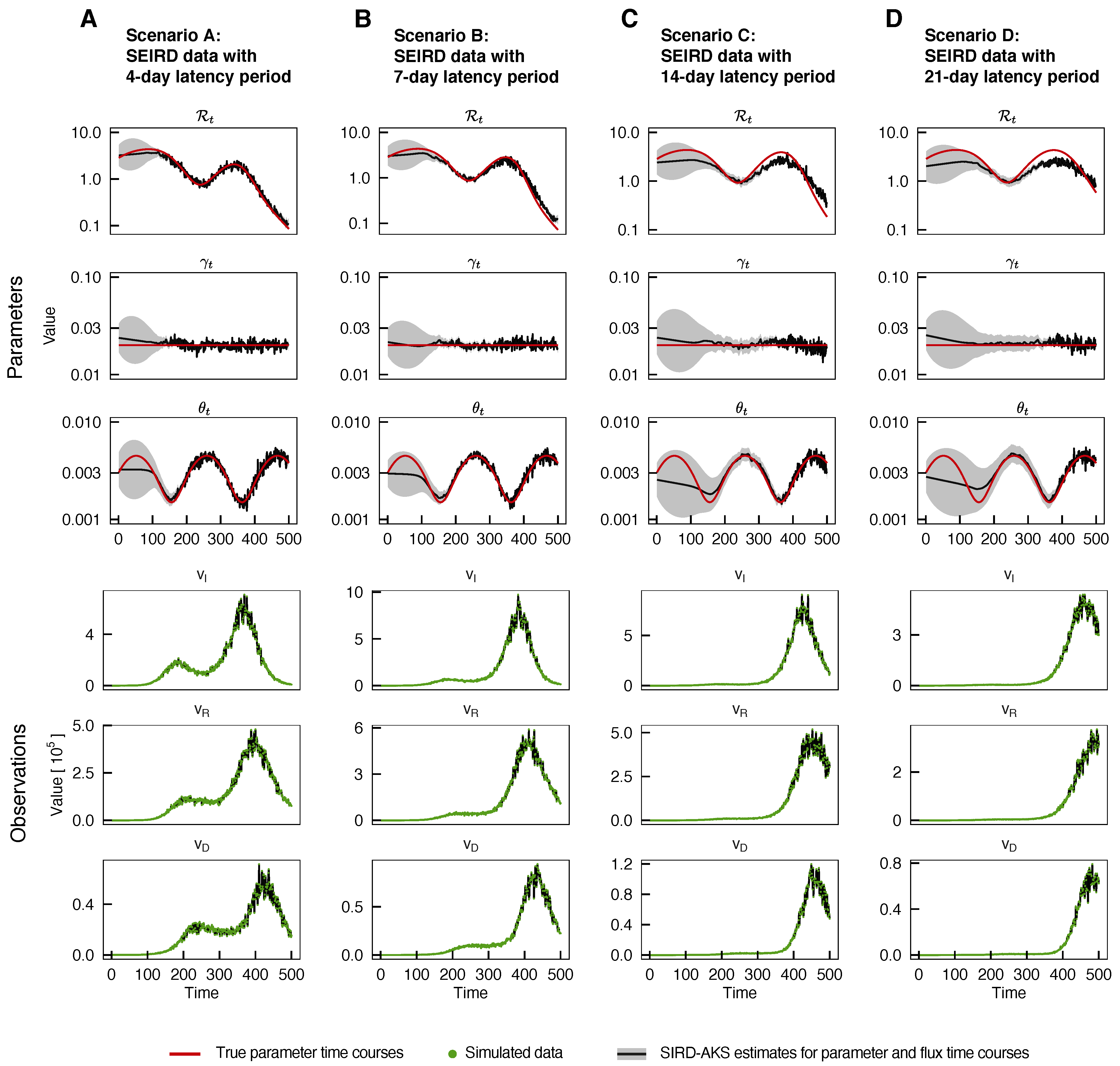
3.3. Influence of Potential Model Misspecifications

Up to this point, we have only shown applications of the SIRD-AKS method to simulated data from the same SIRD model structure. In more realistic applications, however, the true model structure is not known, or as in all real-world scenarios, the chosen model structure is only an appropriate simplification of the real underlying biological process. Therefore, we next investigated the performance of the SIRD-AKS method in light of model misspecifications. To this aim, data were generated from non-SIRD model structures but were analyzed by the AKS method by using the inappropriate SIRD model structure. We tried to reconstruct the time courses of the effective reproduction number in two examples of such intentionally misspecified model structures for the SIRD-AKS method.

First, the so-called SEIRD model was considered for data generation. It constitutes an extension of the SIRD model augmented by a model state of exposed (E) corresponding to individuals that are infected but not yet infectious. This extension is commonly considered when the disease progression underlies an incubation period. The ODE system of the SEIRD model reads

$$\begin{array}{c}\hfill \begin{array}{cc}\hfill \dot{S}& =-\beta ·\frac{S·I}{N_0}\hfill \\ \hfill \dot{E}& =\beta ·\frac{S·I}{N_0}-\delta ·E\hfill \\ \hfill \dot{I}& =\delta ·E-\gamma ·I-\theta ·I\hfill \\ \hfill \dot{R}& =\gamma ·I\hfill \\ \hfill \dot{D}& =\theta ·I,\hfill \end{array}\end{array}$$

(25)

where the reciprocal of the additional parameter ${\delta }^{-1}$ is called the latency period. Note that the limiting case of the SEIRD model for ${\delta }^{-1}\to 0$ is the SIRD model, while for higher values of ${\delta }^{-1}$, the difference between the two models increases and distinct dynamics are expected. To illustrate this transition, four different analyses with latency periods varying from 4 to 21 days were performed.

The SEIRD model Equation (25) was simulated for data generation with time-dependent parameters ${\beta }_t$ and ${\theta }_t$ as well as the time-constant parameter ${\gamma }_t$, following the previous parameter setting I. Again, the true values for the reproduction number ${\mathcal{R}}_t$ were calculated from the model parameters for the SEIRD model [68]. To mimic a realistic application of the presented method in an epidemic scenario, where the true underlying process is not fully known, data from the SEIRD model were analyzed by the SIRD-AKS, and only the daily numbers of the newly infected $v_I$, newly recovered $v_R$ and newly dead $v_D$ were provided as observations to the algorithm. In consequence, the SIRD-AKS is able to estimate the SIRD model states and parameters but cannot infer the transition rate $\delta$ or the exposed state E.

The resulting time courses of the SIRD-AKS estimates are shown in the upper part of Figure 3 with increasing values for the latency period ${\delta }^{-1}$ from panel A to D. Comparing the four simulation scenarios, the different latency periods are reflected both in different dynamics of the observables and in the time courses of the reproduction number ${\mathcal{R}}_t$. As expected, the peak in the observed infections appears later for higher latency periods corresponding to longer times that individuals remain in the exposed state E.

For all scenarios, the SIRD-AKS was applied to the SEIRD data sets, as shown in black in Figure 3A–D. It can be seen that the time courses of the parameters ${\gamma }_t$ and ${\theta }_t$ are throughout accurately obtained. Interestingly, the estimates for the effective reproduction number ${\mathcal{R}}_t$ are also very close to the true values for the low-to-medium latency periods. In contrast, for higher latency periods, the estimates for ${\mathcal{R}}_t$ are slightly shifted to later time points and are also biased towards the characteristic value of ${\mathcal{R}}_t=1$. In total, this shows that the AKS method is able to cope with moderate deviations in the model structure, while more extreme model misspecifications, e.g., latency periods of three weeks, can noticeably influence the result of the estimated time-dependent parameters. Especially, for COVID-19, such a model misspecification does not negatively impact the SIRD-AKS estimation results since a latency period of 5–6 days was typically reported [69].

In order to formulate a model-misspecification problem that is closer to a real-world scenario, we additionally utilized a larger and more complicated model structure that covers a multitude of additional features. For this, we employed the so-called SECIR model that consists of sixteen model states and was developed to obtain a detailed description of the SARS-CoV-2 epidemic in Germany in 2020, including, for example, several infected carrier states as well as diverse hospitalization stages [27]. This model was used for data generation by using parameters values within the allowed parameter ranges as in the original publication. The only deviation is that we replaced the originally estimated time course of the transmission parameter $R_1$ by a simple five-step function. This parameter mainly influences the time course of the true value of the effective reproduction number ${\mathcal{R}}_t$ within the SECIR model, which was calculated according to the respective equation in the original publication and is shown as a reference in red in Figure 4. Within the chosen parameter set for the simulation, the resulting true ${\mathcal{R}}_t$ time course covers a broad range of values, in particular below and above the characteristic value of ${\mathcal{R}}_t=1$. The generated data sets for the newly infected $v_I$, newly recovered $v_R$ and newly dead $v_D$ were again provided as observations of the SIRD-AKS analysis. The estimated time course of the effective reproduction number ${\mathcal{R}}_t$ from the SIRD-AKS with SECIR data is shown as a black line in Figure 4. Except for the level of the first plateau until $t=80$, the ${\mathcal{R}}_t$ value from the SIRD-AKS method shows a similar shape as the true ${\mathcal{R}}_t$ time course and yields almost correct levels on the other plateaus. However, the estimated ${\mathcal{R}}_t$ time course is slightly biased to ${\mathcal{R}}_t=1$ after $t=80$ days.

For a comparison of the different methods, Figure 4 also shows the results for the reproduction number ${\mathcal{R}}_t^{s,\tau }$ calculated by using the incidence-based method from Equation (24) for different values of the fixed serial interval time $s=2,...,10$ days in unit steps and with averaging windows of $\tau =4$ days. It can be clearly seen that the choice of the fixed serial interval time heavily influences the resulting levels of the reproduction number. The Robert Koch Institute (RKI) as the German center for disease control provided officially issued reproduction number values during the SARS-CoV-2 pandemic for Germany based on this method with a chosen fixed serial interval value of $s=4$ days. The accordingly calculated ${\mathcal{R}}_t^{4,4}$ value for the SECIR data set is highlighted in blue in Figure 4. Comparing the blue and red line, it can be concluded that at least for the simulations of the SECIR model and the chosen parameterization, a fixed serial interval of $s=4$ days is not an adequate choice. While the RKI-issued value roughly covers the general form of the time course, it is noticeably biased towards the characteristic value of ${\mathcal{R}}_t=1$. As a consequence, the rate of increase or decay in newly infected individuals within an ongoing disease outbreak would be definitely underestimated.

An appropriate choice of the serial-interval distribution or at least an optimal choice of the fixed serial interval time s would solve this issue, as can be seen from the gray lines in Figure 4. However, it should be noted that the selection of the optimal value for s is difficult in real-world applications and requires additional data or assumptions. That is, the simplicity of the calculation and interpretation by using the incidence-based method comes at the price of required assumptions for the serial interval times.

Some deviations from the true ${\mathcal{R}}_t$ value also appear in the results of the SIRD-AKS method. However, we surmise that these originate from the misspecified model structure. We argue that a clear advantage of the SIRD-AKS method is that it does not rely on additional hyperparameters or distributional assumptions, such as the incidence-based method does on the serial interval time. This renders the SIRD-AKS method to be a de facto non-parametric approach for the estimation of the reproduction number and model parameters in general. As shown in this example, the SIRD-AKS method also yields reasonable results when the internal state-space model does not meet the model structure of the data-generating process. It therefore qualifies for the application to real-world data sets, where the true underlying process is masked and thus the optimal choice of an appropriate fixed serial interval time for the incidence-based method becomes even more difficult.

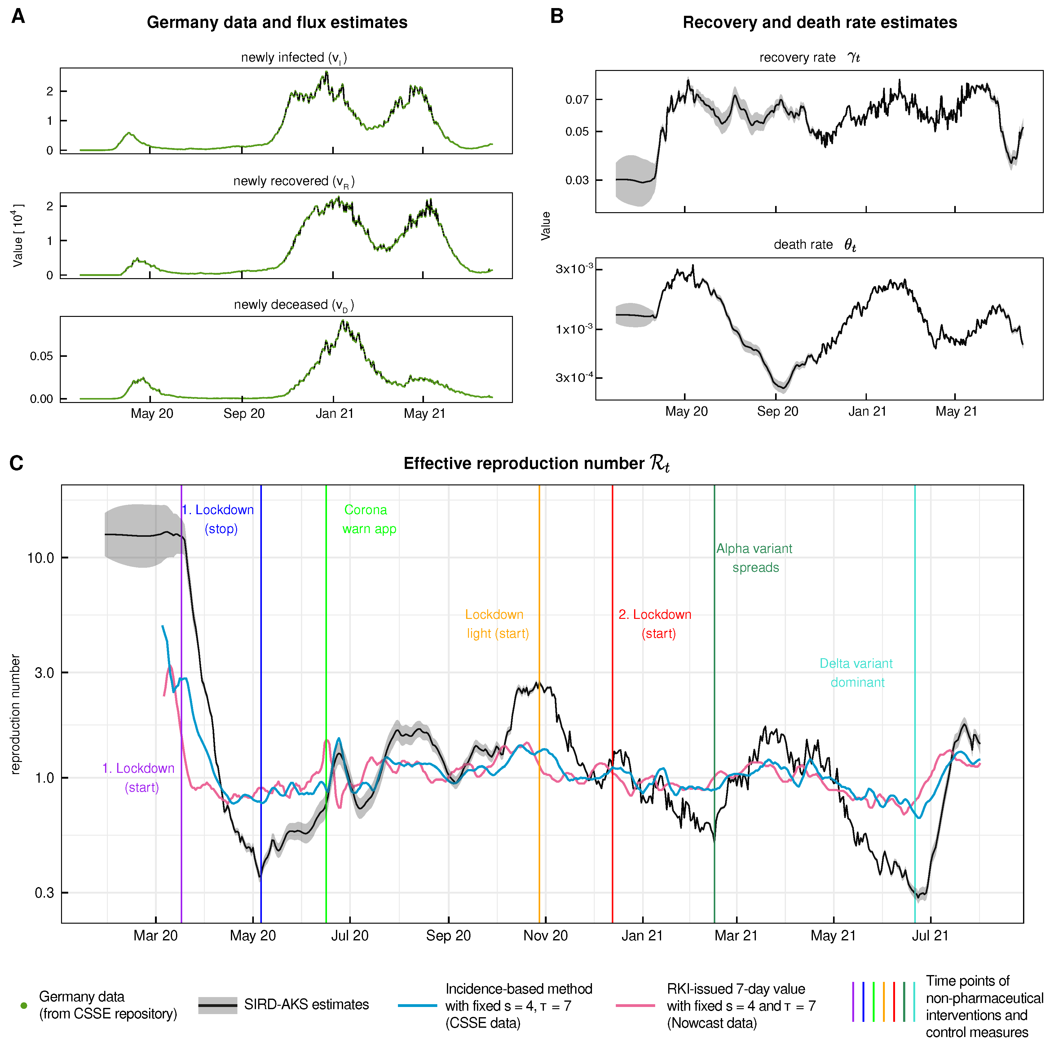
3.4. Application to SARS-CoV-2 Data from Germany

After demonstrating the performance of the SIRD-AKS method for multiple-parameter time courses and model misspecifications in simulated data sets, the method was applied to COVID-19 data from Germany between January 2020 and August 2021. The data were taken from the COVID-19 Data Repository maintained by the Center for Systems Science and Engineering (CSSE) at Johns Hopkins University [70] and is displayed in Figure 5A as green dots. Data pre-processing was performed with a moving average over seven days in order to reduce weekday effects and reporting delays in the raw data.

Figure 5A shows the analyzed data and estimated time courses of the observed fluxes for the newly infected $v_I$, newly recovered $v_R$ and newly dead $v_D$. The estimated time courses for the recovery rate ${\gamma }_t$ and death rate ${\theta }_t$ are shown in Figure 5B. The fluctuations in the death rate are in line with the time periods when more old people had been reported as being infected, i.e., from April to June and from November to February 2020 [71]. This also agrees with previous studies showing that the mortality of COVID-19 is heavily linked to the patient’s age [72,73].

The estimated time-dependent reproduction rate ${\mathcal{R}}_t$ from the SIRD-AKS method is shown as a black line in Figure 5C. For comparison, two additional ${\mathcal{R}}_t$ values are provided, which are both based on the previously discussed incidence-based method and assume a fixed serial interval of $s=4$ days and an averaging window of $\tau =7$ days. However, they use different data sources. The ${\mathcal{R}}_t$ value shown as a blue line is calculated from the same data from [70] that were also analyzed by using the SIRD-AKS method. The other shown value in magenta is the officially issued and so-called seven-day${\mathcal{R}}_t^{4,7}$ value from the RKI [66]. The difference is that it does not use the raw data from the CSSE repository but instead applies an additional so-called Nowcasting pre-processing method that copes with the redistribution of the case numbers for the elimination of reporting delays [74]. Both incidence-based methods show a similar time course for ${\mathcal{R}}_t$ but with peaks that seem to be shifted by a couple of days, presumably because of the case-number redistribution.

Figure 5. Application of the SIRD-AKS to SARS-CoV-2 data of Germany from the CSSE repository. (A): Incidence data taken from [70] for March 2020 until August 2021 are shown in green. SIRD-AKS results for the fluxes of newly infected, newly recovered and newly deceased is shown as black line. (B): After an initial rise, the SIRD-AKS estimated for the recovery rate ${\gamma }_t$ stays nearly constant, while the estimated death rate ${\theta }_t$ shows a dynamic with two peaks at around May–June 2020 and February–March 2021. These time points coincide with periods of high hospitalization states and where mostly older people were infected [71]. (C): The SIRD-AKS estimates (black) for the reproduction number are displayed in comparison to the seven-day reproduction number based on Nowcasting data and published by the RKI in magenta [66] as well as the calculated ${\mathcal{R}}_t^{s,\tau }$ incidence-based method in blue that is based on CSSE data. Both incidence-based methods assume a fixed serial time of $s=4$ days and averaging window of $\tau =7$ days. Time points of essential control measures are indicated by colored vertical lines [75].

Figure 5. Application of the SIRD-AKS to SARS-CoV-2 data of Germany from the CSSE repository. (A): Incidence data taken from [70] for March 2020 until August 2021 are shown in green. SIRD-AKS results for the fluxes of newly infected, newly recovered and newly deceased is shown as black line. (B): After an initial rise, the SIRD-AKS estimated for the recovery rate ${\gamma }_t$ stays nearly constant, while the estimated death rate ${\theta }_t$ shows a dynamic with two peaks at around May–June 2020 and February–March 2021. These time points coincide with periods of high hospitalization states and where mostly older people were infected [71]. (C): The SIRD-AKS estimates (black) for the reproduction number are displayed in comparison to the seven-day reproduction number based on Nowcasting data and published by the RKI in magenta [66] as well as the calculated ${\mathcal{R}}_t^{s,\tau }$ incidence-based method in blue that is based on CSSE data. Both incidence-based methods assume a fixed serial time of $s=4$ days and averaging window of $\tau =7$ days. Time points of essential control measures are indicated by colored vertical lines [75].

When compared to the estimate from the SIRD-AKS method, both incidence-based values again lie closer to ${\mathcal{R}}_t=1$. The time course from the SIRD-AKS shows a larger variety of peak heights in both directions and more deviations from ${\mathcal{R}}_t=1$ on longer time scales. This becomes even more prominent when the changes in the reproduction numbers are compared to the time points of new non-pharmaceutical interventions and control measures, as indicated by vertical lines. While the incidence-based ${\mathcal{R}}_t$ values likewise decrease drastically at the start of the first nation-wide lockdown in March 2020, the end of the first lockdown is only visible as a trend change in the SIRD-AKS reproduction number, but not in the incidence-based approaches. A similar case occurs for the so-called lockdown light in November 2020 and second nation-wide lockdown in December 2020 [75]. Both incidence-based measures barely show any effect on the reproduction number, while the SIRD-AKS estimate shows a fluctuating yet undoubtedly decreasing trend until the approximate time point where the SARS-CoV-2 Alpha variant spread in Germany.

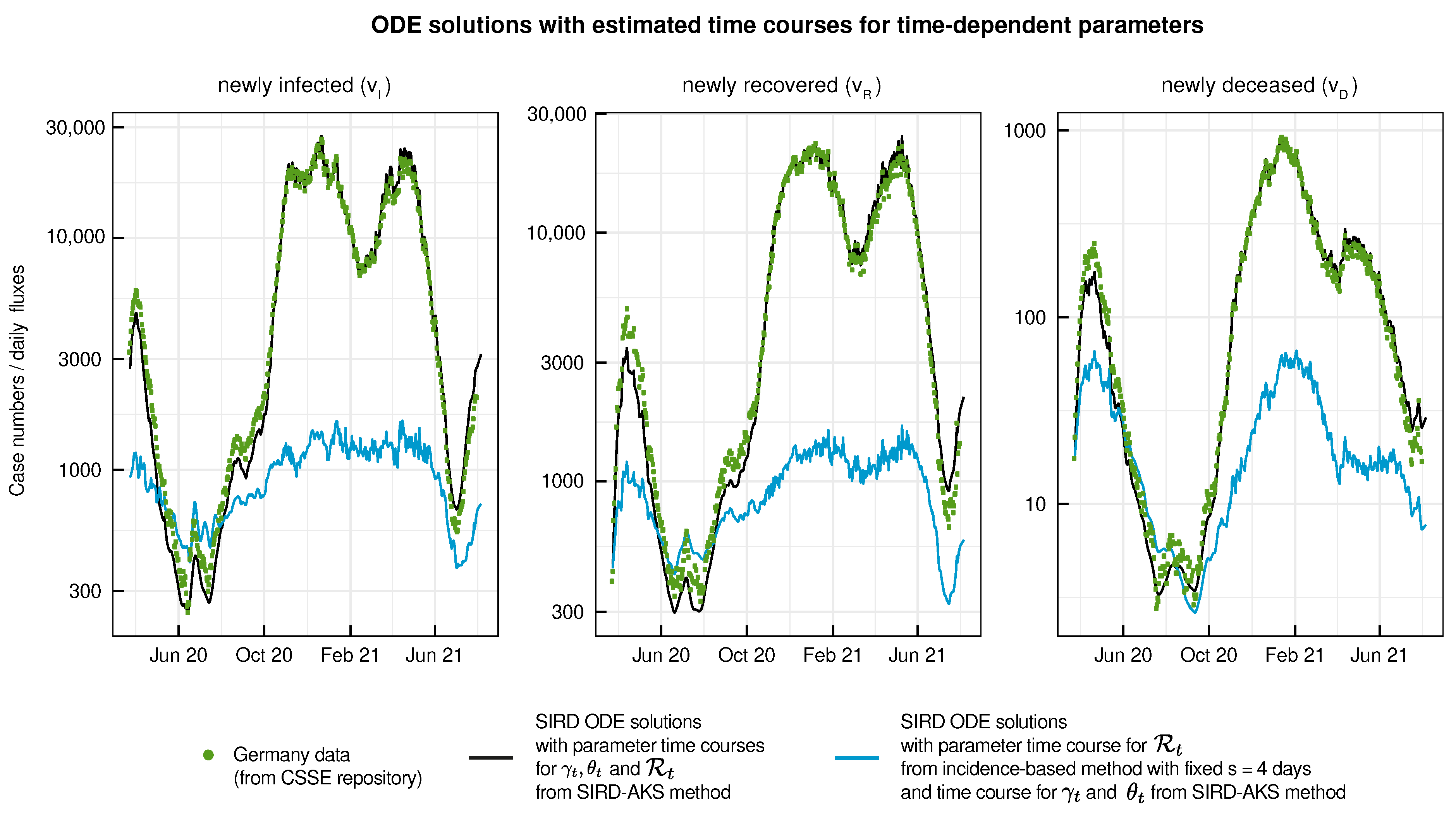
3.5. Validation of Parameter Time-Course Estimates in an ODE Model

The presented SIRD-AKS method is based on the transition of the model structure from the time-continuous ODE system to the time-discrete and recursive formulation in the state space. Further, estimates for the time-dependent parameters are in fact augmented states in the state space, interpreted as parameter time courses. We asked whether these parameter time courses produce coherent dynamics when being incorporated into the corresponding ODE system as input functions.

To perform this consistency check, we plugged in the estimated time courses for the parameters ${\mathcal{R}}_t,{\gamma }_t$ and ${\theta }_t$ from Figure 5B,C into the ODEs of the reparameterized SIRD model in Equation (21). To choose appropriate initial values for the numerical solution of this ODE system, the values of the SIRD-AKS estimates at time point $k=62$, i.e., 24 March 2020, were chosen. This time point corresponds to the first time point where the estimated uncertainties of the time-dependent parameters become adequately small. It also coincides with the starting point of the large initial decrease in the time course of ${\mathcal{R}}_t$, c.f. Figure 5C. The results of the numerical simulation of the time-continuous ODE system with time-dependent parameters are shown in Figure 6 as a black line. It is remarkable that all three trajectories are very well in agreement with the flux data for $v_I$, $v_R$ and $v_D$ that went into the previous AKS analysis, shown as green dots in Figure 6.

This confirms that the parameter time courses estimated from the incidence data by the AKS method are indeed able to reassemble the correct dynamics in the ODE solutions. The presented AKS method thus qualifies as a potential input-estimation approach for ODE models in general.

For comparison, the same ODE simulation was performed by utilizing the alternative ${\mathcal{R}}_t$ time course calculated from the incidence-based method with a fixed serial-interval time of $s=4$ days and an averaging interval of $\tau =7$ days, as presented above in Figure 5C as a blue line. Since this methods lacks estimates for parameters ${\gamma }_t$ and ${\theta }_t$ as required to solve the ODE system, time-course estimates for ${\gamma }_t$ and ${\theta }_t$ from the SIRD-AKS method were chosen. The resulting incidence-based ODE trajectories are displayed as blue lines in Figure 6.

In contrast to the ODE trajectories with SIRD-AKS estimates, the ODE solutions with incidence-based ${\mathcal{R}}_t$ do not agree well with the data. Although the overall dynamic activity of the data is approximately covered, it does not capture certain details of the data series well, e.g., the partial drop in the infected flux during the second wave in February 2021. Furthermore, the predicted amplitudes of newly infected individuals are not adequately met and thus the overall pandemic situation would be underestimated.

It should be noted that the lack of estimates for ${\gamma }_t$ and ${\theta }_t$ from the incidence-based method renders some difficulty for a fair method comparison within this ODE-validation approach.

In conclusion, the incidence-based method does not provide an estimate for the reproduction number ${\mathcal{R}}_t$ that can be used as an input function in the addressed ODE model. Instead, for the shown real-word application, the incidence-based method ${\mathcal{R}}_t$ generates an ODE solution that differs from the observations in orders of magnitude. In contrast, the SIRD-AKS method reassembles an adequate ODE solution, even in the potentially over-simplified SIRD model.

4. Discussion

The general task of estimating time-dependent parameters in ODE models, also referred to as input-function estimation, is known to be conceptually difficult. Either a particular function class, i.e., a parameterization of a general input function, needs to be provided, or the initial value problem of solving the ODE needs to be transferred into a boundary value problem for which no good optimizers are available [36].

To remedy this, we present in this work a non-parametric model-based estimation for all time-dependent parameters in epidemiological ODE models by combining an Expectation-Maximization algorithm with the Augmented Kalman Smoother (AKS) algorithm.

The approach is able to estimate the time dependencies in multiple model parameters and independently from the particular input function class. While other approaches exist that also take advantage of Kalman filter methods for the estimation of a single time dependency in compartmental models [76], this approach is more general and enables the estimation of all time-dependent model parameters simultaneously.

We showed the performance of our AKS method by using an SIRD core model structure (SIRD-AKS) in diverse simulation settings. The SIRD-AKS performs well even with high noise levels and under different degrees of model misspecification. Thus, the method also yields meaningful estimates in situations where the details of the data-generating process remain unknown, meaning that the assumed AKS model structure does not perfectly cover the true process structure. In particular, the presented approach only utilizes incidence data of infected, recovered and deceased individuals and, as a major advantage compared to existing methods [27,66], does not require any further prior knowledge on the analyzed disease.

When applying the SIRD-AKS method to COVID-19 data from Germany, it can be observed that all the parameter time-course estimates are plausible, and in particular, the effective reproduction number ${\mathcal{R}}_t$ estimate displays the impact of all relevant non-pharmaceutical interventions and applied control measures during the SARS-CoV-2 pandemic in Germany. Further, the simultaneously estimated death rate ${\theta }_t$ matches well with the time pattern of how many elderly people were infected by the disease.

We further compared our SIRD-AKS method to an alternative approach for the estimation of ${\mathcal{R}}_t$, which considerably depends on the choice for the value of the assumed Dirac $\delta$-distributed serial interval.

In contrast, the SIRD-AKS method is independent of the distribution of the serial interval, and therefore, it does not require any information on the assumed serial interval time as a hyperparameter. Instead, our approach internally copes with the serial interval through the ODE model and is not affected by any inadequate assumptions on the serial-interval distribution. Even if the serial-interval distribution is also subject to change over time, as, for example, reported in [77], this is compensated by the general time dependency e.g., of the transmission parameter ${\beta }_t$ in the SIRD model.

Compared to the incidence-based method, the SIRD-AKS estimate for the effective reproduction number ${\mathcal{R}}_t$ shows the pandemic situation more clearly as it is less biased towards ${\mathcal{R}}_t=1$. Furthermore, we checked the appropriateness of the estimated parameter time courses obtained by using the SIRD-AKS method by plugging them back into the original ODE model. While the incidence-based estimates yielded case numbers that were orders of magnitude below the original data, we were able to correctly reassemble the case numbers by the ODE model from the SIRD-AKS estimates.

5. Conclusions

In summary, the SIRD-AKS method is a non-parametric model-based estimation approach for the reproduction number and other time-dependent model parameters that only requires incidence data of newly infected, recovered and deceased individuals. If one would want to analyze different epidemiological data sets independently of COVID-19 or any other diseases with a short-enough incubation time (${\delta }^{-1}<14d$, see Section 3.3), the method would only need to be provided the respective data sets, and no changes to the method would be required. Since the presented approach is not restricted to epidemiological ODE models by construction, it might also be used for input-function estimation in non-linear ODE models in general.

References

1. Jones, K.E.; Patel, N.G.; Levy, M.A.; Storeygard, A.; Balk, D.; Gittleman, J.L.; Daszak, P. Global trends in emerging infectious diseases. Nature 2008, 451, 990–993. [Google Scholar] [CrossRef]
2. World Health Organization. Vector-Borne Diseases; Technical Report; WHO Regional Office for South-East Asia: New Delhi, India, 2014. [Google Scholar]
3. Hethcote, H.W. The mathematics of infectious diseases. SIAM Rev. 2000, 42, 599–653. [Google Scholar] [CrossRef]
4. Murray, J.D. Mathematical Biology: I. An Introduction. Interdisciplinary Applied Mathematics; Springer: Berlin/Heidelberg, Germany, 2002. [Google Scholar]
5. Brauer, F.; Castillo-Chavez, C.; Castillo-Chavez, C. Mathematical Models in Population Biology and Epidemiology; Springer: Berlin/Heidelberg, Germany, 2012; Volume 2. [Google Scholar]
6. Tönsing, C.; Timmer, J.; Kreutz, C. Profile likelihood-based analyses of infectious disease models. Stat. Methods Med. Res. 2018, 27, 1979–1998. [Google Scholar] [CrossRef]
7. Abboubakar, H.; Guidzavaï, A.K.; Yangla, J.; Damakoa, I.; Mouangue, R. Mathematical modeling and projections of a vector-borne disease with optimal control strategies: A case study of the Chikungunya in Chad. Chaos Solitons Fractals 2021, 150, 111197. [Google Scholar] [CrossRef]
8. Barbarossa, M.V.; Fuhrmann, J.; Meinke, J.H.; Krieg, S.; Varma, H.V.; Castelletti, N.; Lippert, T. Modeling the spread of COVID-19 in Germany: Early assessment and possible scenarios. PLoS ONE 2020, 15, e0238559. [Google Scholar] [CrossRef]
9. Dehning, J.; Zierenberg, J.; Spitzner, F.P.; Wibral, M.; Neto, J.P.; Wilczek, M.; Priesemann, V. Inferring change points in the spread of COVID-19 reveals the effectiveness of interventions. Science 2020, 369, eabb9789. [Google Scholar] [CrossRef]
10. Bai, Z.; Gong, Y.; Tian, X.; Cao, Y.; Liu, W.; Li, J. The rapid assessment and early warning models for COVID-19. Virol. Sin. 2020, 35, 272–279. [Google Scholar] [CrossRef]
11. Ferguson, N.; Laydon, D.; Nedjati Gilani, G.; Imai, N.; Ainslie, K.; Baguelin, M.; Bhatia, S.; Boonyasiri, A.; Cucunuba Perez, Z.; Cuomo-Dannenburg, G.; et al. Report 9: Impact of Non-Pharmaceutical Interventions (NPIs) to Reduce COVID-19 Mortality and Healthcare Demand; Imperial College London: London, UK, 2020. [Google Scholar]
12. Jarvis, C.I.; Van Zandvoort, K.; Gimma, A.; Prem, K.; Klepac, P.; Rubin, G.J.; Edmunds, W.J. Quantifying the impact of physical distance measures on the transmission of COVID-19 in the UK. BMC Med. 2020, 18, 1–10. [Google Scholar] [CrossRef]
13. Latsuzbaia, A.; Herold, M.; Bertemes, J.P.; Mossong, J. Evolving social contact patterns during the COVID-19 crisis in Luxembourg. PLoS ONE 2020, 15, e0237128. [Google Scholar] [CrossRef]
14. Ivorra, B.; Ferrández, M.R.; Vela-Pérez, M.; Ramos, A.M. Mathematical modeling of the spread of the coronavirus disease 2019 (COVID-19) taking into account the undetected infections. The case of China. Commun. Nonlinear Sci. Numer. Simul. 2020, 88, 105303. [Google Scholar] [CrossRef]
15. Contento, L.; Castelletti, N.; Raimundez, E.; Le Gleut, R.; Schaelte, Y.; Stapor, P.; Hinske, L.C.; Hoelscher, M.; Wieser, A.; Radon, K.; et al. Integrative modelling of reported case numbers and seroprevalence reveals time-dependent test efficiency and infection rates. medRxiv 2021. [Google Scholar]
16. Rockett, R.J.; Arnott, A.; Lam, C.; Sadsad, R.; Timms, V.; Gray, K.A.; Eden, J.S.; Chang, S.; Gall, M.; Draper, J.; et al. Revealing COVID-19 transmission in Australia by SARS-CoV-2 genome sequencing and agent-based modeling. Nat. Med. 2020, 26, 1398–1404. [Google Scholar] [CrossRef]
17. Truszkowska, A.; Behring, B.; Hasanyan, J.; Zino, L.; Butail, S.; Caroppo, E.; Jiang, Z.P.; Rizzo, A.; Porfiri, M. High-resolution agent-based modeling of COVID-19 spreading in a small town. Adv. Theory Simul. 2021, 4, 2000277. [Google Scholar] [CrossRef]
18. Hoertel, N.; Blachier, M.; Blanco, C.; Olfson, M.; Massetti, M.; Rico, M.S.; Limosin, F.; Leleu, H. A stochastic agent-based model of the SARS-CoV-2 epidemic in France. Nat. Med. 2020, 26, 1417–1421. [Google Scholar] [CrossRef]
19. Capaldi, A.; Behrend, S.; Berman, B.; Smith, J.; Wright, J.; Lloyd, A.L. Parameter estimation and uncertainty quantication for an epidemic model. Math. Biosci. Eng. 2012, 9, 553. [Google Scholar]
20. Kermack, W.O.; McKendrick, A.G. Contributions to the mathematical theory of epidemics–I. 1927. Bull. Math. Biol. 1991, 53, 33–55. [Google Scholar]
21. Chen, X.; Li, J.; Xiao, C.; Yang, P. Numerical solution and parameter estimation for uncertain SIR model with application to COVID-19. Fuzzy Optim. Decis. Mak. 2021, 20, 189–208. [Google Scholar] [CrossRef]
22. Bani-Yaghoub, M.; Gautam, R.; Shuai, Z.; Van Den Driessche, P.; Ivanek, R. Reproduction numbers for infections with free-living pathogens growing in the environment. J. Biol. Dyn. 2012, 6, 923–940. [Google Scholar] [CrossRef]
23. Wieland, F.G.; Hauber, A.L.; Rosenblatt, M.; Tönsing, C.; Timmer, J. On structural and practical identifiability. Curr. Opin. Syst. Biol. 2021, 25, 60–69. [Google Scholar] [CrossRef]
24. Massonis, G.; Banga, J.R.; Villaverde, A.F. Structural identifiability and observability of compartmental models of the COVID-19 pandemic. Annu. Rev. Control. 2020, 51, 441–459. [Google Scholar] [CrossRef]
25. Godio, A.; Pace, F.; Vergnano, A. SEIR modeling of the Italian epidemic of SARS-CoV-2 using computational swarm intelligence. Int. J. Environ. Res. Public Health 2020, 17, 3535. [Google Scholar] [CrossRef]
26. Raimúndez, E.; Dudkin, E.; Vanhoefer, J.; Alamoudi, E.; Merkt, S.; Fuhrmann, L.; Bai, F.; Hasenauer, J. COVID-19 outbreak in Wuhan demonstrates the limitations of publicly available case numbers for epidemiological modeling. Epidemics 2021, 34, 100439. [Google Scholar] [CrossRef]
27. Khailaie, S.; Mitra, T.; Bandyopadhyay, A.; Schips, M.; Mascheroni, P.; Vanella, P.; Lange, B.; Binder, S.C.; Meyer-Hermann, M. Development of the reproduction number from coronavirus SARS-CoV-2 case data in Germany and implications for political measures. BMC Med. 2021, 19, 1–16. [Google Scholar] [CrossRef]
28. Rahmandad, H.; Lim, T.Y.; Sterman, J. Behavioral dynamics of COVID-19: Estimating under-reporting, multiple waves, and adherence fatigue across 92 nations. Syst. Dyn. Rev. 2021, 37, 5–31. [Google Scholar] [CrossRef]
29. Prodanov, D. Analytical parameter estimation of the SIR epidemic model. Applications to the COVID-19 pandemic. Entropy 2021, 23, 59. [Google Scholar] [CrossRef]
30. Jo, H.; Son, H.; Hwang, H.J.; Jung, S.Y. Analysis of COVID-19 spread in South Korea using the SIR model with time-dependent parameters and deep learning. medRxiv 2020. [Google Scholar]
31. Hong, H.G.; Li, Y. Estimation of time-varying reproduction numbers underlying epidemiological processes: A new statistical tool for the COVID-19 pandemic. PLoS ONE 2020, 15, e0236464. [Google Scholar] [CrossRef]
32. Kolokolnikov, T.; Iron, D. Law of mass action and saturation in SIR model with application to coronavirus modelling. Infect. Dis. Model. 2021, 6, 91–97. [Google Scholar] [CrossRef]
33. Capistrán, M.A.; Moreles, M.A.; Lara, B. Parameter estimation of some epidemic models. The case of recurrent epidemics caused by respiratory syncytial virus. Bull. Math. Biol. 2009, 71, 1890–1901. [Google Scholar] [CrossRef]
34. Merow, C.; Urban, M.C. Seasonality and uncertainty in global COVID-19 growth rates. Proc. Natl. Acad. Sci. USA 2020, 117, 27456–27464. [Google Scholar] [CrossRef]
35. Refisch, L.; Lorenz, F.; Riedlinger, T.; Taubenböck, H.; Fischer, M.; Grabenhenrich, L.; Wolkewitz, M.; Binder, H.; Kreutz, C. Data-driven prediction of COVID-19 cases in Germany for decision making. BMC Med. Res. Methodol. 2022, 22, 1–13. [Google Scholar] [CrossRef]
36. Kaschek, D.; Timmer, J. A variational approach to parameter estimation in ordinary differential equations. BMC Syst. Biol. 2012, 6, 1–8. [Google Scholar] [CrossRef]
37. Engelhardt, B.; Frőhlich, H.; Kschischo, M. Learning (from) the errors of a systems biology model. Sci. Rep. 2016, 6, 20772. [Google Scholar] [CrossRef]
38. Villaverde, A.F.; Tsiantis, N.; Banga, J.R. Full observability and estimation of unknown inputs, states and parameters of nonlinear biological models. J. R. Soc. Interface 2019, 16, 20190043. [Google Scholar] [CrossRef]
39. Kreutz, C. A new approximation approach for transient differential equation models. Front. Phys. 2020, 8, 70. [Google Scholar] [CrossRef]
40. Camacho, A.; Cazelles, B. Does homologous reinfection drive multiple-wave influenza outbreaks? Accounting for immunodynamics in epidemiological models. Epidemics 2013, 5, 187–196. [Google Scholar] [CrossRef]
41. Camacho, A.; Kucharski, A.; Funk, S.; Breman, J.; Piot, P.; Edmunds, W. Potential for large outbreaks of Ebola virus disease. Epidemics 2014, 9, 70–78. [Google Scholar] [CrossRef]
42. Dureau, J.; Kalogeropoulos, K.; Vickerman, P.; Pickles, M.; Boily, M.C. A Bayesian approach to estimate changes in condum use from limited human immunodeficiency virus prevalence data. J. R. Stat. Soc. Ser. C 2016, 65, 237–257. [Google Scholar] [CrossRef]
43. Yang, W.; Karspeck, A.; Shaman, J. Comparison of Filtering Methods for the Modeling and Retrospective Forecasting of Influenza Epidemics. PLoS Comput. Biol. 2014, 10, 1–15. [Google Scholar] [CrossRef]
44. Cazelles, B.; Champagne, C.; Nguyen-Van-Yen, B.; Comiskey, C.; Vergu, E.; Roche, B. A mechanistic and data-driven reconstruction of the time-varying reproduction number: Application to the COVID-19 epidemic. PLoS Comput. Biol. 2021, 17, 1–20. [Google Scholar] [CrossRef]
45. Dureau, J.; Kalogeropoulos, K.; Baguelin, M. Capturing the time-varying drivers of an epidemic using stochastic dynamical systems. Biostatistics 2013, 14, 541–555. [Google Scholar] [CrossRef]
46. Endo, A.; van Leeuwen, E.; Baguelin, M. Introduction to particle Markov-chain Monte Carlo for disease dynamics modellers. Epidemics 2019, 29, 100363. [Google Scholar] [CrossRef]
47. Raanes, P.N. On the ensemble Rauch-Tung-Striebel smoother and its equivalence to the ensemble Kalman smoother. Q. J. R. Meteorol. Soc. 2016, 142, 1259–1264. [Google Scholar] [CrossRef]
48. Hasan, A.; Susanto, H.; Tjahjono, V.; Kusdiantara, R.; Putri, E.; Nuraini, N.; Hadisoemarto, P. A new estimation method for COVID-19 time-varying reproduction number using active cases. Sci. Rep. 2022, 12, 6675. [Google Scholar] [CrossRef]
49. Shumway, R.H.; Stoffer, D.S. An approach to time series smoothing and forecasting using the em algorithm. J. Time Ser. Anal. 1982, 3, 253–264. [Google Scholar] [CrossRef]
50. Pulido, M.; Tandeo, P.; Bocquet, M.; Carrassi, A.; Lucini, M. Stochastic parameterization identification using ensemble Kalman filtering combined with maximum likelihood methods. Tellus A Dyn. Meteorol. Oceanogr. 2018, 70, 1442099. [Google Scholar] [CrossRef]
51. Hermes, J.; Rosenblatt, M.; Tönsing, C.; Timmer, J. Non-parametric model-based estimation of the effective reproduction number for SARS-CoV-2. AIP Conf. Proc. 2023, 2872, 030006. [Google Scholar] [CrossRef]
52. Keeling, M.J.; Rohani, P. Modeling Infectious Diseases in Humans and Animals; Princeton University Press: Princeton, NJ, USA, 2011. [Google Scholar]
53. Nishiura, H.; Chowell, G. The effective reproduction number as a prelude to statistical estimation of time-dependent epidemic trends. In Mathematical and Statistical Estimation Approaches in Epidemiology; Springer: Berlin/Heidelberg, Germany, 2009; pp. 103–121. [Google Scholar]
54. Raue, A.; Schilling, M.; Bachmann, J.; Matteson, A.; Schelke, M.; Kaschek, D.; Hug, S.; Kreutz, C.; Harms, B.D.; Theis, F.J.; et al. Lessons learned from quantitative dynamical modeling in systems biology. PLoS ONE 2013, 8, e74335. [Google Scholar] [CrossRef]
55. Raue, A.; Steiert, B.; Schelker, M.; Kreutz, C.; Maiwald, T.; Hass, H.; Vanlier, J.; Tönsing, C.; Adlung, L.; Engesser, R.; et al. Data2Dynamics: A modeling environment tailored to parameter estimation in dynamical systems. Bioinformatics 2015, 31, 3558–3560. [Google Scholar] [CrossRef]
56. Stapor, P.; Weindl, D.; Ballnus, B.; Hug, S.; Loos, C.; Fiedler, A.; Krause, S.; Hroß, S.; Fröhlich, F.; Hasenauer, J. PESTO: Parameter estimation toolbox. Bioinformatics 2018, 34, 705–707. [Google Scholar] [CrossRef]
57. Loos, C.; Krause, S.; Hasenauer, J. Hierarchical optimization for the efficient parametrization of ODE models. Bioinformatics 2018, 34, 4266–4273. [Google Scholar] [CrossRef]
58. Kaschek, D.; Mader, W.; Fehling-Kaschek, M.; Rosenblatt, M.; Timmer, J. Dynamic modeling, parameter estimation, and uncertainty analysis in R. J. Stat. Softw. 2019, 88, 1–32. [Google Scholar] [CrossRef]
59. Schelker, M.; Raue, A.; Timmer, J.; Kreutz, C. Comprehensive estimation of input signals and dynamics in biochemical reaction networks. Bioinformatics 2012, 28, i529–i534. [Google Scholar] [CrossRef]
60. Kalman, R.E. A new approach to linear filtering and prediction problems. J. Basic Eng. 1960, 82, 35–45. [Google Scholar] [CrossRef]
61. Carrassi, A.; Vannitsem, S. State and parameter estimation with the extended Kalman filter: An alternative formulation of the model error dynamics. Q. J. R. Meteorol. Soc. 2011, 137, 435–451. [Google Scholar] [CrossRef]
62. Sun, X.; Jin, L.; Xiong, M. Extended Kalman filter for estimation of parameters in nonlinear state-space models of biochemical networks. PLoS ONE 2008, 3, e3758. [Google Scholar] [CrossRef]
63. Rauch, H.E.; Tung, F.; Striebel, C.T. Maximum likelihood estimates of linear dynamic systems. AIAA J. 1965, 3, 1445–1450. [Google Scholar] [CrossRef]
64. Dreano, D.; Tandeo, P.; Pulido, M.; Ait-El-Fquih, B.; Chonavel, T.; Hoteit, I. Estimating model-error covariances in nonlinear state-space models using Kalman smoothing and the Expectation-Maximization algorithm. Q. J. R. Meteorol. Soc. 2017, 143, 1877–1885. [Google Scholar] [CrossRef]
65. Cori, A.; Ferguson, N.M.; Fraser, C.; Cauchemez, S. A new framework and software to estimate time-varying reproduction numbers during epidemics. Am. J. Epidemiol. 2013, 178, 1505–1512. [Google Scholar] [CrossRef]
66. der Heiden, M.; Hamouda, O. Schätzung der Aktuellen Entwicklung der SARS-CoV-2-Epidemie in Deutschland–Nowcasting. 2020. Available online: https://edoc.rki.de/handle/176904/6650.4 (accessed on 12 November 2021).
67. Soetaert, K.; Petzoldt, T.; Setzer, R.W. Solving differential equations in R: Package deSolve. J. Stat. Softw. 2010, 33, 1–25. [Google Scholar] [CrossRef]
68. Van den Driessche, P. Reproduction numbers of infectious disease models. Infect. Dis. Model. 2017, 2, 288–303. [Google Scholar] [CrossRef]
69. Xin, H.; Li, Y.; Wu, P.; Li, Z.; Lau, E.H.Y.; Qin, Y.; Wang, L.; Cowling, B.J.; Tsang, T.K.; Li, Z. Estimating the Latent Period of Coronavirus Disease 2019 (COVID-19). Clin. Infect. Dis. 2021, 74, 1678–1681. [Google Scholar] [CrossRef]
70. Dong, E.; Du, H.; Gardner, L. An interactive web-based dashboard to track COVID-19 in real time. Lancet Infect. Dis. 2020, 20, 533–534. [Google Scholar] [CrossRef]
71. Staerk, C.; Wistuba, T.; Mayr, A. Estimating effective infection fatality rates during the course of the COVID-19 pandemic in Germany. BMC Public Health 2021, 21, 1073. [Google Scholar] [CrossRef]
72. Yanez, N.D.; Weiss, N.S.; Romand, J.A.; Treggiari, M.M. COVID-19 mortality risk for older men and women. BMC Public Health 2020, 20, 1742. [Google Scholar] [CrossRef]
73. Ho, F.K.; Petermann-Rocha, F.; Gray, S.R.; Jani, B.D.; Katikireddi, S.V.; Niedzwiedz, C.L.; Foster, H.; Hastie, C.E.; Mackay, D.F.; Gill, J.M.; et al. Is older age associated with COVID-19 mortality in the absence of other risk factors? General population cohort study of 470,034 participants. PLoS ONE 2020, 15, e0241824. [Google Scholar] [CrossRef]
74. Höhle, M.; an der Heiden, M. Bayesian nowcasting during the STEC O104: H4 outbreak in Germany, 2011. Biometrics 2014, 70, 993–1002. [Google Scholar] [CrossRef]
75. Fazit Communication GmbH. The Federal Government Informs about the Corona Crisis. 2021. Available online: https://www.deutschland.de/en/news/german-federal-government-informs-about-the-corona-crisis (accessed on 22 October 2021).
76. Arroyo-Marioli, F.; Bullano, F.; Kucinskas, S.; Rondón-Moreno, C. Tracking R of COVID-19: A new real-time estimation using the Kalman filter. PLoS ONE 2021, 16, e0244474. [Google Scholar] [CrossRef]
77. Ali, S.T.; Wang, L.; Lau, E.H.; Xu, X.K.; Du, Z.; Wu, Y.; Leung, G.M.; Cowling, B.J. Serial interval of SARS-CoV-2 was shortened over time by nonpharmaceutical interventions. Science 2020, 369, 1106–1109. [Google Scholar] [CrossRef]
Figure 1. Estimation of multiple time-dependent parameters. (A): The classical SIRD model was simulated with a time-constant parameter γ and time-dependent parameters β t and θ t . From these parameters, the effective reproduction number R t was calculated via Equation (3). True parameter time courses and states are depicted as red solid lines and red dashed lines, respectively. Therefore, data were simulated at 375 equidistant time points for the observed fluxes v D , v I and v R , as indicated by green dots. The SIRD-AKS is based on the reparameterized SIRD model and thus does not yield estimates for β t or S but instead directly for R t . The estimates of the SIRD-AKS are shown as black solid lines with gray bands for their uncertainties. Results are shown on logarithmic scale. The results of the the SIRD-AKS algorithm are able to describe the data and are in good agreement with the true parameter time courses, both for the time-constant and time-dependent parameters. Note that the SIRD-AKS estimates for the states overlap with the true time courses of the model states. (B,C): In different parameter settings, simulation was performed with time-constant parameters γ and θ , whereas β t was either chosen as a stochastic process (B) or as a step function (C), respectively. The corresponding values for R t were computed by using Equation (3). In both cases, the SIRD-AKS results retrieve the true parameter time courses adequately.
Algorithms 16 00533 g001
Figure 2. Performance of SIRD-AKS is robust towards high noise levels in the data. (AD): The SIRD model was simulated with a time-varying β t and time-constant γ t and θ t , as shown in red. The parameters were chosen as in parameter setting II in Figure 1. The data were simulated by using increasing noise levels from scenario (AD), as shown as green dots for the observed fluxes v D , v I and v R . The SIRD-AKS estimates are shown as black lines with gray error bands for their uncertainties and are compared to the corresponding true time courses. Again, instead of parameter β t from the data-generating SIRD model, R t was calculated from the true parameter time courses and compared to the SIRD-AKS result. While the precision of the SIRD-AKS estimates decreases with higher noise levels, the average dynamics of the parameter time courses are satisfactorily met.
Algorithms 16 00533 g002
Figure 3. AKS shows robustness to model misspecifications. (AD): The SEIRD model from Equation (25) was simulated with time-varying parameters β t and θ t and for different latency periods increasing from δ 1 = 4 d (A) to δ 1 = 21 d (D). Calculated time courses for R t depend on the latency period parameter and thus changes in the four scenarios. Simulated data were generated from the SEIRD model fluxes with 5 % relative error. The data were analyzed by the SIRD-AKS algorithm, which assumes the reparameterized SIRD model as truth and, in particular, does not contain an exposed state E. Despite the model misspecification between the data-generating process and the analyzing model, the SIRD-AKS estimates for the time-dependent parameters are accurately met for shorter latency periods in scenario (A,B). For larger deviations from the assumed SIRD model structure, the AKS results are slightly biased towards values of one (C,D), while the overall dynamics are retrieved sufficiently.
Algorithms 16 00533 g003
Figure 4. Comparison of SIRD-AKS estimation and incidence-based method with fixed serial interval time. Simulated data were generated from the SECIR model [27] with five-step function as time-dependent input for parameter R 1 . The corresponding true time course for R t is depicted as red line. The SIRD-AKS estimate as shown in black roughly reassembles the true SECIR reproduction number. The R t s , τ = 4 value calculated by the incidence-based method from Equation (24) with fixed s = 4 is shown in blue. It is biased towards R t = 1 (dashed line) and is not able to correctly estimate the true time course. For different choices of the fixed serial-interval time hyperparameter s, the incidence-based method may yield better results for R t s , 4 , as shown by the gray lines for different values of s = 2 , . . . , 10 .
Algorithms 16 00533 g004
Figure 6. ODE solutions for the SIRD model with estimated time-dependent parameters. The fluxes for v I , v R and v D are calculated from the numerically solved ODEs of the reparameterized SIRD model from Equation (4) and are compared to Germany data from Figure 5A, as depicted by green dots. The black lines indicate the ODE solutions when the three estimated time courses for γ t , θ t and R r from Figure 5B,C are utilized as time-dependent parameters in the SIRD ODE system. Identical ODE simulations were performed and are shown as blue line, where the R t time course is taken from the incidence-based method with fixed s = 4 and τ = 7 (c.f. Figure 5C blue line). While the SIRS-AKS estimates yield almost perfect ODE trajectories, the incidence-based method underestimates the dynamics of the pandemic in an SIRD model.
Algorithms 16 00533 g006
Disclaimer/Publisher’s Note: The statements, opinions and data contained in all publications are solely those of the individual author(s) and contributor(s) and not of MDPI and/or the editor(s). MDPI and/or the editor(s) disclaim responsibility for any injury to people or property resulting from any ideas, methods, instructions or products referred to in the content.