Using Graph Neural Networks for Social Recommendations

Abstract

Recommender systems have revolutionized the way users discover and engage with content. Moving beyond the collaborative filtering approach, most modern recommender systems leverage additional sources of information, such as context and social network data. Such data can be modeled using graphs, and the recent advances in Graph Neural Networks have led to the prominence of a new family of graph-based recommender system algorithms. In this work, we propose the RelationalNet algorithm, which not only models user–item, and user–user relationships but also item–item relationships with graphs and uses them as input to the recommendation process. The rationale for utilizing item–item interactions is to enrich the item embeddings by leveraging the similarities between items. By using Graph Neural Networks (GNNs), RelationalNet incorporates social influence and similar item influence into the recommendation process and captures more accurate user interests, especially when traditional methods fall short due to data sparsity. Such models improve the accuracy and effectiveness of recommendation systems by leveraging social connections and item interactions. Results demonstrate that RelationalNet outperforms current state-of-the-art social recommendation algorithms.

1. Introduction

Recommender systems (RSs) have revolutionized the way users discover and engage with content. These systems play a crucial role in numerous domains for providing personalized recommendations to individual users, such as product recommendations in e-commerce platforms (e.g., Amazon, Walmart, and Target), curated playlists in streaming platforms (e.g., YouTube and Spotify), targeted ads in online advertising, and many others. The primary purpose of recommender systems is to recommend a product or service to a user, and recommender systems do this by consuming the users’ historical data to find patterns, learn users’ preferences, and predict the likelihood of the user liking the product or service. Moving beyond the traditional collaborative filtering (CF) modeling, where the main input to such systems is the past (explicit or implicit) preferences of users, most modern RSs leverage additional sources of information, such as context and social network data. In particular, social RSs, where the user’s social network is also used as input to the recommendation process on the premise that these users are more similar and thus better predictors in terms of user preferences, have been shown to be very effective and computationally efficient [1,2]. Social networks are naturally represented as graphs, and this representation has allowed researchers to model concepts such as influence propagation, trust, etc. Social network analysis tools [3] can enhance a recommender system by considering the local and global characteristics of users in the corresponding social network of users, such as centrality scores, discovery of weak/strong ties, community detection, neighborhood overlap, positive and negative edges, behavior analysis, etc.

In recent years, deep learning (DL) models have emerged as the dominant underlying architecture for RSs, garnering substantial interest in both academic research and industrial applications [4,5,6,7,8,9]. The allure of deep learning lies in its ability to capture complex and non-linear relationships between users and items. By leveraging sophisticated neural architectures, DL models excel at capturing intricate user–item dynamics, thus enhancing the accuracy and relevance of recommendations. Additionally, these models offer the flexibility to seamlessly integrate diverse data sources, such as contextual information, textual data, and visual cues, thereby enriching the recommendation process with a wealth of information.

Within the realm of DL algorithms, there exists a distinct category known as graph learning-based methods, which offer a unique perspective in RSs. In these methods, RS data are represented and analyzed through the lens of graphs. Specifically, the interactions between users and items can be depicted as interconnected nodes in a graph, where the links reflect the relationships between them. By leveraging graph-based representations, RSs gain the advantage of incorporating structured external information, such as social relationships among users, into the recommendation process. This integration of graph learning provides a unified framework for modeling the diverse and abundant data present in RSs.

Early explorations in graph learning-based RSs have focused on utilizing graph embedding techniques to capture the relationships between nodes. These techniques can be further categorized into factorization-based methods, distributed representation-based methods, and neural embedding-based methods [10]. Their main aim is to learn meaningful representations of nodes in the graph that capture their inherent relationships and characteristics.

Recently, there has been a surge of interest in employing Graph Neural Networks (GNNs) for recommendation tasks, owing to their exceptional ability to learn from graph-structured data [8,11,12,13]. GNN-based recommendation models have attracted significant attention due to their capacity to effectively capture the complex relationships and dependencies among users, items, and other relevant features within the graph structure. By leveraging the expressive power of GNNs, these models hold great promise for enhancing the accuracy and effectiveness of recommender systems.

The utilization of graph learning techniques in RSs provides a valuable avenue for leveraging the rich and interconnected nature of user–item interactions. By incorporating graph structures and employing advanced methods like GNNs, RSs can effectively harness the power of heterogeneous and interconnected data sources to generate more accurate and personalized recommendations. As the field continues to advance, graph learning-based methods are poised to play a pivotal role in the evolution of RSs, offering novel approaches to address the challenges posed by diverse and interconnected data.

In this paper, we propose RelationalNet, an architecture that leverages GNNs to represent the relationships between users and items using various graph forms, which in turn are fed into the prediction process to yield more accurate recommendations. In particular, the proposed architecture encompasses the collaborative filtering notion of user–item and item–item connections, while also incorporating the users’ social network relationships (user–user). Such a rich and robust representation allows for more accurate predictions, even in the case of sparse user–item input data, which is most often the main characteristic of such systems, and can be used to address the cold-start problem, as item–item connections are inherent to the application domain and not dependent on the users’ ratings (or absence thereof). Our approach is an extension of the successful DiffNet++ architecture [13] that introduces additional types of embeddings. Via experimental evaluation using the Yelp dataset, we demonstrate that our approach not only outperforms more established graph-based social recommendation models but also improves on the recently proposed DiffNet++ in generating accurate top-n recommendations for the user.

The rest of the paper is organized as follows: in Section 2, we review in detail the state of the art (SOTA) in the areas of social recommenders, GNNs, and their intersection; in Section 3, we discuss in detail the proposed architecture of the RelationalNet model; in Section 4, we present our methodology as well as the results of the experimental evaluation that compares RelationalNet with SOTA architectures, demonstrating the strengths of our approach; finally, we conclude with our plans for future work in Section 5.

2. Related Work

With the widespread adoption of online social platforms, social RSs have emerged as a highly promising approach that leverages social networks among users to enhance recommendation performance [14,15,16]. Grounded in sociological concepts, such as homophily and social influence [17], this field of study operates under the premise that users’ preferences are more profoundly shaped by those of their interconnected peers than by those of unfamiliar users [18]. Tang et al. [15] give a narrow definition of social recommendation as “any recommendation with online social relations as an additional input, i.e., augmenting an existing recommendation engine with additional social signals”. Researchers have long recognized the influence of social connections on individuals, highlighting the phenomenon of similar preferences among social neighbors as information diffuses within social networks [1,2,11,19,20,21,22,23]. Social regularization [1,2] has been shown to be effective in social recommendation scenarios, operating under the assumption that users with similar preferences exhibit shared latent preferences within popular latent factor-based models [24].

In the realm of social recommendations, GNNs have emerged as a powerful tool for capturing the intricate relationships between users, items, and other contextual features, such as time and location [11,12,13,22]. The incorporation of GNNs into social recommendation models allows for a comprehensive understanding of the complex dynamics present in social networks, resulting in more accurate and contextually relevant recommendations. Recent studies investigate various aspects, such as modeling user–item interactions, capturing social influence, incorporating contextual information, and addressing scalability challenges. Through a deeper understanding of these developments, researchers and practitioners can gain insights into the potential benefits and challenges associated with integrating GNNs into social recommendation frameworks, thereby fostering further innovation and advancements in this exciting research area.

Ying et al. [22] introduced PinSage, a novel framework based on GNNs, designed specifically for personalized feed recommendations. The motivation behind PinSage stems from the scalability limitations observed in traditional CF methods. PinSage revolutionizes the landscape of personalized feeds (news) recommendations by constructing a graph representation that encompasses both items and users. Leveraging the expressive power of GNNs, PinSage efficiently learns personalized feed representations for each user. This graph-based approach enables the model to capture the complex relationships between items and users, thereby facilitating accurate and relevant pin recommendations. PinSage innovatively combines content-based and collaborative filtering approaches.

In their paper, Fan et al. [11] presented GraphRec, an innovative recommendation algorithm that leverages the power of graphs. They highlight the limitations of traditional recommendation techniques, particularly in dealing with the cold-start problem and effectively capturing intricate user–item connections. GraphRec aims to overcome these challenges by using graphs to model user–item interactions in the form of a diverse graph, rating scores, and differentiating the ties strengths by considering the heterogeneous strengths of social relations.

Wu et al. [12] proposed Diffnet, a neural influence diffusion model for social recommendations. Please note that this term refers to information diffusion in a social graph in this context (not to be confused with Generative AI diffusion). Diffnet utilizes a user’s social network data to provide personalized recommendations. Its neural architecture comprises four main components: the embedding layer, the fusion layer, the layer-wise influence diffusion layers, and the prediction layer. Once the influence diffusion process reaches stability, the output layer predicts the final preference for a user–item pair. Compared to other existing social recommendation models, the Diffnet architecture leverages both user–item interaction data and social network information to enhance the recommendation accuracy.

In subsequent research work, Wu et al. [13] introduced an enhanced version of the Diffnet model, called Diffnet++. This enhanced model builds upon the neural influence diffusion framework for social recommendations. In addition to learning user embeddings through influence diffusion from their social network, Diffnet++ incorporates user interest embeddings acquired through interest diffusion from user–item interactions. As each user is connected to their social connections, they form a user–user graph used to learn the user influence embeddings. Similarly, the user is connected to items, enabling the learning of user interest embeddings from item interactions, represented as user–consumed items graphs.

Diffnet++ incorporates a neural architecture consisting of four essential components: the embedding layer, the fusion layer, the layer-wise influence diffusion layers, and the prediction layer. To ensure the efficacy of the user embeddings in both influence and interest diffusion graphs, a node attention layer is employed to selectively emphasize the most relevant information from the surrounding connections. Subsequently, after training the user–influence embeddings and user–interest embeddings separately, they are aggregated in a graph attention layer to generate the final user embeddings from the influence and interest perspectives. The model predicts the final preference for a user–item pair once the influence and interest diffusion processes have reached a stable state. This comprehensive architecture empowers the model to effectively capture both influence and interest dynamics.

By incorporating item relations, the RelationalNet algorithm emphasizes both user and item influences and interests by adding the layer-wise item diffusion layer. This extension enables the algorithm to capture and leverage the complex relationships between users and items. Consequently, the algorithm aims to provide enhanced user recommendations by considering the individual interests of users and the intricate interplay between users and items. The inclusion of the item–item graph and the item–consumed users graph in RelationalNet further enriches the modeling capabilities, allowing for a more comprehensive representation of the user–item ecosystem. Through the integration of these additional relational graphs, the RelationalNet model aspires to deliver more accurate and contextually relevant recommendations to users, considering a broader spectrum of influences and connections.

3. Methodology

In this section, we discuss in detail the proposed architecture of the RelationalNet model for social recommendations utilizing GNNs.

3.1. Problem Statement

Within a RS, there exist two groups of entities:

• Users’ set U with m users $\left|U\right|=m$
• Items’ set: V with n items $\left|V\right|=n$

In such a system, we assume that as users interact with items, we can collect (or infer) their preferences. Such preferences can be explicitly stated in the form of likes/dislikes (e.g., “thumps up/down”) or ratings but can also be implicit and inferred from their actions (e.g., purchasing an item and binge-watching a TV series). Similar to other graph-based RS architectures, in RelationalNet, we model the user preference $r_{ui}$ as a binary variable, where $r_{ui}=1$ if user u liked item i; else, $r_{ui}=0$. These preferences $r_{ui}$ are kept in a $m\times n$ utility matrix R consisting of the ratings.

As previously mentioned, social RSs differentiate from traditional RS in that they incorporate the social graph in the recommendation process; in other words, they leverage the user–user relations. A user–user-directed graph $G_S=(U,U_S)$, where $U_S$ represents the social connections between users (edges), can be constructed. We represent graph $G_S$ using an adjacency matrix S of size $R^{m\times m}$, where each element $s_{u_1{u}_2}=1$ if user $u_1$ is friends with/follows/trusts user $u_2$; otherwise, it is equal to 0. Note that in the case of friendships (bidirectional edge), the adjacency matrix S is symmetric, whereas in the case of follows/trust (unidirectional edge), the matrix is asymmetric.

Similar to user–user social connections, item–item relations are modeled as a graph $G_T=(V,V_T)$, where $V_T$ represents the item–item connections (edges) between items (nodes). We represent graph $G_T$ using an adjacency matrix T of size $R^{n\times n}$, where each element $t_{i_1{i}_2}=1$ if item $i_1$ is similar to item $i_2$; otherwise, it is equal to 0. Consequently, this is a symmetric adjacency matrix. We can define a similarity function that is domain based, like common characteristics, category, etc.

Additionally, every user is associated with a real-valued embedding denoted as $x_a$ in the user embedding matrix $X\in R^{D\times m}$, where D is the number of embedded features (or dimensions) of each user a. Similarly, every item is associated with a real-valued embedding denoted as $y_i$ in the item embedding matrix $Y\in R^{D\times n}$, where D is the number of embedded features (or dimensions) of each item i.

As previously mentioned, in CF RSs, the objective is to predict unknown/unseen ratings (or, in general preferences) of users for items given as input a utility matrix that includes the past users’ ratings (or preferences) for items. In our work, we generalize this objective to incorporate additional relations, as follows.

Given a utility matrix R consisting of the ratings $r_{ui}$ of users u for items i, the user–user social network adjacency matrix (S), the item–item network adjacency matrix (T), and the two associated real-valued embedded matrices for users (X) and items (Y) predict the unknown/unseen preferences/ratings of users towards items, represented by the $m\times n$ matrix $\widehat{R}$:

$$\widehat{R}=f(R,S,T,X,Y)$$

(1)

3.2. RelationalNet Algorithm Architecture

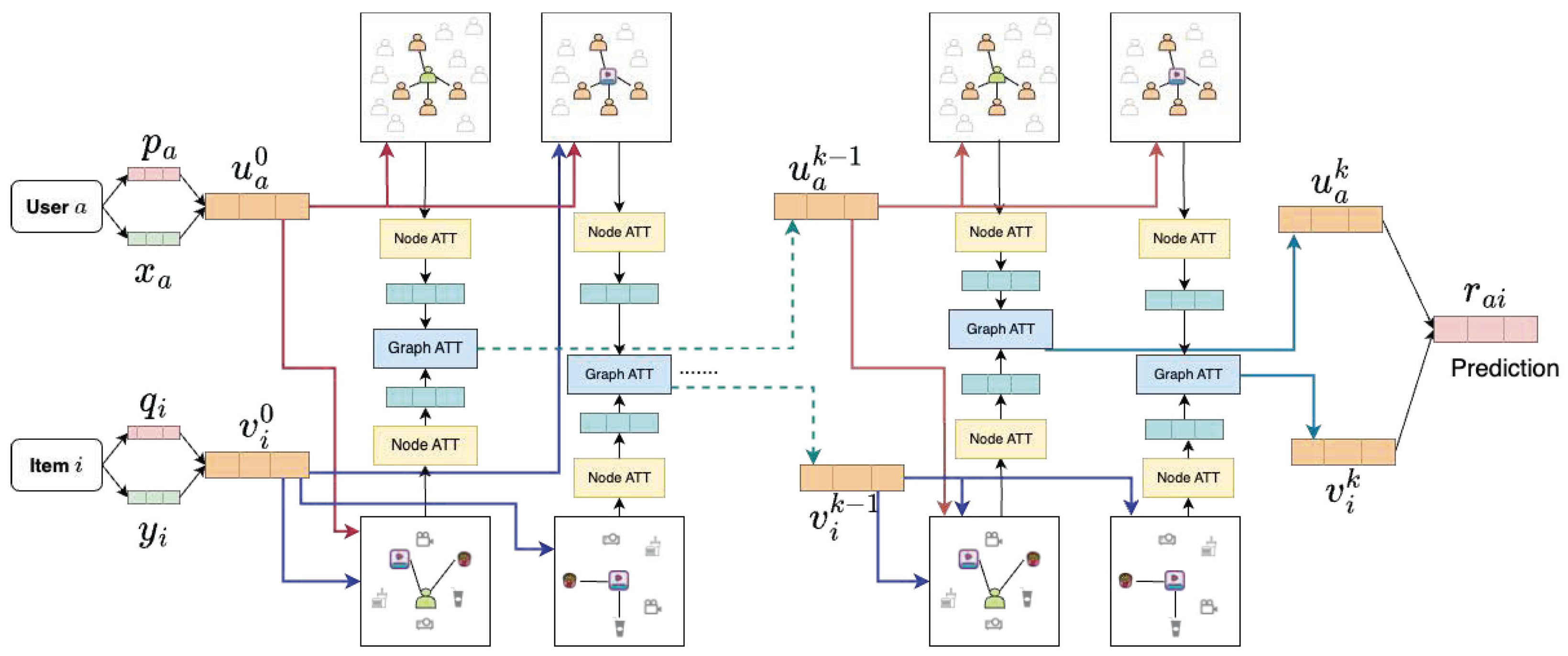
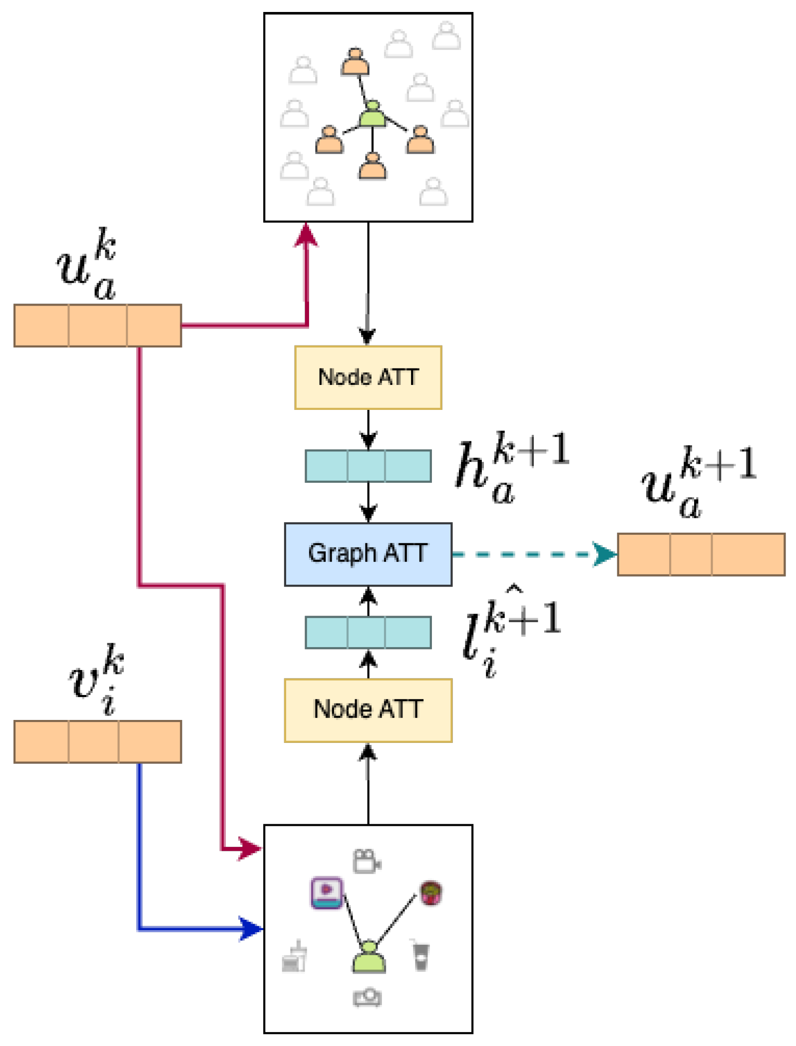
In order to meet the objective of Formula (1), we introduce RelationalNet, a GNN-based architecture that takes as input the utility matrix R as well as the adjacency matrices S and T, and the user and item embeddings X and Y, respectively, to predict the missing ratings ${\widehat{r}}_{ui}$ of $\widehat{R}$. Figure 1 depicts the RelationalNet algorithm architecture, highlighting how each layer is interconnected to produce the final rating for a given pair of user and item. Note that each layer considers four different graphs created from $R,S$, and T matrices. We explain each component of this architecture in what follows.

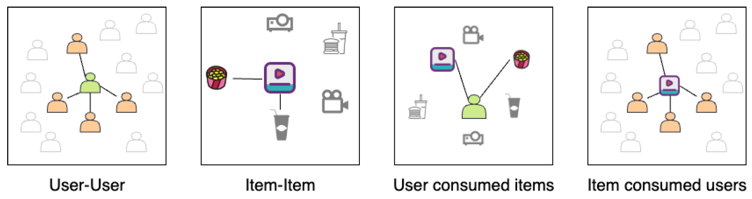
3.2.1. Constructed Graphs

We now review in more detail the four distinct graph structures that our model uses to facilitate the training process for predicting unknown ratings as illustrated in Figure 2. These graph structures encompass the following:

• User–user graph $G_S$: The user–user graph captures the social interactions between users by establishing links between them. This graph emphasizes the significance of user preferences influenced by their social connections. For instance, within the Yelp dataset, if user A follows users B and C, we create directed graph edges (links) from user A to user B and user A to user C.
• Item–item graph $G_T$: The item–item graph establishes links between items that exhibit similarities to each other. This graph captures the relationship between items based on shared characteristics. For example, within the Yelp dataset, if two restaurants serve similar food categories, a link is established between these restaurants.
• User–consumed–items graph $G_R$: The user–consumed–items graph is formed based on the interactions between users and items derived from each user’s past behavior as given from the utility matrix R. It represents the items that a user has interacted with. For example, if user A watches the movies Avengers and Avatar, connections (links) are established between user A and the movie Avengers and between user A and the movie Avatar.
• Item–consumed–users graph $G_R^{\prime }$: The item–consumed–users graph connects items with the users who have interacted with them as given from the utility matrix R. It signifies the users who have engaged with a particular item. For instance, if the movie Avengers is watched by users A and B, links are created between the Avengers movie and user A, as well as between the Avengers movie and user B. Note that graphs $G_R$ and $G_R^{\prime }$ are the same bipartite graph with the emphasis on user nodes and item nodes, respectively.

Compared to existing models, the RelationalNet model introduces the incorporation of item relations through the item–item graph $G_T$ and item–consumed–users graph $G_R^{\prime }$. Similar to how users learn from their neighboring users in the user–user graph $G_S$, items may also learn from their neighboring items. This inclusion of item relations enhances the model’s capacity to capture complex item–item dynamics, thereby improving the quality of recommendations generated by the RelationalNet model.

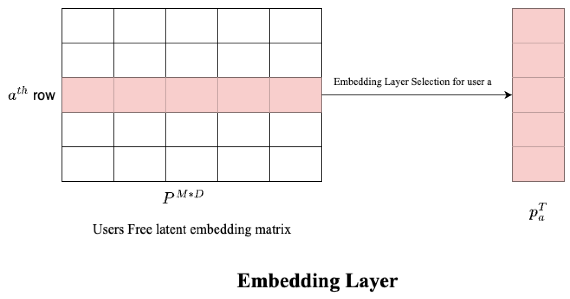
3.2.2. Embedding Layer  [13]

The utilization of embedding layers is commonplace in the field of Natural Language Processing (NLP), as evidenced by numerous works such as [4,25,26]. The embedding layer is part of the hidden layers in a deep neural network, taking high-dimension input and outputs into a lower dimension. RSs utilize this technique to represent users and items with respective free vector encodings.

• Let $P\in R^{m\times D}$ represent the free latent embedding matrices of users with D-dimensions. The embedding layer executes an index selection operation to generate the unrestrained latent vector of the user $p_a$ for user a at ath row. Figure 3 shows that step.
• Similarly, let $Q\in R^{n\times D}$ represent the free latent embeddings matrices of items with D-dimensions. The embedding layer executes an index selection operation to generate the unrestrained latent vector of the item $q_b$ for item b at the bth row.

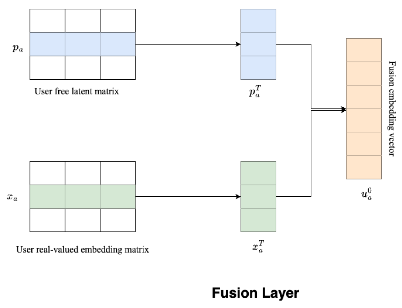
3.2.3. Fusion Layer [13]

The fusion layer merges the latent free vector with the real-valued embedding vector to capture diverse initial interests from the input data. The combination of these two vectors is essential for effective information integration. Figure 1 shows that step; left side before Layer 1.

• The fusion layer processes latent free vectors $p_a$ from the embedding layer and real-valued embedding vectors $x_a$ from input data X for each user a. The output is the users’ initial interests $u_a^0$ across various input types:

  $$u_a^0=g(W_1\times [p_a,x_a])$$

  (2)

  where $W_1$ is a trainable weights matrix, and $g(x)$ is a function of the transformation matrix. Figure 4 shows the fusion layer for the user embedding.
• For each item i, the inputs are the latent free vector $q_i$ and the real-valued embedding vectors $y_i$, and the output is the initial interests $v_i^0$ of the items:

  $$v_i^0=g(W_2\times [q_i,y_i])$$

  (3)

  where $W_2$ is a trainable weights matrix, and $g(x)$ is a function of the transformation matrix.

3.2.4. Node Attention Layer

In GNNs, each node receives and combines features from its neighboring nodes to capture the local structure of the graph. Different types of GNN layers use various aggregation techniques for the message-passing process.

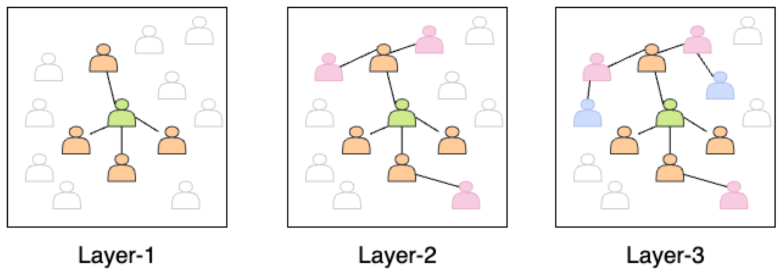
Each of our graphs employs attention from neighboring nodes to enhance each user’s training. This attention can be computed in various ways, such as taking the mean, concatenating it into vectors, or selecting the maximum value from neighboring values. By repeatedly diffusing users’ preferences through propagation in the graph, their preferences are effectively spread out as shown in Figure 5.

• Let each user a have $h_a^k$ as the latent embedding at the $k^{th}$ layer, then the user a latent embeddings for the neighboring nodes in $G_S$ at layer $k+1$ is

  $$h_{Sa}^{k+1}=g(h_b^k|b\in S_a)$$

  (4)

  where $g(x)$ is an attention function, and $Sa$ is the neighborhood of a. The user’s a latent embedding can be trained for layer $k+1$ with the combination of its own $h_a^k$ and of the neighboring latent embeddings $h_{Sa}^{k+1}$:

  $$h_a^{k+1}=\alpha (W^k\times [h_{Sa}^{k+1},h_a^k])$$

  (5)

  where $\alpha (x)$ is a non-linear transformation function similar to DiffNet++.
• Let each item i have $l_i^k$ as the latent embedding at the $k^{th}$ layer, then the item i latent embeddings for the neighboring nodes in $G_T$ at layer $k+1$ is

  $$l_{Ti}^{k+1}=g^{\prime }(l_b^k|b\in T_i)$$

  (6)

  where $g^{\prime }(x)$ is an attention function and $T_i$ is the neighborhood of i. The item i latent embeddings can be trained for layer $k+1$ with the combination of $l_i^k$ and $l_{T_i}^{k+1}$ neighboring latent embeddings:

  $$l_i^{k+1}={\alpha }^{\prime }(W^k\times [l_{Ti}^{k+1},l_i^k])$$

  (7)

  where ${\alpha }^{\prime }(x)$ is a non-linear transformation function similar to DiffNet++.

Similarly, the consumed items by each user and those consumed for each item are trained for k layers using attention.

• Let each user a have ${\tilde{h}}_a^k$ as latent embedding at the $k^{th}$ layer, then the user a latent embeddings for the consumed item nodes in $G_R$ at layer $k+1$ are

  $${\tilde{h}}_{Va}^{k+1}=g({\tilde{h}}_b^k|b\in V_a)$$

  (8)

  where $V_a$ represents the items consumed by user a, and $g(x)$ is a transformation function. The user a latent embeddings can be trained for layer $k+1$ with a combination of ${\tilde{h}}_a^k$ and ${\tilde{h}}_{Va}^{k+1}$ consumed item latent embeddings:

  $${\tilde{h}}_a^{k+1}=\beta ({\tilde{W}}^k\times [{\tilde{h}}_{Va}^{k+1},{\tilde{h}}_a^k])$$

  (9)

  where $\beta (x)$ is a non-linear transformation function.
• Let each item i have ${\tilde{l}}_i^k$ as the latent embedding at the $k^{th}$ layer, then the item i latent embeddings for the consumed user nodes in $G_R^{\prime }$ at layer $k+1$ are

  $${\tilde{l}}_{Si}^{k+1}=g({\tilde{l}}_b^k|b\in S_i)$$

  (10)

  where $S_i$ represents users who consumed item i and $g(x)$ is an attention function. The item i latent embeddings can be trained for layer $k+1$ with a combination of ${\tilde{l}}_i^k$ and ${\tilde{l}}_{S_i}^{k+1}$ consumed users’ latent embeddings:

  $${\tilde{l}}_i^{k+1}=\beta ({\tilde{W}}^k\times [{\tilde{l}}_{Si}^{k+1},{\tilde{l}}_i^k])$$

  (11)

  where $\beta (x)$ is a non-linear transformation function.

Figure 1 shows that step with the use of yellow boxes labeled Node ATT.

3.2.5. Graph Attention Layer

The graph attention layer, depicted in Figure 1 with blue boxes labeled Graph ATT, generates the latent embeddings for each user and for each item using node attention at every layer by a combination of suited graph embeddings.

• For user a, using the graph attention layer at the ${(k+1)}^{th}$ layer to combine the latent embeddings learned from neighboring users $h_a^{k+1}$ and from item consumed users ${\tilde{l}}_i^{k+1}$ for each item i and item latent embeddings from the $k^{th}$ layer, i.e., $v_i^k$, is

  $$u_a^{k+1}=ML{P}_2([h_a^{k+1},ML{P}_1([{\tilde{l}}_i^{k+1},v_i^k])])$$

  (12)

  where $ML{P}_1,ML{P}_2$ are the multi-layer perceptrons used to learn the complex relationship between social relations and item embeddings. Figure 6 shows an example of this step.
• For item i, using the graph attention layer at the ${(k+1)}^{th}$ layer to combine the latent embeddings learned from neighboring items $l_i^{k+1}$ and from users consumed item ${\tilde{h}}_a^{k+1}$ for each user a and item latent embeddings from $k^{th}$ layer, i.e., $u_a^k$, is

  $$v_i^{k+1}=ML{P}_2([l_i^{k+1},ML{P}_1([{\tilde{h}}_a^{k+1},u_a^k])])$$

  (13)

  where $ML{P}_1,ML{P}_2$ are the multi-layer perceptrons used to gain an understanding of the intricate connections between item relations and user embeddings.

3.2.6. Prediction Layer

To predict a user’s rating for an item ${\widehat{r}}_{ai}$, we consider the latent embedding of each user a from the final graph attention layer of Equation (12) denoted as $u_a^k$ at the $k^{th}$ layer after the repeated diffusion of neighbors from Equation (4). Similarly, for every item i, we consider its latent embeddings from the graph attention layer Equation (13) denoted as $v_i^k$:

$${\widehat{r}}_{ai}={(v_i^k)}^T\times u_a^k$$

(14)

3.2.7. Loss Function

Our focus is on the implicit feedback of users. In line with the commonly used ranking-based loss function in Bayesian personalized ranking [27], the loss function based on pairwise ranking for optimization purposes is defined as

$$minimize(L(R,\widehat{R}))=\sum _{a=1}^M\sum _{i\in D_a}^N\sigma ({\widehat{r}}_{ai}-r_{ai})$$

(15)

where $\sigma (x)$ is a sigmoid function. $D_a$ represents the (previously) rated items of user a. To implement it, we utilize TensorFlow to execute the suggested model. RelationalNet optimizes the model parameters using a mini-batch Adam optimizer.

3.2.8. Time Complexity

Following a similar analysis as in DiffNet++ [13], the additional time cost lies in the influence and interest diffusion layers for users and items, when compared to the classical matrix factorization-based algorithms. Given m users, and n items and diffusion depth of K, let us denote the maximum degree of $G_S$ by $maxDe{g}_S$, the maximum degree of $G_T$ by $maxDe{g}_T$, the maximum items per user in $G_R$ by $maxI$, and the maximum users per item in $G_R^{\prime }$ by $maxU$. At each layer, we need to update the embeddings using Equations (12) and (13). As noted, in practice, the MLP layers are two, so the time cost for the graph attention modeling is $O(D\{m(maxDe{g}_S+maxI)+n(maxDe{g}_T+maxU)\})$, where D is the dimension of the embeddings. Since there are K layers, the total additional time complexity of our algorithm is $O(KD\{m(maxDe{g}_S+maxI)+n(maxDe{g}_T+maxU)\})$. Additionally, we have practically that $maxDe{g}_S,maxU<<m$ and $maxDe{g}_T,maxI<<n$, thus being almost linear to the number of users and items.

4. Experimental Evaluation

4.1. Dataset

Similar to previous work, we employed the Yelp dataset [28] to evaluate our approach. The Yelp dataset is ideal, as it includes not only ratings but also additional information on businesses, reviews, check-ins, tips, and users. It contains data on various types of businesses, including restaurants, bars, and cafes. These details include their names, addresses, phone numbers, categories, ratings, operational hours, and reviews. Individual users provide a rating of 1 to 5 (5 being the best) stars and compose written evaluations for businesses. Most importantly, the dataset incorporates social network information, such as the followers of each Yelp user and the number of fans subscribed to a business. To analyze the Yelp dataset, a preprocessing step is performed by converting star ratings of 3 or higher to a rating of 1, indicating a positive sentiment towards the business, and ratings below 3 are converted to 0, indicating negative sentiment. To obtain insights from the written reviews, the gensim tool and the Word2vec [29] model are employed to generate the embedding of each word. By doing so, it becomes possible to produce a feature vector for each user by computing the mean of the trained word vectors that are correlated to their reviews. A similar process is employed to create feature vectors for every item (business). The feature vectors for both users and items serve as inputs to the model, denoted as X and Y, respectively.

Using the user followers’ information, we create the user–user graph. In this graph, a link is established between user a and user b if user a follows user b, and the link is assigned a weight of 1, which is used for creating the social adjacency matrix S. The dataset also contains information on the items (businesses) and their categories. Businesses with at least seven common categories are considered similar, and a link is assigned between them to create a business–business (item–item) adjacency matrix T. The user–user and item–item inputs S and T are respectively used for creating the graphs $G_S$ and $G_T$ for the neural network to capture the graph relationships.

During the training and testing process, the dataset is filtered to exclude information that may not be reliable or useful. Users with inadequate information, such as those with less than ten reviews or ten followers, are removed from the dataset. By applying these filters, the dataset is refined to ensure that only relevant and reliable information is utilized for the analysis.

Table 1. Yelp dataset.

Dataset	Yelp
Users	1,987,897
Businesses	150,346
Reviews	6,990,280
Filtered Users	15,519
Filtered Businesses	24,648
Filtered Reviews	815,777
Social Links (user–user)	836,186
Item links (item–item)	196,010
Reviews Sparsity	0.213%
Avg no. of ratings/user	37
Median no. of ratings/user	22

summarizes the statistics of the original Yelp dataset as well as the filtered one used in our experiments.

4.2. Training Setup

After preprocessing, the dataset is divided into three distinct subsets—the training, validation, and test datasets, using a ratio of 7:1:2, respectively. At the initialization of the model, there are fixed input values provided for various parameters, such as the user feature matrix X, items feature matrix Y, user–consumed–items graph $G_R$, item–consumed–users graph $G_R^{\prime }$, user–user graph $G_S$, and item–item graph $G_T$. The fixed input values are utilized in various layers of the training model. In the training process, the hyperparameters are fine-tuned using the validation dataset.

During each epoch, different mini-batches of users with varying sizes (100, 250, 500, and 1000) are tested, and it is found that a batch size of 500 yields comparatively better results than other batch sizes. The Adam optimizer is utilized to optimize the model, with an initial learning rate of [$0.001$, $0.0025$, $0.005$] and a decay learning rate to minimize the loss function given by Equation (15). To train the model to be unbiased, a certain number of false negative ratings are added for each user from randomly selected unrated items.

The GNN models utilize the depth parameter K to gauge the impact of diffusion on the overall model (as shown in Equations (12) and (13)). To evaluate the performance of the model, it is trained with different values of $K=2,3$. The size of the user and item-free embeddings, denoted as D, is determined by the number of dimensions in the fusion layer as well as the subsequent diffusion layers. For the fusion layers, we use a sigmoid function as the non-linear function $g(x)$ to transform each value into the range (0, 1) (as shown in Equations (2) and (3)). The output size of each layer is set to $D=64$ dimensions.

4.3. Performance Metrics

We validate our model and evaluate it against SOTA RS algorithms and models using the Root Mean Square Error (RMSE) metric. Using this as a first indicator on which models perform the best overall, we then proceed to evaluate in more detail the model’s ability to generate accurate top-n recommendations. The two main metrics used for this purpose are hit rate (HR) and Normalized Discounted Cumulative Gain (NDCG).

4.3.1. Root Mean Square Error (RMSE)

First, we calculate RMSE over the entire set of predictions. RMSE is a metric that penalizes high differences between the predicted ratings ${\widehat{r}}_i$ and the ground truth rating $r_i$ over all items i in the test (or validation) set. It is defined as follows:

$$RMSE=\sqrt{\frac{{\sum }_{i=1}^N{({\widehat{r}}_i-r_i)}^2}{N}}$$

(16)

where N is the total number of predicted ratings.

RMSE is a good indicator of how well the system performs overall and is broadly used for validation (hyperparameter tuning, model selection, etc.). However, as it penalizes equally both high and low rating predictions, and is applied over the entirety of the validation/test data, it is not a good indicator of the accuracy of the top-n recommendations the system generates, compared to HR and NDCG.

4.3.2. Hit Rate (HR)

HR is a metric used to evaluate the performance of the model by calculating the percentage of times that at least one item from the test set of a user was recommended in the top-n recommendations suggested by the model:

$$HR@n=\frac{\mathrm{Number}\mathrm{of}\mathrm{users}\mathrm{with}\mathrm{at}\mathrm{least}\mathrm{one}\mathrm{hit}\mathrm{in}\mathrm{top}\text{-}n}{\mathrm{Total}\mathrm{number}\mathrm{of}\mathrm{users}}$$

(17)

Hit rate $HR@n$ for a top-n recommendation list is defined as follows [30]:

$$HR@n=\frac{|H_u|}{m}$$

(18)

where $H_u=1$ (i.e., a “hit”) when the algorithm manages to recommend at least one item that was in the user’s original list (test set), and 0 otherwise; n is the size of the recommendation list considered; and m is the total number of users in the test set. Essentially, HR assesses whether the model is able to recommend at least one relevant item to the user.

For example, let us consider a test set of 100 users and their corresponding ground truth sets of movies. The RS generates a list of top-5 movie recommendations for each user. After evaluating the recommendations, it is found that 30 users have at least one recommended movie in their ground truth sets. In this case, the hit rate would be calculated as $30/100=0.3$ or $30\%$.

A higher hit rate serves as an indicator of the effectiveness of an RS, as it suggests that the system is successfully recommending items that match users’ preferences. However, it is essential to recognize that the hit rate metric solely focuses on whether the recommended items are present in the user’s ground truth set, without considering their ranking or relevance. As a result, it is common practice to complement the hit rate with other evaluation metrics to obtain a more comprehensive assessment of the performance of the RS. By incorporating additional metrics, the evaluation process gains insights into the system’s ability to provide accurate and highly relevant top-n recommendations to users.

4.3.3. Normalized Discounted Cumulative Gain (NDCG)

Normalized Discounted Cumulative Gain (NDCG) evaluates the quality of the recommended items’ ranking. This metric accounts for the relevance of items based on their position in the recommendation list, with items at higher positions being deemed more relevant. The metric is normalized based on the ideal DCG (Discounted Cumulative Gain). The ideal DCG represents the cumulative gain of the perfectly ordered items that are most relevant to each user.

The formula for Normalized Discounted Cumulative Gain (NDCG) is:

$$NDCG@n=\frac{DCG@n}{IDCG@n}$$

(19)

where n represents the position in the recommendation list. The Discounted Cumulative Gain (DCG) is defined as:

$$DCG@n=\sum _{i=1}^n\frac{2^{re{l}_i}-1}{{log}_2(i+1)}$$

(20)

where $re{l}_i$ is the score that indicates how relevant the item recommended at position i is, and IDCG (Ideal Discounted Cumulative Gain) is the DCG score of the ideal (i.e., ground truth) list of recommended items. The higher the NDCG score (closer to 1), the better the recommender system is performing in terms of providing relevant and well-ranked recommendations.

In this paper, HR and NDCG are evaluated on the test data to determine how well the models perform. By utilizing these top-n metrics, we can effectively gauge the ability of the model to make accurate recommendations and compare the effectiveness of different models.

4.4. Experimental Results

We first evaluate RelationalNet against four SOTA social RSs using RMSE, namely SocialMF [24], GraphRec [11], and Diffnet++ [13]. The results are shown in

Table 2. Results metrics: Root Mean Square Error (RMSE).

Model	RMSE
SocialMF [24]	2.1990
GraphRec [11]	0.6640
Diffnet++ [13] (GNN Layers K = 2)	0.1676
Diffnet++ [13] (GNN Layers K = 3)	0.1668
RelationalNet Model (GNN Layers K = 2)	0.1701
RelationalNet Model (GNN Layers K = 3)	0.1674

. It is worth mentioning that there are considerable variations between the metrics obtained by GraphRec and the other models. Specifically, while GraphRec predicts ratings on a scale of 1–5, the other models predict whether the user likes an item or not, with binary values of 1 or 0. Hence, comparing the performance of these models based on the same metric can be challenging due to significant differences in the rating scales. Nevertheless, RelationalNet and Diffnet++ clearly outperformed the other two systems, with the three-layer GNN architecture yielding slightly better results for both models. We therefore focused the rest of our experimental evaluation on those two models (four variations).

To ensure fairness in our evaluation, we followed a similar evaluation methodology, using identical datasets and evaluation metrics as in Diffnet++ [13]. Specifically, the Yelp datasets were used, and the model was evaluated using HR and NDCG metrics.

Table 3. Hit rate (HR) for top-5, top-10, and top-15 recommendations.

Model	HR (5)	HR (10)	HR (15)
Diffnet++ [13] (GNN Layers K = 2)	0.2722	0.3136	0.3634
Diffnet++ [13] (GNN Layers K = 3)	0.2376	0.2772	0.3320
RelationalNet Model (GNN Layers K = 2)	0.2946	0.3288	0.3739
RelationalNet Model (GNN Layers K = 3)	0.2840	0.3218	0.3694

presents the results for the HR metric of RelationalNet and Diffnet++ with various combinations of hyperparameters (number of layers). RelationalNet, consisting of a two-layer GNN, gives the best results. Both variations of the RelationalNet model outperform those of Diffnet++ up to 24% for the top-5 recommendations, with an average overall improvement of 11.8%. The analysis revealed that increasing the number of layers led to a decrease in the performance of the recommender system, a pattern that is observed both for the proposed RelationalNet model and the Diffnet++ model.

Table 4. Normalized Discounted Cumulative Gain (NDCG) for top-5, top-10, and top-15 recommendations.

Model	NDCG (5)	NDCG (10)	NDCG (15)
Diffnet++ [13] (GNN Layers K = 2)	0.4822	0.5167	0.5267
Diffnet++ [13] (GNN Layers K = 3)	0.4573	0.4924	0.5044
RelationalNet Model (GNN Layers K = 2)	0.5058	0.5347	0.5416
RelationalNet Model (GNN Layers K = 3)	0.4972	0.5283	0.5376

shows the results for the NDCG metrics for the different models, and again the RelationalNet model with two layers has the best performance. We observe that both RelationalNet variations perform better than those of Diffnet++ for all sizes of top-n recommendation lists with up to 10% improvement for top-5 recommendations and an average overall improvement of 6.2%.

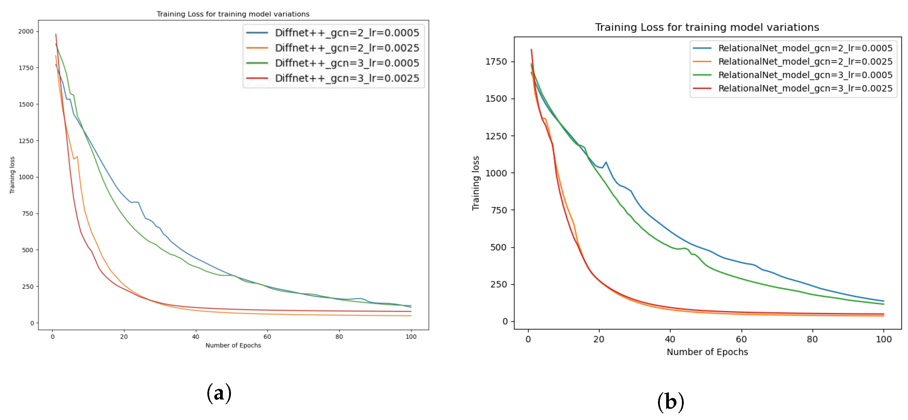
Figure 7a,b illustrate the comparison of the model’s training loss with different learning rates to analyze their performance under various hyperparameters. The visual representation of the loss function enables us to evaluate the model’s convergence rate. These figures reveal that a learning rate of $0.0025$ leads to a smoother decrease in training loss than a learning rate of $0.005$, indicating that the former results offer better convergence. Moreover, the RelationalNet model outperforms the Diffnet++ model in terms of training loss for most learning rates, indicating its ability to learn from input data effectively and suggesting that it can achieve higher accuracy than the Diffnet++ model.

Our findings illustrate the efficacy of the RelationalNet model in tackling the social recommendations generation problem. RelationalNet has achieved accurate user preference prediction in various (realistic) lengths of top-n recommendation lists and outperformed several SOTA social recommender systems. The outcomes indicate that integrating GNN layers to facilitate interest and influence diffusion leads to an enhancement in the recommendation accuracy. The RelationalNet model can potentially enhance the recommendation accuracy in social RSs and can be effectively used in real-world applications.

4.5. Ablation Study

We perform an ablation study to explore whether the item–item graph $G_T$ that we create, such that similar items are connected, enriches our embeddings. To evaluate this hypothesis, we employ an item–item graph $G_T^{*}$ that is created by connecting items randomly. We achieve that by replacing every edge $e=(v,u)\in G_T$ (positive edge) with a negative edge $e^{*}$ that connects v with a node $u^{*}$ that is not in the neighborhood of v. We then reduce the degree of each node by 10 but cap the minimum degree at 1. The ablation results, shown in

Table 5. Ablation study.

Layers	Metric	RelationalNet with ${\mathit{G}}_{\mathit{T}}$ (Table 3 and Table 4)	RelationalNet with ${\mathit{G}}_{\mathit{T}}^{*}$ (Ablation)
k = 3	RMSE	0.1674	0.1855
k = 2	HR@5	0.2946	0.2901
k = 2	HR@10	0.3288	0.3243
k = 2	HR@15	0.3739	0.3714
k = 2	NDCG@5	0.5058	0.5036
k = 2	NDCG@10	0.5347	0.5324
k = 2	NDCG@15	0.5416	0.5404

, are consistent with our hypothesis that the item–item graph $G_T$ enriches our model, as using an item–item graph with negative edges and fewer connections decreases the performance of the model in terms of RMSE, HR@5/10/15 and NDCG@5/10/15. It is important to note that the greatest difference between our experimental results and the ablation results is in HR@5 and NDCG@5, while HR@10/15 and NDCG@10/15 are closer. This is expected for the specific dataset since after preprocessing, there exist many items that have fewer than 10 ratings. When the number of training samples is less than the number of predicted ratings, the hit rate and NDCG values have less relevance.

5. Conclusions and Discussion

This paper proposes RelationalNet, a novel neural influence and diffusion algorithm for social recommendations based on Diffnet++ [13]. RelationalNet improves upon Diffnet++ with the addition of item–item and item–user interactions modeled as graphs used in the GNNs. By incorporating not only user–user relations in the form of the social graph (similar to other social recommender systems) but also item–item relations that are independent of any user interactions, RelationalNet addresses the cold-start problem of little or no user–item ratings. Furthermore, RelationalNet utilizes a multi-layer diffusion network that employs graph attention to combine graph and node-level representations, managing to capture the latent features of each graph. The experimental evaluation showed that the RelationalNet algorithm achieves better performance in generating top-n recommendations (with a $11.8\%$ improvement of HR and $6.2\%$ improvement of NDCG on average) as opposed to the current SOTA and predecessor, Diffnet++, showing the potential of such extensions that enhance the input with additional connections.

There is still significant scope to explore, like the different mechanisms for forming connections between items, calculating user and item similarities, exploring higher-order connections [31,32] instead of edges, and investigating graph reasoning algorithms to learn users’ preferences better. In addition, we plan to leverage our previous work on influential users [2,23,33,34] to refine the user–user similarities and create neighborhoods of influence. Perhaps one of the main shortcomings of the proposed approach is the overhead that is introduced by adding one additional graph and expanding the social network beyond direct neighbors, as the RelationalNet algorithm was $25\%$ slower than the DiffNet++ algorithm. The biggest cost factor to consider if we want to make our algorithm scalable is to restrict the attention modules in the nodes and in the graphs. We can achieve this by reducing the dimensions of the embeddings for the user and item, respectively. One of the future ideas is to use subgraph sampling for the training. However, selecting representative subgraphs that will preserve good graph characteristics needs further investigation, especially in our case, where we have four graphs. While using subgraph sampling will increase the scalability of the model, this comes with the cost of accuracy and expressability of the model.

Overall, the RelationalNet algorithm provides a significant step forward in social recommendation systems by taking advantage of social connections, item correlations, and leveraging the power of GNNs.