
Research on a Classification Method for Strip Steel Surface Defects Based on Knowledge Distillation and a Self-Adaptive Residual Shrinkage Network


Abstract
:1. Introduction
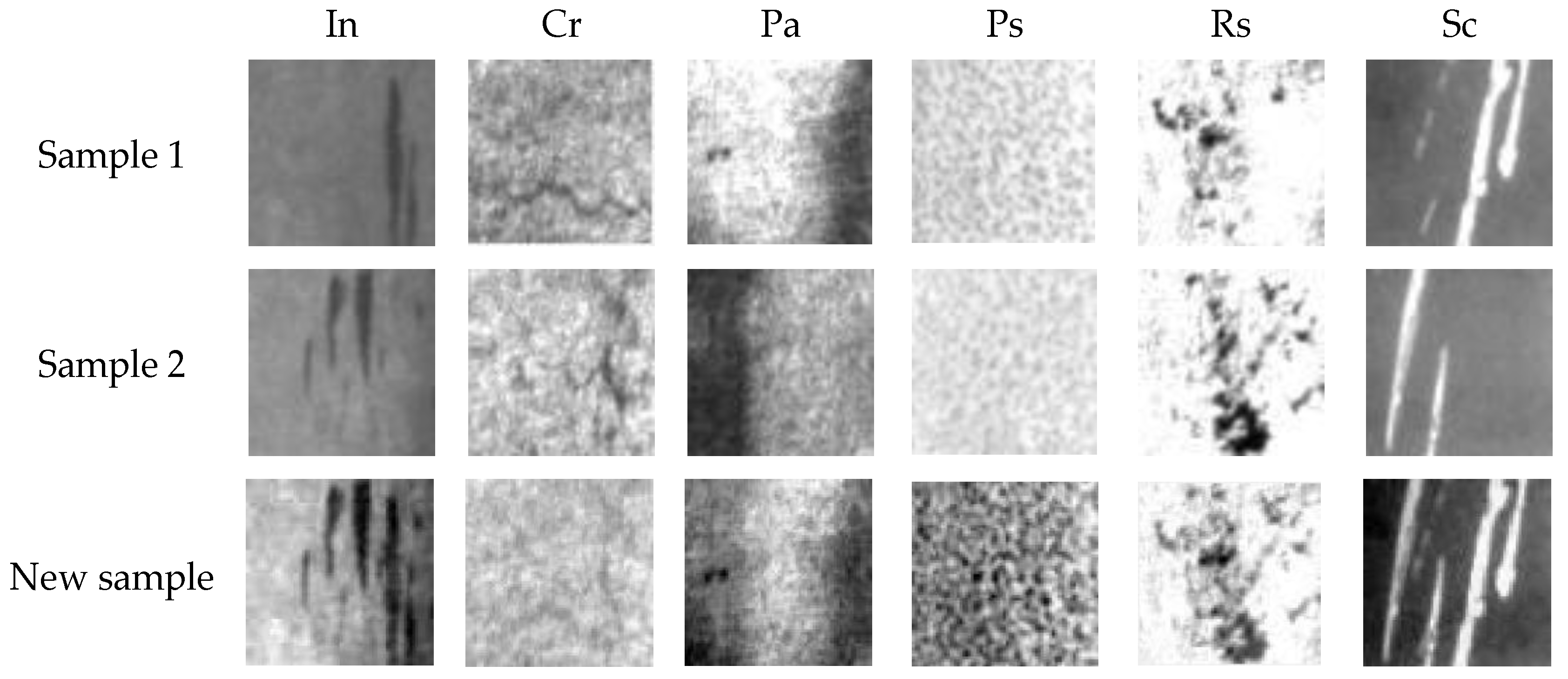
- In the aspect of data enhancement, aiming at the shortage of defect samples in a single production line, a data enhancement method of image mosaic fusion is proposed to improve the matching degree between the model and the data. Aiming at the problem of insufficient defect samples across production lines, an image generation method based on Cycle GAN is proposed to realize the cross domain conversion of defect samples. Compared with the limitations of [8,9,10,11], this method solves the problem of insufficient strip steel defect samples from two angles;
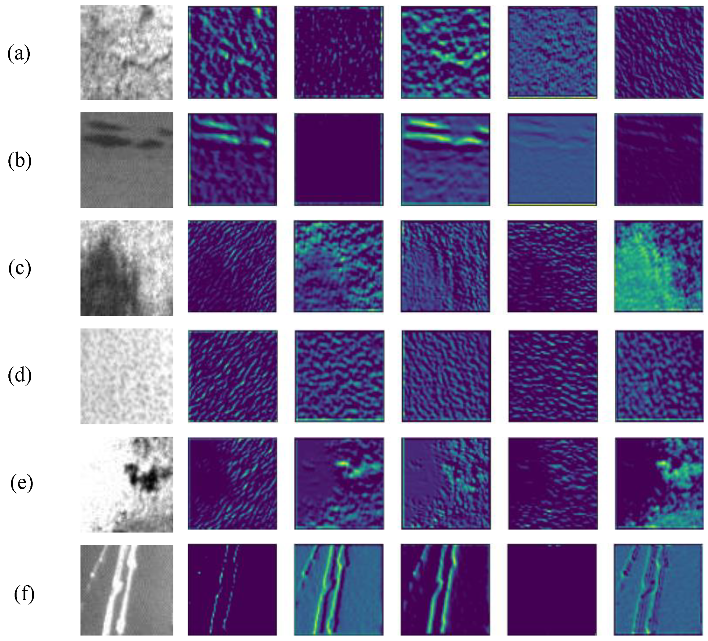
- In terms of feature extraction, based on the integration of the attention mechanism [7], a new backbone network: the self-adaptive residual shrinkage network (SARSN) is proposed to solve the difficulty of image fine-grained feature extraction through a soft threshold and the channel attention mechanism;
- For unbalanced samples, a new adaptive loss function is designed to manage the sample categories separately to achieve a balance between classes to improve the accuracy of the classification model. Compared with the existing methods [12,13], this method is better at handling interclass differences and reduces the sensitivity of the model to data;
- In terms of model deployment efficiency, compared with the literature [6], this method focuses on optimizing the network structure through knowledge distillation and transferring the generalization performance of a large-scale network model to a small-scale lightweight network While ensuring the real-time performance of the classification network, the classification accuracy is 4.3% higher than that in the literature [9];
- Finally, this paper quantifies the evaluation index of strip steel defects by image processing technology and designs a GUI interface that is convenient for users to operate.
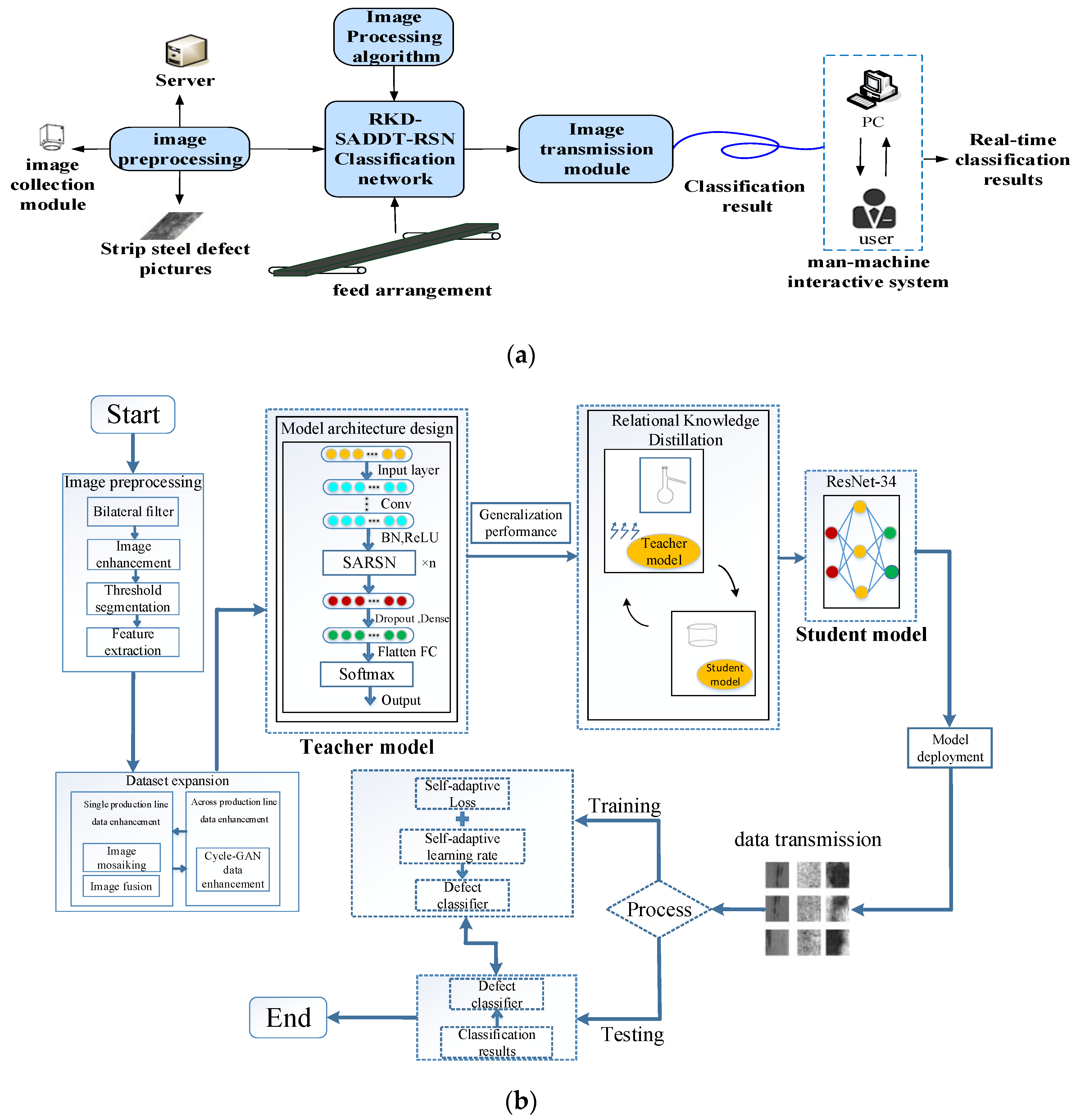
- The organization of the other sections of this paper is as follows: the second part is the theoretical description of the relevant methods. Section 2.1 presents the deployment of the whole algorithm and the algorithm design process. Section 2.2 describes the principle of Cycle GAN data enhancement. Section 2.3 introduces the design process of each part of the feature extraction backbone network. Section 2.4 puts forward the theoretical basis of structured relational knowledge distillation. The third part is the description of the experimental process. Section 3.1 introduces the image preprocessing process; Section 3.2 verifies the performances of the teacher model and student model, respectively. Comparative experiments are carried out in Section 3.2.3 and Section 3.2.4. Finally, combined with an image processing algorithm, the defect evaluation index is proposed, and the GUI operation interface is designed. The fourth part presents the conclusion and prospects.
2. The Proposed Theory
2.1. Model Deployment Process and Algorithm Structure Design
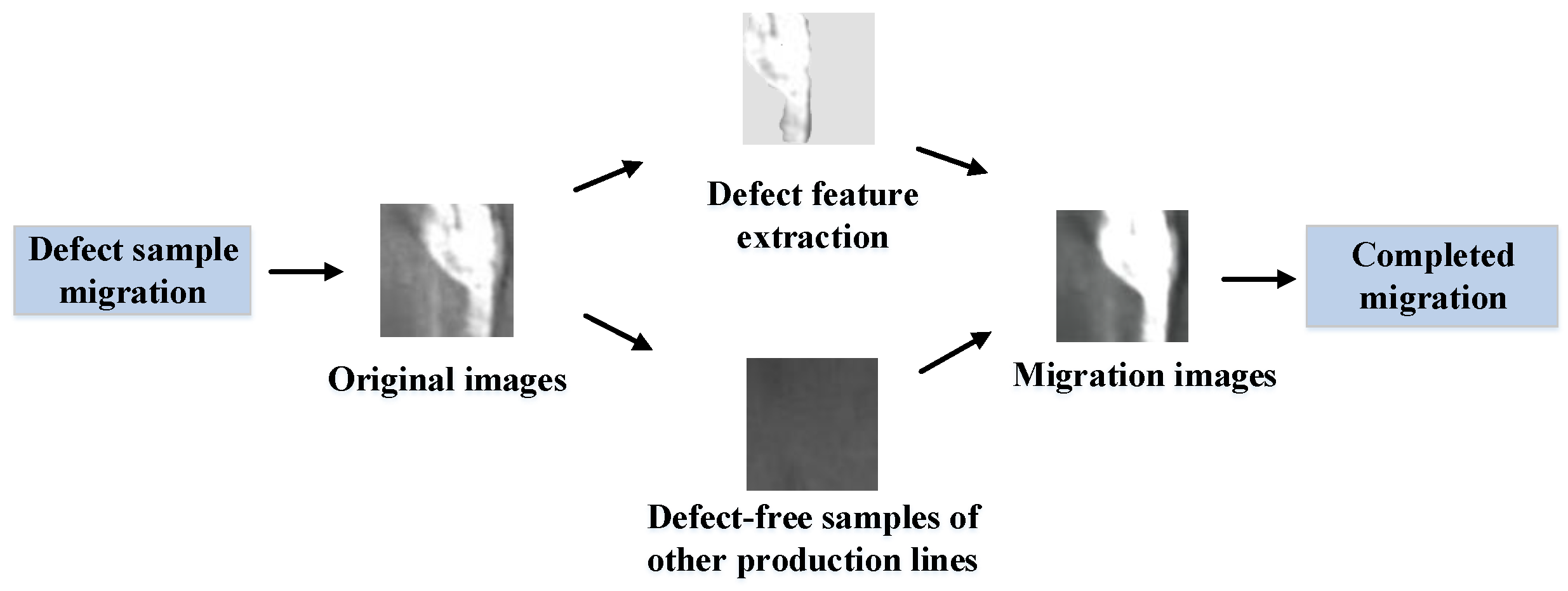
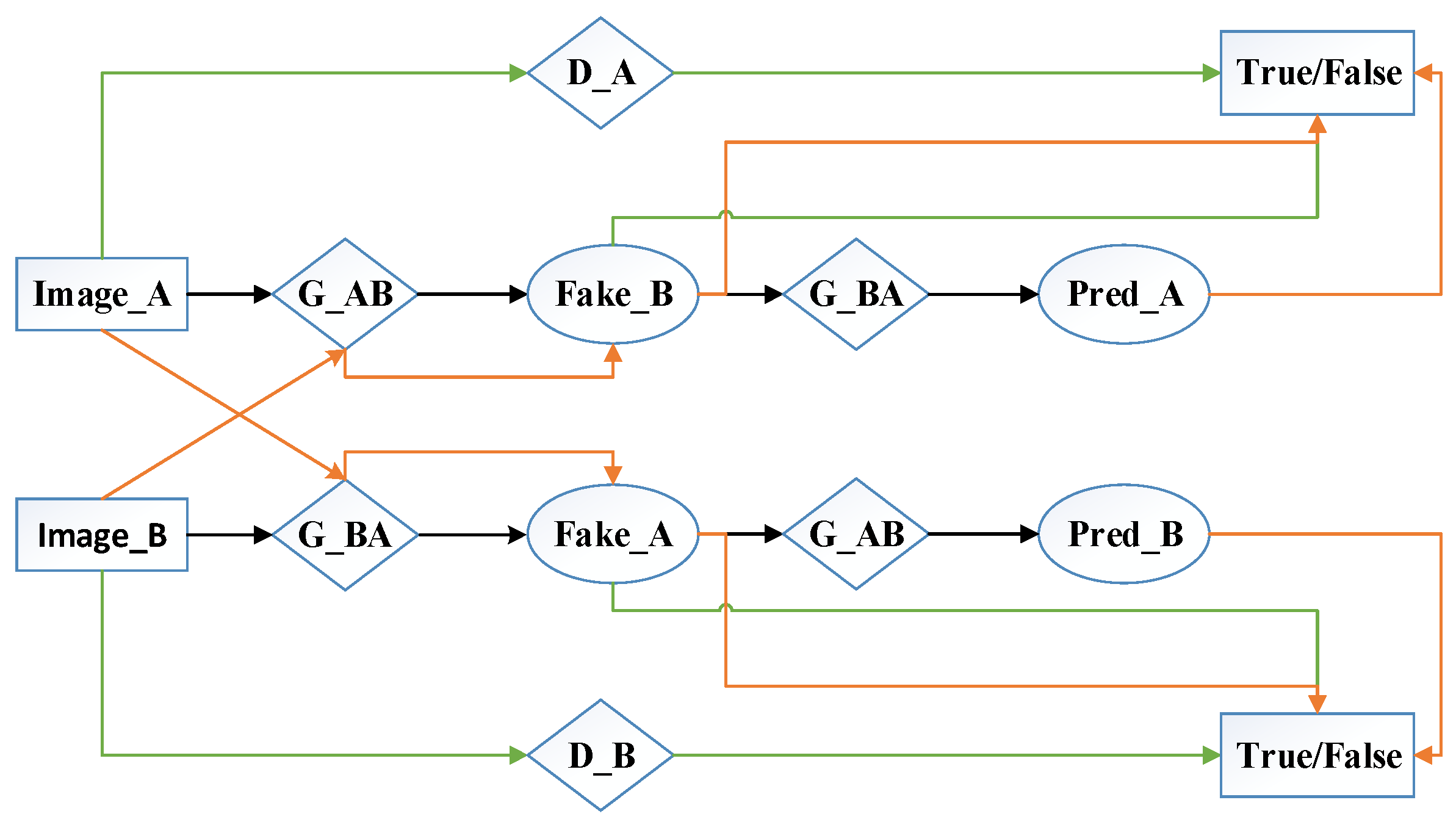
2.2. Image Cross-Domain Conversion: Data Enhancement Based on Cycle GAN
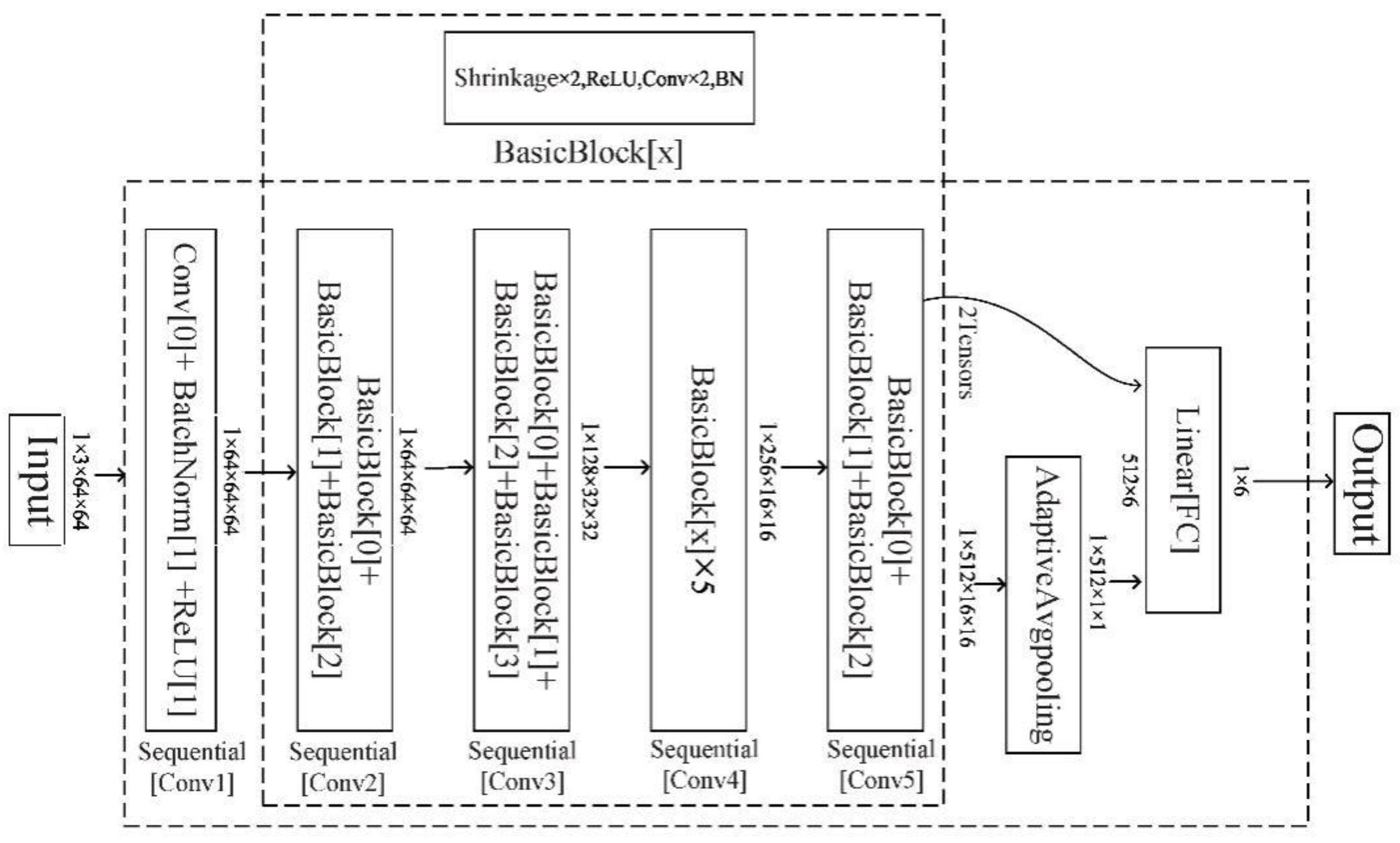
2.3. Classification Network Structure Design
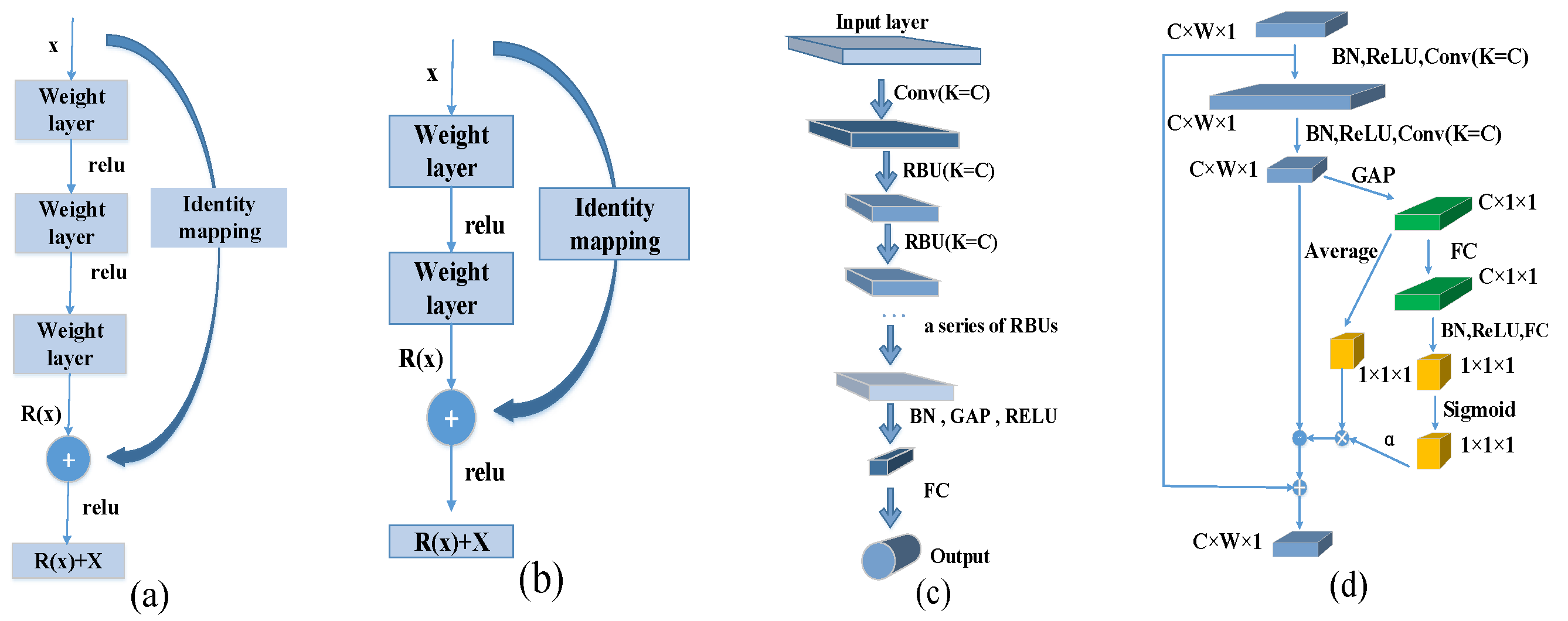
2.3.1. Deep Residual Shrinkage Network
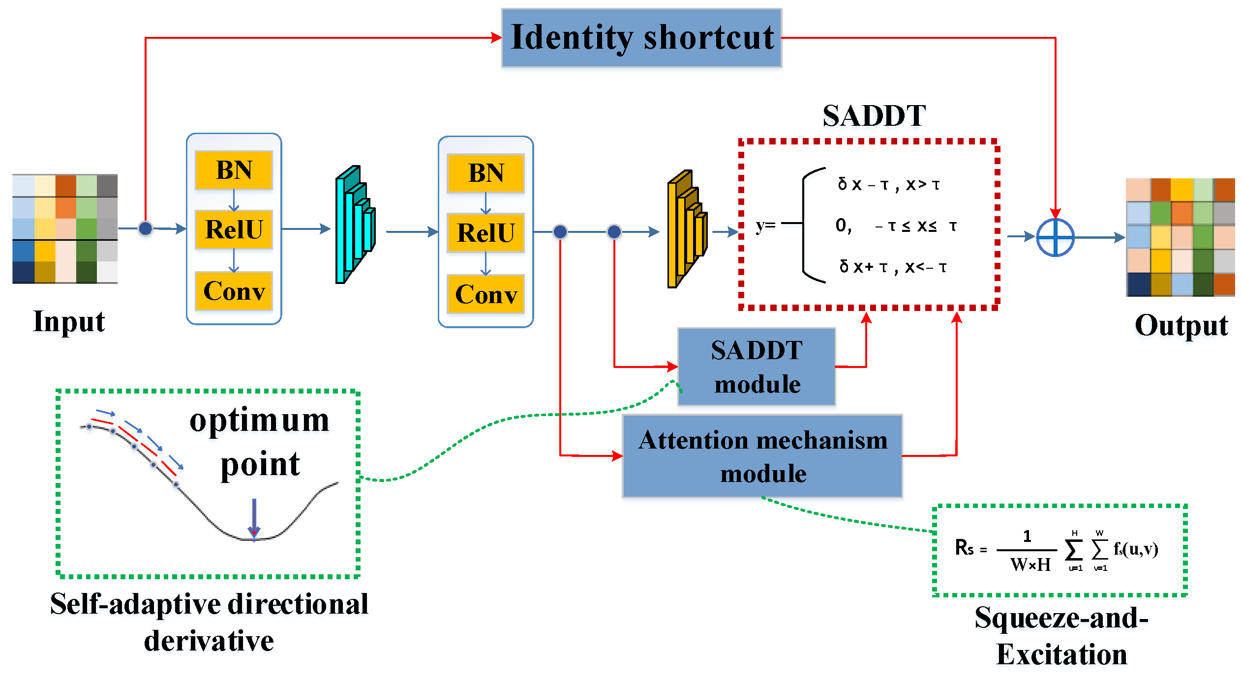
2.3.2. The Proposed Self-Adaptive Residual Shrinkage Network (SARSN)
- (1)
- Attention mechanism and squeeze-and-excitation networks:
- (2)
- Self-adaptive directional derivative threshold
- (3)
- Self-adaptive loss function
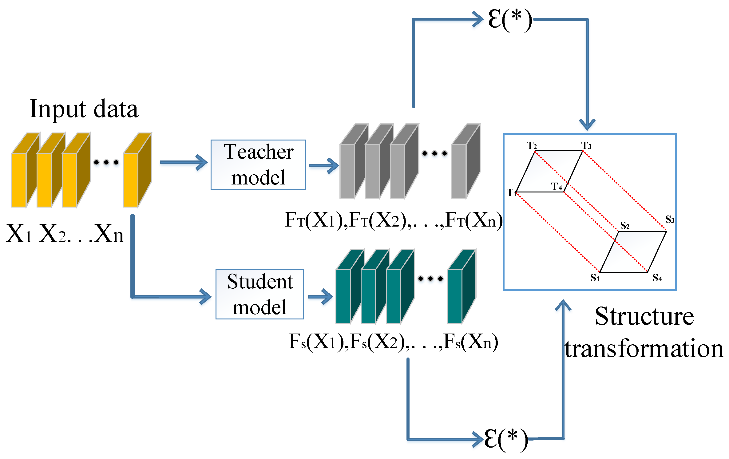
2.4. Knowledge Distillation
3. Experimental Results
3.1. Experimental Data Processing
3.1.1. Image Preprocessing
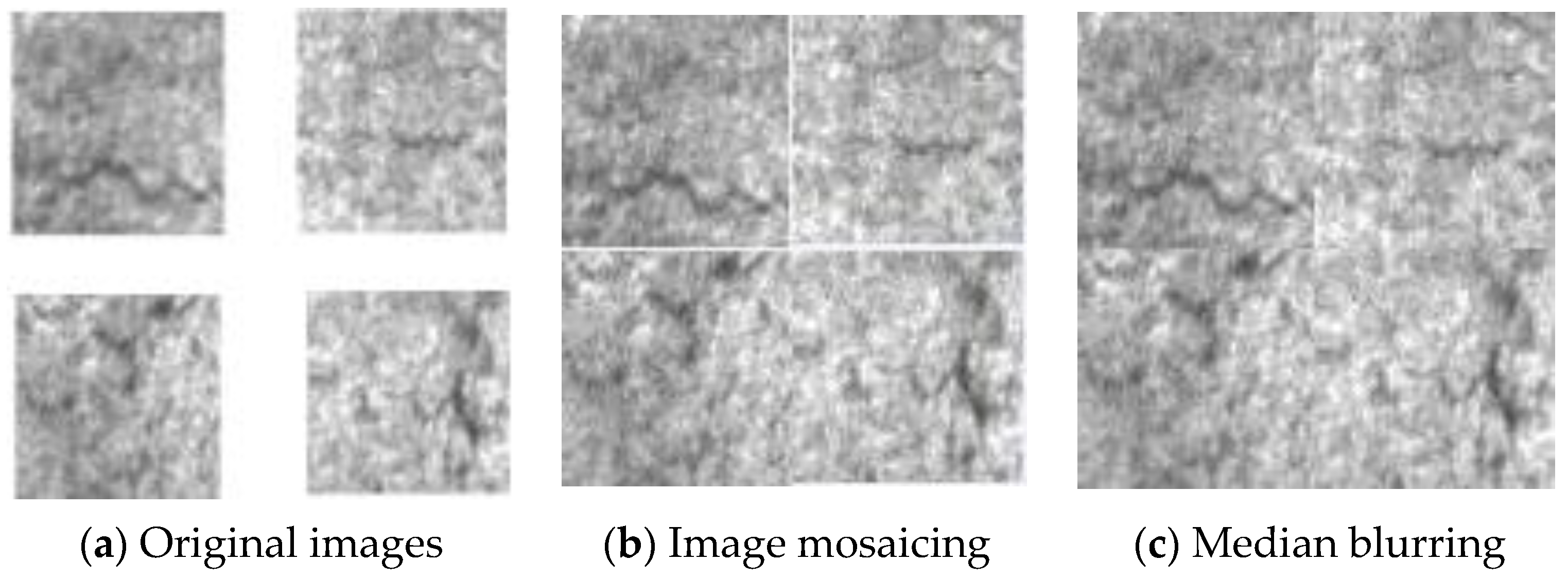
3.1.2. Image Mosaicing and Fusion
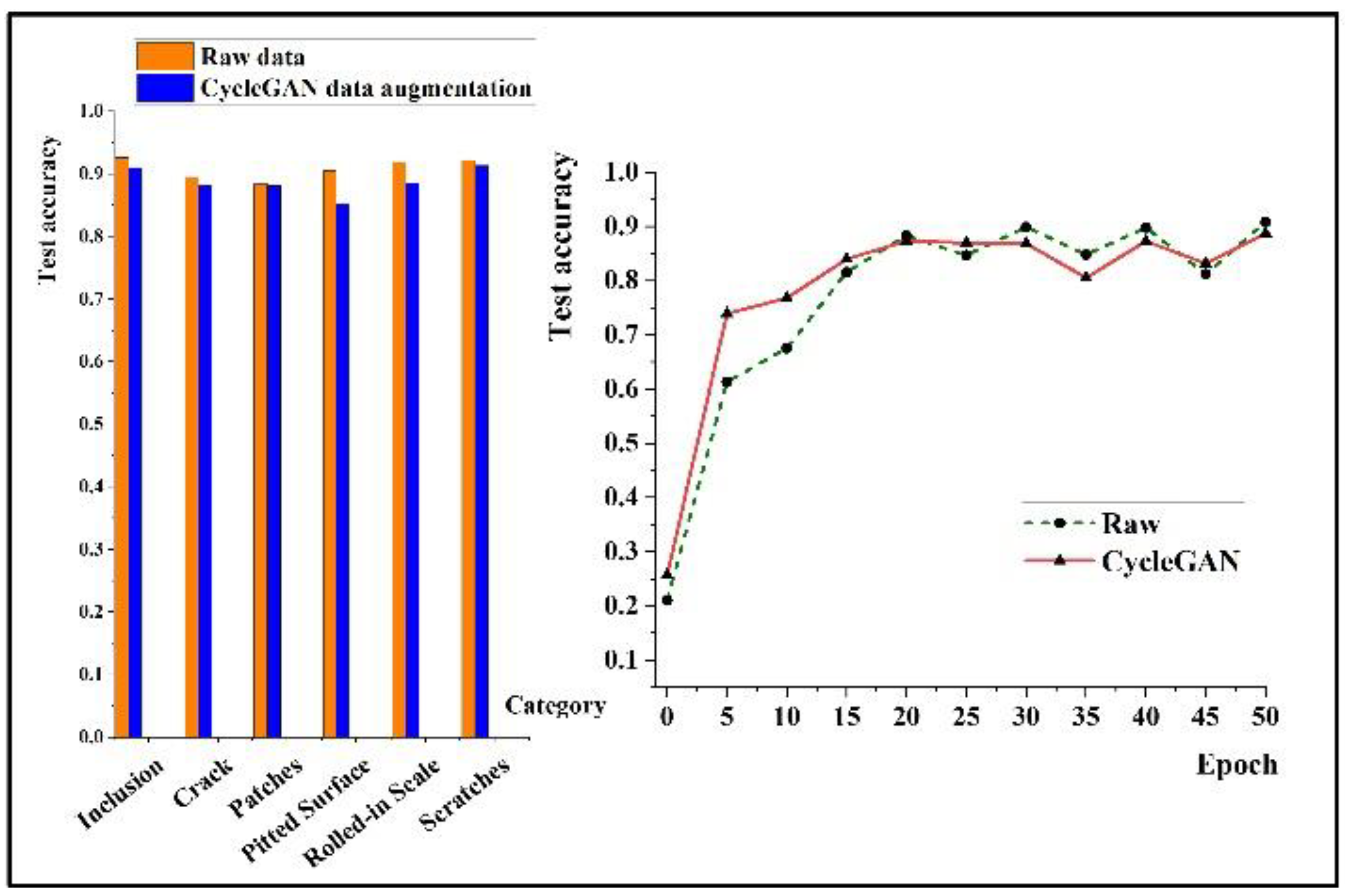
3.1.3. Cycle GAN Data Enhancement Experiment
3.2. Model Verification Experiment
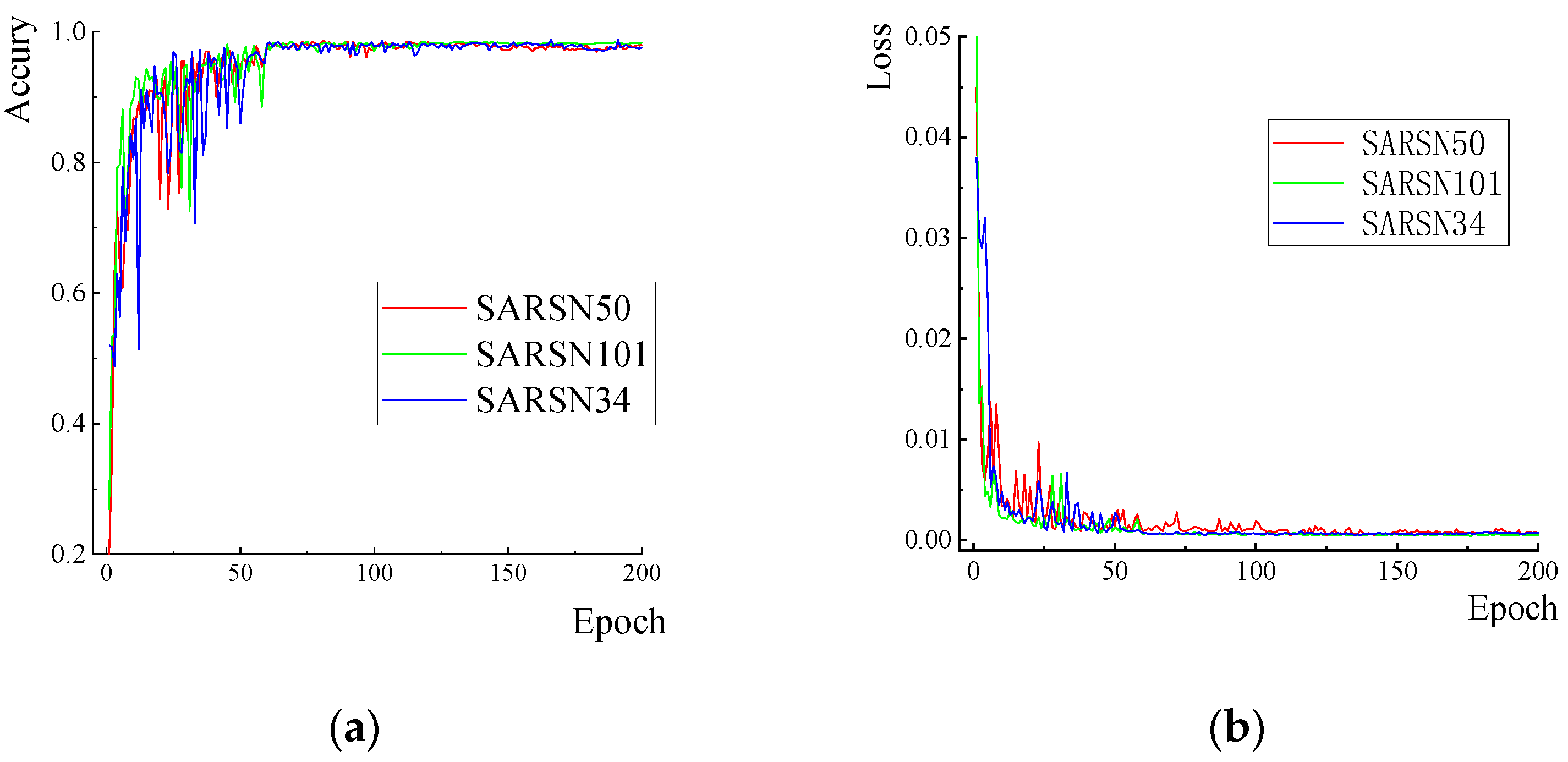
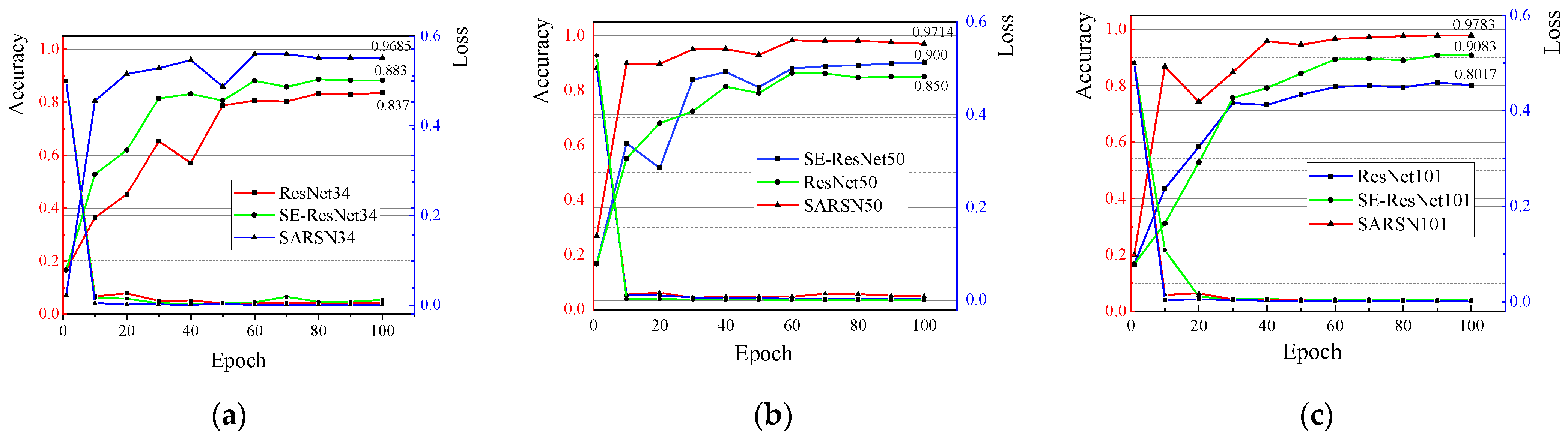
3.2.1. Teacher Model
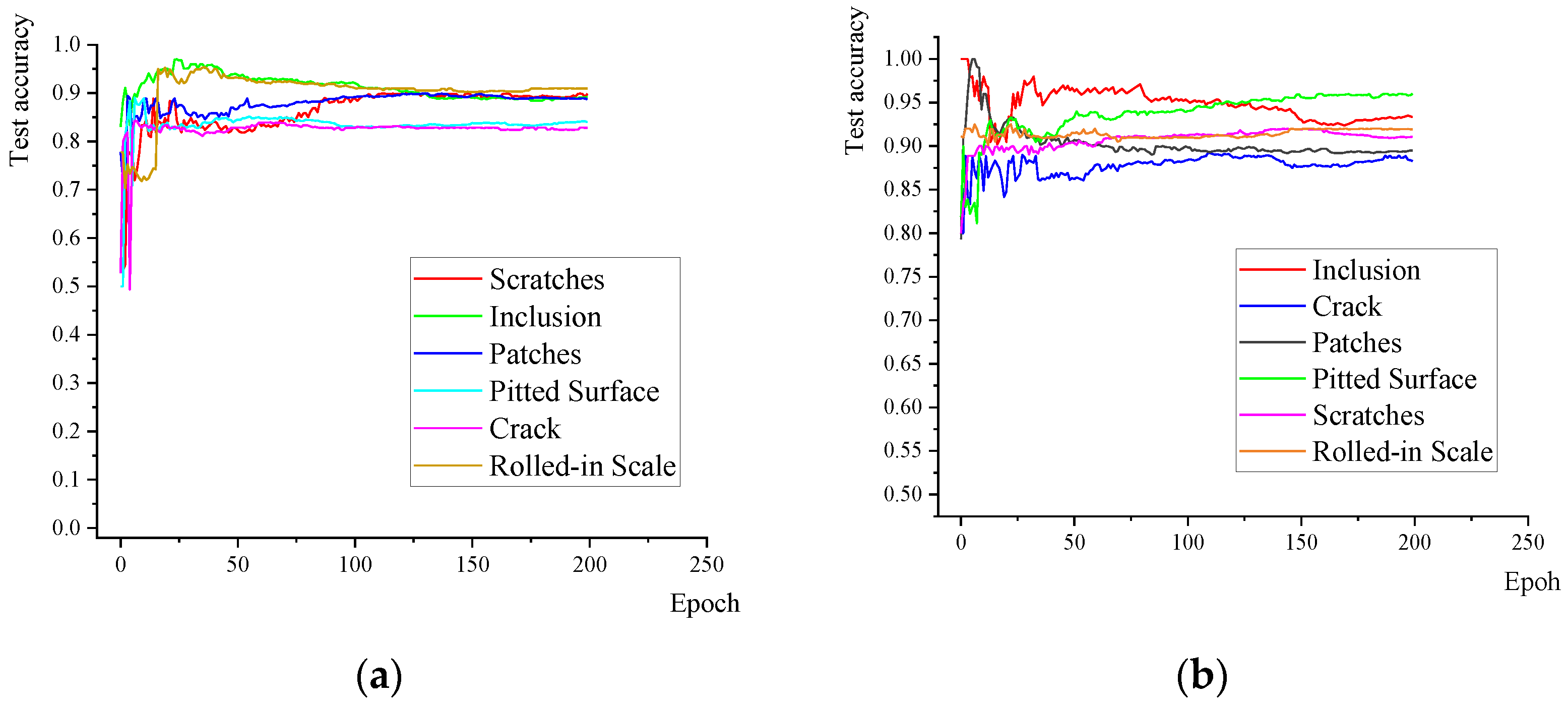
3.2.2. Student Model
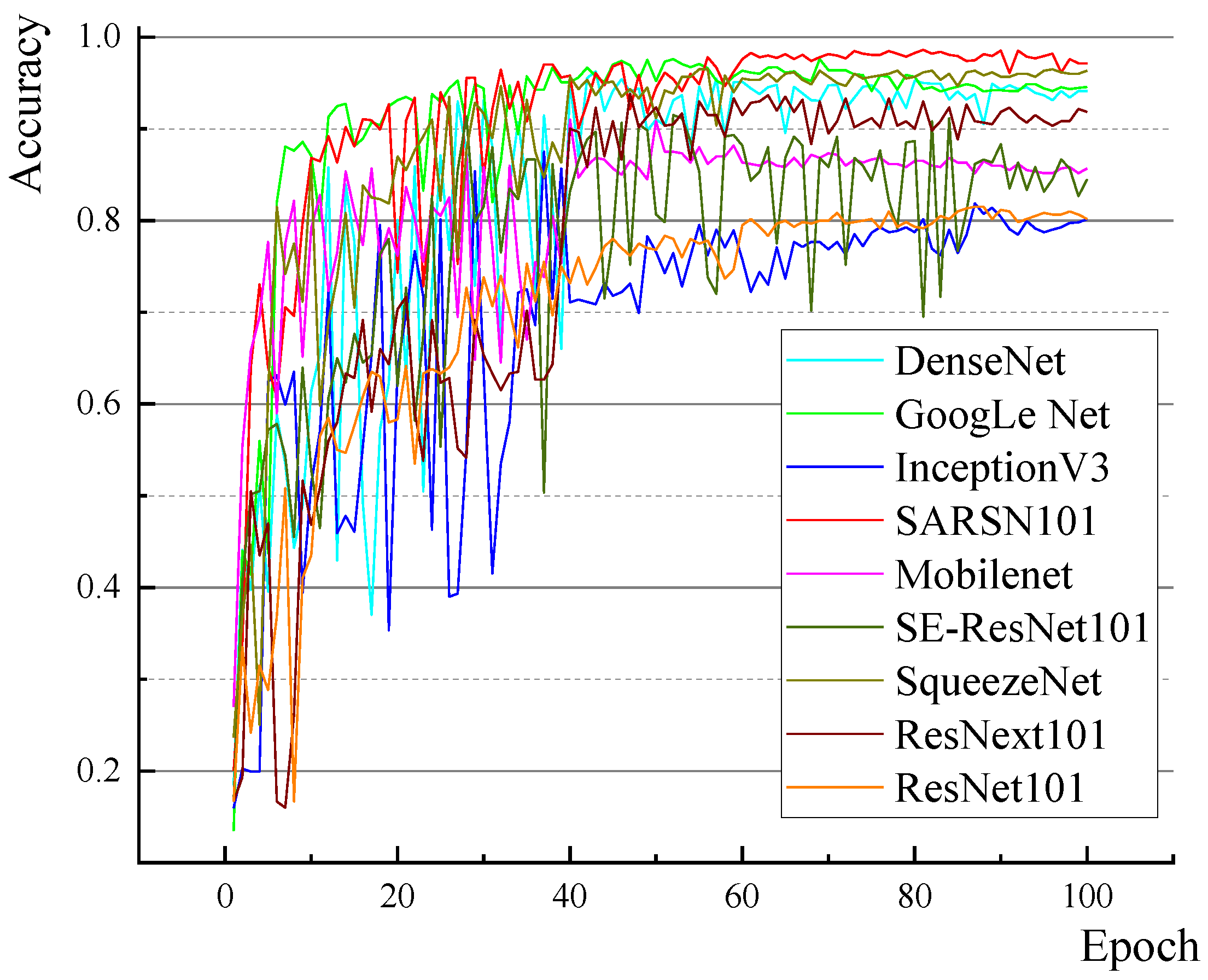
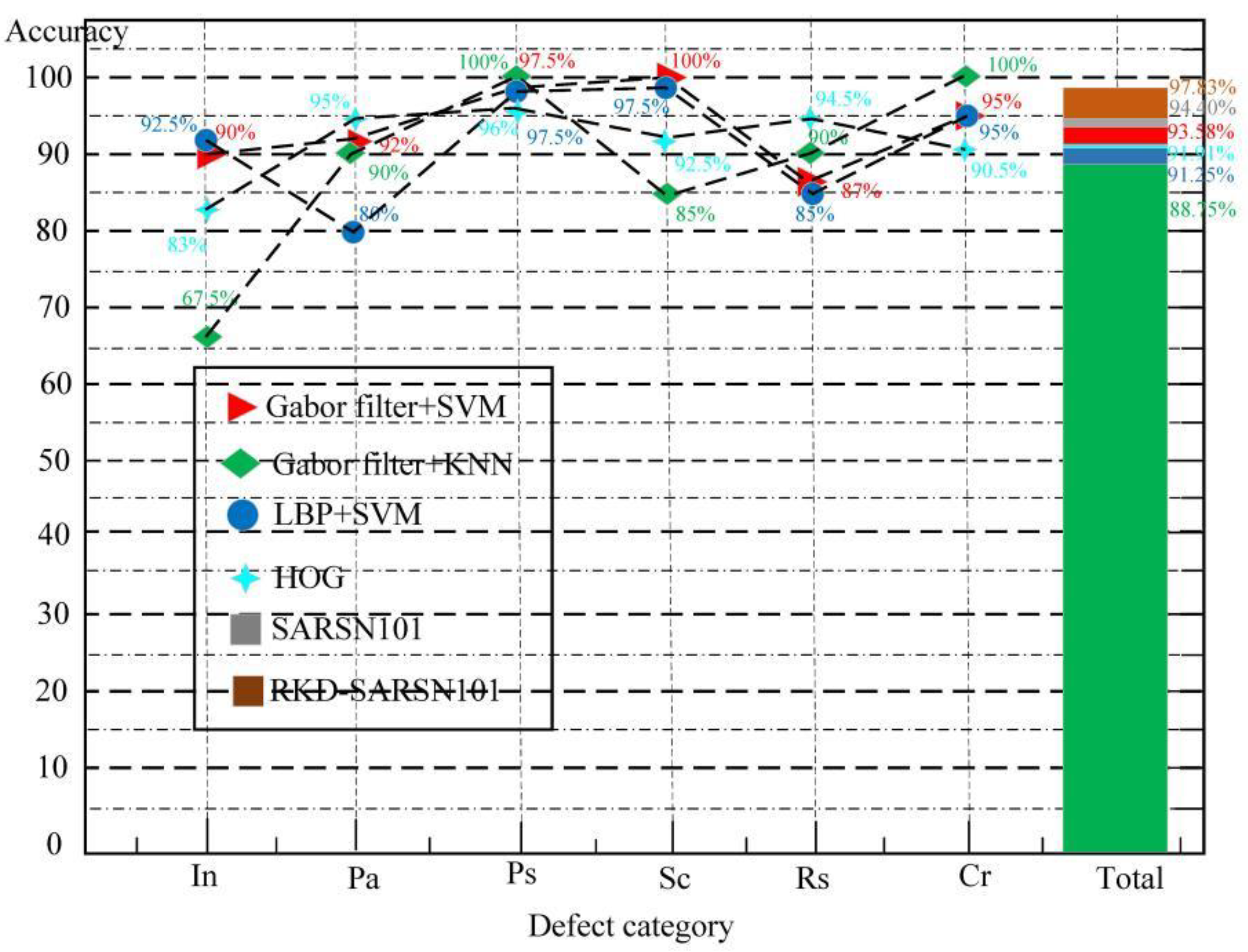
3.2.3. Model Comparative Experiment
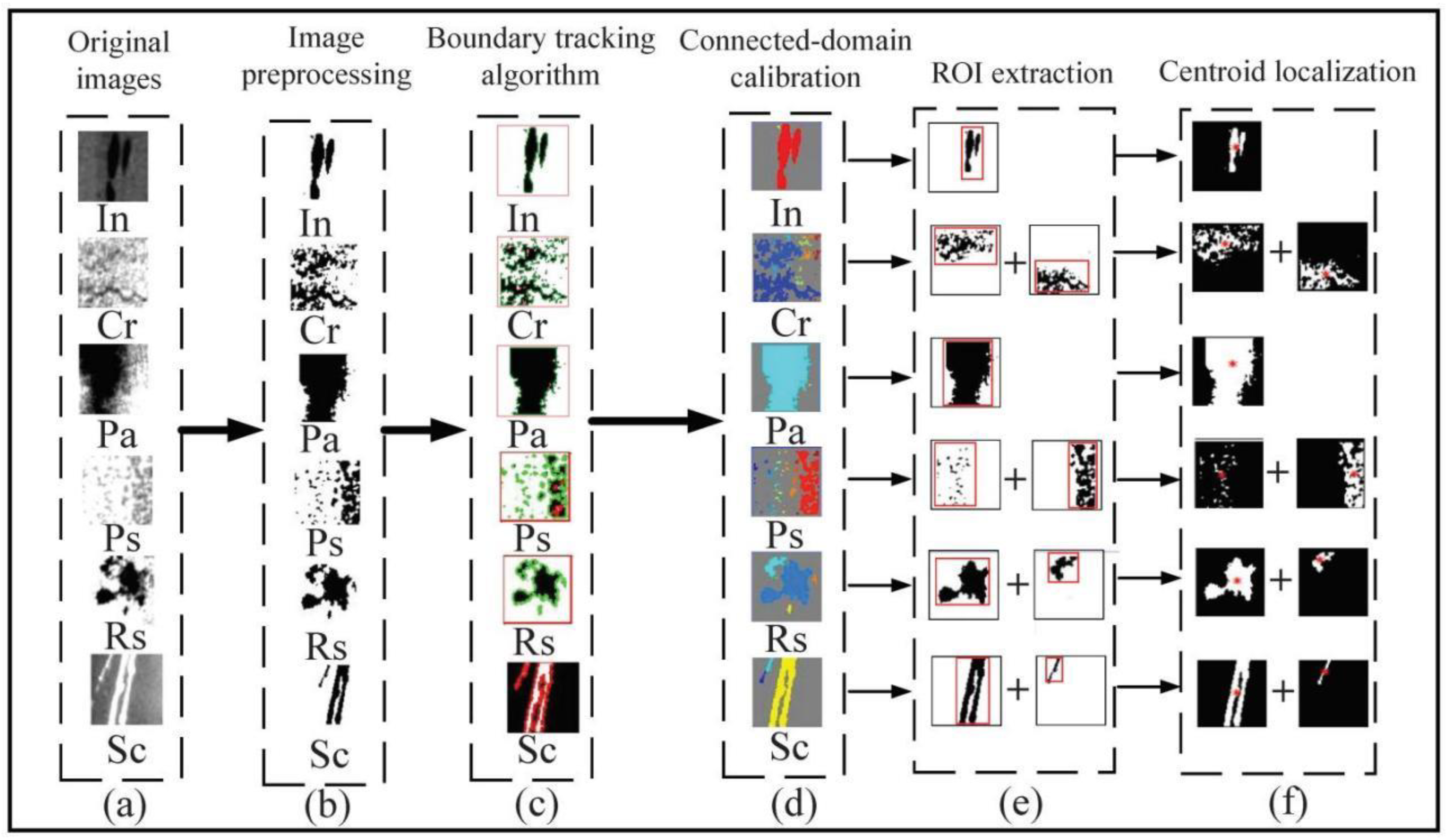
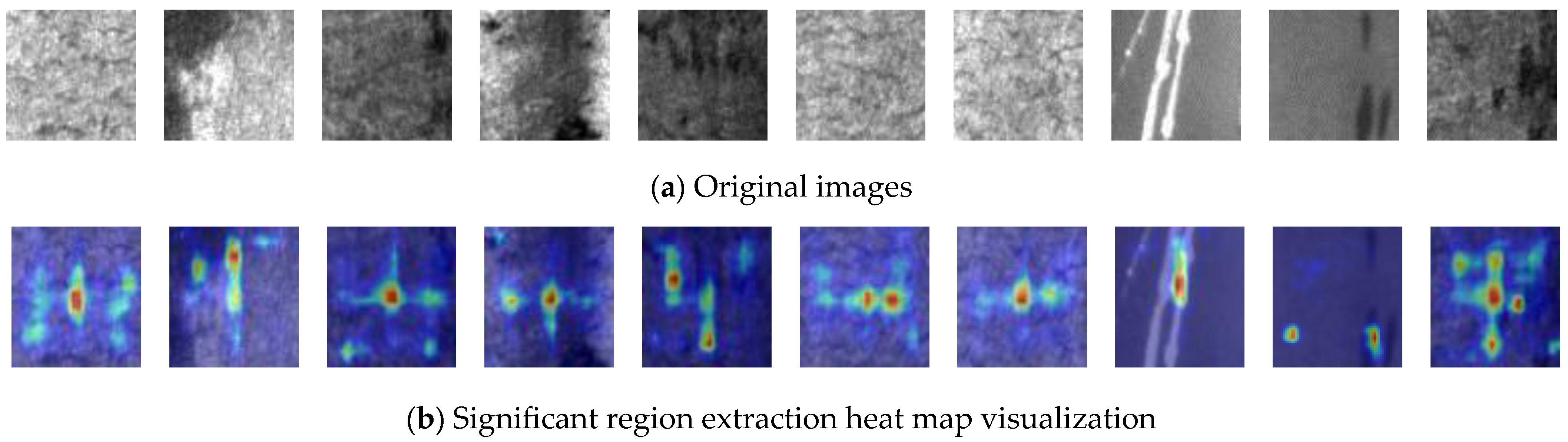
3.2.4. Defect Calculation and Analysis
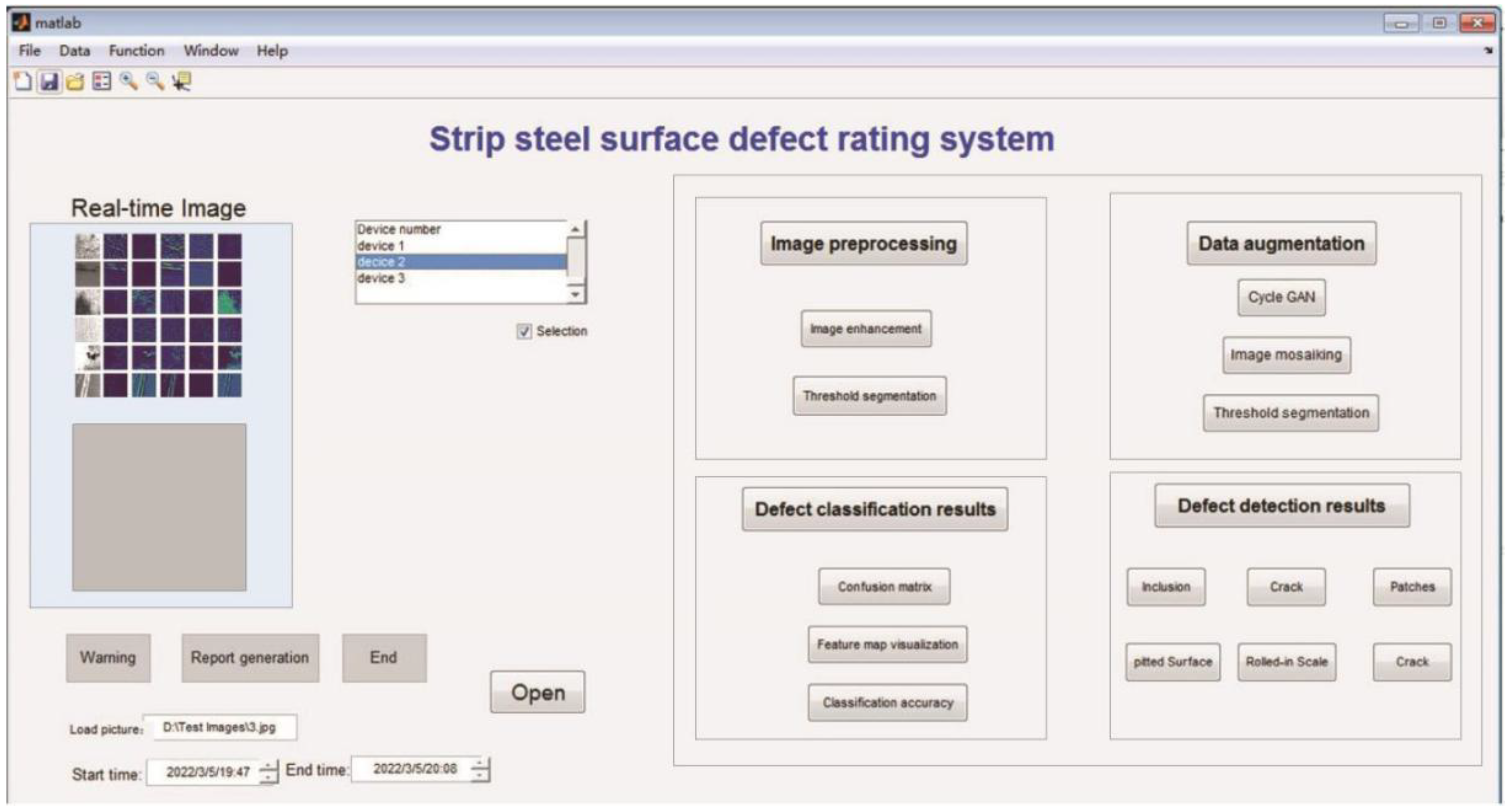
3.2.5. Design of the Grade Evaluation System for Surface Defects of Strip Steel
4. Conclusions
- Using the Cycle GAN data enhancement method can realize cross-domain migration of defective samples of strip steel and solve the problem of few defective samples in a new production line;
- The introduction of the attention mechanism and self-adaptive directional derivative threshold in the SARSN model is the key to improving the classification accuracy of fine-grained defect images;
- In the training process of the model, the self-adaptive loss function balances the differences between classes through a separate class processing mechanism, which is helpful in solving the imbalance problem of strip steel defect samples;
- Structured relational knowledge distillation can transfer the generalization performance of large complex networks to small lightweight networks, reduce the complexity of model calculation and improve the efficiency of model deployment.
- The proposed self-adaptive loss function solves the problem of imbalanced samples between classes, but the sensitivity to highly imbalanced samples is average, and research in this area may need to be strengthened in the future;
- The method of structured relational knowledge distillation is outstanding in improving the detection efficiency of fine-grained image classification tasks, and it is beneficial to deploy it in industrial fields to solve practical problems. However, this method is rarely used in the fault diagnosis of mechanical vibration noise; thus, improving the fault diagnosis efficiency of vibration noise may be a future research direction.
Author Contributions
Funding
Data Availability Statement
Conflicts of Interest
References
- Bhattacharya, G.; Mandal, B.; Puhan, N.B. Interleaved Deep Artifacts-Aware Attention Mechanism for Concrete Structural Defect Classification. IEEE Trans. Image Process. 2021, 30, 6957–6969. [Google Scholar] [CrossRef] [PubMed]
- Dong, X.; Taylor, C.J.; Cootes, T.F. Defect Detection and Classification by Training a Generic Convolutional Neural Network Encoder. IEEE Trans. Signal Process. 2020, 68, 6055–6069. [Google Scholar] [CrossRef]
- Chagas, E.T.C.; Frery, A.C.; Rosso, O.A.; Ramos, H.S. Analysis and Classification of SAR Textures Using Information Theory. IEEE J. Sel. Top. Appl. Earth Obs. Remote Sens. 2021, 14, 663–675. [Google Scholar] [CrossRef]
- Chu, M.X.; Feng, Y.; Yang, Y.H.; Deng, X. Multi-class classification method for steel surface defects with feature noise. J. Iron Steel Res. Int. 2021, 28, 303–315. [Google Scholar] [CrossRef]
- Xu, H.; Yuan, H. An SVM-Based AdaBoost Cascade Classifier for Sonar Image. IEEE Access 2020, 8, 115857–115864. [Google Scholar] [CrossRef]
- Ju, L.; Wang, X.; Zhao, X.; Lu, H.; Mahapatra, D.; Bonnington, P.; Ge, Z. Synergic Adversarial Label Learning for Grading Retinal Diseases via Knowledge Distillation and Multi-task Learning. IEEE J. Biomed. Health Inform. 2021, 25, 3709–3720. [Google Scholar] [CrossRef]
- Guo, N.; Gu, K.; Qiao, J.; Bi, J. Improved deep CNNs based on Nonlinear Hybrid Attention Module for image classification. Neural Netw. 2021, 140, 158–166. [Google Scholar] [CrossRef]
- Chiu, M.-C.; Chen, T.-M. Applying Data Augmentation and Mask R-CNN-Based Instance Segmentation Method for Mixed-Type Wafer Maps Defect Patterns Classification. IEEE Trans. Semicond. Manuf. 2021, 34, 455–463. [Google Scholar] [CrossRef]
- Tu, Z.; Wu, S.; Kang, G.; Lin, J. Real-Time Defect Detection of Track Components: Considering Class Imbalance and Subtle Difference Between Classes. IEEE Trans. Instrum. Meas. 2021, 70, 1–12. [Google Scholar] [CrossRef]
- Jiang, S.; Zhu, Y.; Liu, C.; Song, X.; Li, X.; Min, W. Data set Bias in Few-shot Image Recognition. IEEE Trans. Pattern Anal. Mach. Intell. 2021, 45, 229–246. [Google Scholar] [CrossRef]
- Lv, N.; Ma, H.; Chen, C.; Pei, Q.; Zhou, Y.; Xiao, F.; Li, J. Remote Sensing Data Augmentation Through Adversarial Training. In Proceedings of the IGARSS 2020—2020 IEEE International Geoscience and Remote Sensing Symposium, Brussels, Belgium, 11–16 July 2021; pp. 2511–2514. [Google Scholar]
- Lerner, B.; Yeshaya, J.; Koushnir, L. On the Classification of a Small Imbalanced Cytogenetic Image Database. IEEE ACM Trans. Comput. Biol. Bioinform. 2007, 4, 204–215. [Google Scholar] [CrossRef]
- Jing, X.-Y.; Zhang, X.; Zhu, X.; Wu, F.; You, X.; Gao, Y.; Shan, S.; Yang, J.Y. Multiset Feature Learning for Highly Imbalanced Data Classification. IEEE Trans. Pattern Anal. Mach. Intell. 2021, 43, 139–156. [Google Scholar] [CrossRef] [PubMed]
- Liang, X.; Zhang, Y.; Zhang, J. Attention Multisource Fusion-Based Deep Few-Shot Learning for Hyperspectral Image Classification. IEEE J. Sel. Top. Appl. Earth Obs. Remote Sens. 2021, 14, 8773–8788. [Google Scholar] [CrossRef]
- Li, K.; Wang, X.; Ji, L. Application of Multi-Scale Feature Fusion and Deep Learning in Detection of Steel Strip Surface Defect. In Proceedings of the 2019 International Conference on Artificial Intelligence and Advanced Manufacturing (AIAM), Dublin, Ireland, 16–18 October 2019; pp. 656–661. [Google Scholar]
- Wang, Z.; Wang, J.; Chen, S. Fault Location of Strip Steel Surface Quality Defects on Hot-Rolling Production Line Based on Information Fusion of Historical Cases and Process Data. IEEE Access 2020, 8, 171240–171251. [Google Scholar] [CrossRef]
- Goodfellow, I.J.; Pouget-Abadie, J.; Mirza, M.; Xu, B.; Warde-Farley, D.; Ozair, S.; Courville, A.; Bengio, Y. Generative Adversarial Networks. Adv. Neural Inf. Process. Syst. 2014, 3, 2672–2680. [Google Scholar] [CrossRef]
- Xia, K.; Yin, H.; Qian, P.; Jiang, Y.; Wang, S. Liver Semantic Segmentation Algorithm Based on Improved Deep Adversarial Networks in combination of Weighted Loss Function on Abdominal CT Images. IEEE Access 2019, 7, 96349–96358. [Google Scholar] [CrossRef]
- Creswell, A.; White, T.; Dumoulin, V.; Arulkumaran, K.; Sengupta, B.; Bharath, A.A. Generative Adversarial Networks: An Overview. IEEE Signal Process. Mag. 2018, 35, 53–65. [Google Scholar] [CrossRef]
- He, K.; Zhang, X.; Ren, S.; Sun, J. Deep Residual Learning for Image Recognition. In Proceedings of the 2016 IEEE conference on Computer Vision and Pattern Recognition (CVPR), Las Vegas, NV, USA, 27–30 June 2016; pp. 770–778. [Google Scholar]
- Xie, S.; Girshick, R.; Dollár, P.; Tu, Z.; He, K. Aggregated Residual Transformations for Deep Neural Networks. In Proceedings of the IEEE Conference on Computer Vision and Pattern Recognition (CVPR), Las Vegas, NV, USA, 27–30 June 2016; pp. 1492–1500. [Google Scholar]
- Zhao, M.; Zhong, S.; Fu, X.; Tang, B.; Pecht, M. Deep Residual Shrinkage Networks for Fault Diagnosis. IEEE Trans. Ind. Inform. 2020, 16, 4681–4690. [Google Scholar] [CrossRef]
- Jie, H.; Li, S.; Gang, S.; Albanie, S. Squeeze-and-Excitation Networks. IEEE Trans. Pattern Anal. Mach. Intell. 2017, 42, 2011–2023. [Google Scholar]
- Verma, A.; Sharma, M.; Hebbalaguppe, R.; Hassan, E.; Vig, L. Automatic Container Code Recognition via Spatial Transformer Networks and Connected Component Region Proposals. In Proceedings of the IEEE International Conference on Machine Learning and Applications, Anaheim, CA, USA, 18–20 December 2016; pp. 728–733. [Google Scholar]
- Woo, S.; Park, J.; Lee, J.Y.; Kweon, I.S. CBAM: Convolutional Block Attention Module. In Proceedings of the European Conference on Computer Vision, Munich, Germany, 8–14 September 2018; pp. 3–19. [Google Scholar]
- Sun, C.; Ma, M.; Zhao, Z.; Chen, X. Sparse deep stacking network for fault diagnosis of motor. IEEE Trans. Ind. Inf. 2018, 14, 3261–3270. [Google Scholar] [CrossRef]
- Chen, Y.; Bai, Y.; Zhang, W.; Mei, T. Destruction and Construction Learning for Fine-Grained Image Recognition. In Proceedings of the 2019 IEEE/CVF Conference on Computer Vision and Pattern Recognition (CVPR), Long Beach, CA, USA, 15–20 June 2019; pp. 5157–5166. [Google Scholar]
- Leng, R.; Zhou, W. Optimization Research and Application of Unbalanced Data Set Multi-classification Algorithm. In Proceedings of the International Conference on Intelligent Human-Machine Systems and Cybernetics, Hangzhou, China, 27–28 August 2016; pp. 39–42. [Google Scholar]
- Raj, V.; Magg, S.; Wermter, S. Towards effective classification of imbalanced data with convolutional neural networks. In Proceedings of the IAPR Workshop on Artificial Neural Networks in Pattern Recognition, Ulm, Germany, 28–30 September 2016; pp. 150–162. [Google Scholar]
- Elhanashi, A.; Gasmi, K.; Begni, A.; Dini, P.; Zheng, Q.; Saponara, S. Machine Learning Techniques for Anomaly-Based Detection System on CSE-CIC-IDS2018 Dataset. In Applications in Electronics Pervading Industry, Environment and Society. ApplePies 2022; Berta, R., De Gloria, A., Eds.; Lecture Notes in Electrical Engineering; Springer: Cham, Switzerland, 2023; Volume 1036. [Google Scholar] [CrossRef]
- Anwary, A.R.; Yu, H.; Vassallo, M. Gait Evaluation Using Procrustes and Euclidean Distance Matrix Analysis. IEEE J. Biomed. Health Inform. 2019, 23, 2021–2029. [Google Scholar] [CrossRef] [PubMed]
- Hinton, G.; Vinyals, O.; Dean, J. Distilling the Knowledge in a Neural Network. Comput. Sci. 2015, 14, 38–39. [Google Scholar]
- Park, W.; Kim, D.; Lu, Y.; Cho, M. Relational Knowledge Distillation. In Proceedings of the 2019 IEEE/CVF Conference on Computer Vision and Pattern Recognition (CVPR), Long Beach, CA, USA, 15–20 June 2019; pp. 3967–3976. [Google Scholar]
- Angelopoulos, A.; Michailidis, E.T.; Nomikos, N.; Trakadas, P.; Hatziefremidis, A.; Voliotis, S.; Zahariadis, T. Tackling faults in the industry 4.0 era—A survey of machine-learning solutions and key aspects. Sensors 2019, 20, 109. [Google Scholar] [CrossRef] [PubMed]
- Hao, R.; Lu, B.; Cheng, Y.; Li, X.; Huang, B. A steel surface defect inspection approach towards smart industrial monitoring. J. Intell. Manuf. 2021, 32, 1833–1843. [Google Scholar] [CrossRef]
- Tang, B.; Chen, L.; Sun, W.; Lin, Z.K. Review of surface defect detection of steel products based on machine vision. IET Image Process. 2023, 17, 303–322. [Google Scholar] [CrossRef]
- Czimmermann, T.; Ciuti, G.; Milazzo, M.; Chiurazzi, M.; Roccella, S.; Oddo, C.M.; Dario, P. Visual-based defect detection and classification approaches for industrial applications—A survey. Sensors 2020, 20, 1459. [Google Scholar] [CrossRef]
- Sampath, V.; Maurtua, I.; Martín, J.J.A.; Rivera, A.; Molina, J.; Gutierrez, A. Attention guided multi-task learning for surface defect identification. IEEE Trans. Ind. Inform. 2023, 19, 9713–9721. [Google Scholar] [CrossRef]
- Nnolim, U.A. Multi-Scale Fractional Tonal Correction Bilateral Filter-Based Hazy Image Enhancement. Int. J. Image Graph. 2020, 20, 2050010. [Google Scholar] [CrossRef]
- Tian, F.; Gao, Y.; Fang, Z.; Gu, J. Automatic coronary artery segmentation algorithm based on deep learning and digital image processing. Appl. Intell. 2021, 51, 8881–8895. [Google Scholar] [CrossRef]


| In | Cr | Pa | Ps | Rs | Sc | |
|---|---|---|---|---|---|---|
| Original drawing |  |  |  |  |  |  |
| Image enhancement |  |  |  |  |  |  |
| Threshold segmentation |  |  |  |  |  |  |
| Defect calibration |  |  |  |  |  |  |
| Comparison of Cycle GAN Defect Sample before and after Migration | ||||
|---|---|---|---|---|
| Sc original |  |  |  |  |
| Sc generation |  |  |  |  |
| In original |  |  |  |  |
| In generation |  |  |  |  |
| Rs original |  |  |  |  |
| Rs generation |  |  |  |  |
| Teacher Mode | Training Accuracy | Testing Accuracy |
|---|---|---|
| SARSN34 | 97.80% | 96.85% |
| SARSN50 | 98.27% | 97.14% |
| SARSN101 | 98.33% | 97.83% |
| Teacher Mode | Student Model | Training Accuracy |
|---|---|---|
| SARSN34 | ResNet34 | 90.56% |
| SARSN50 | ResNet34 | 92.31% |
| SARSN101 | ResNet34 | 95.23% |
| ______ | ResNet34 | 89.18% |
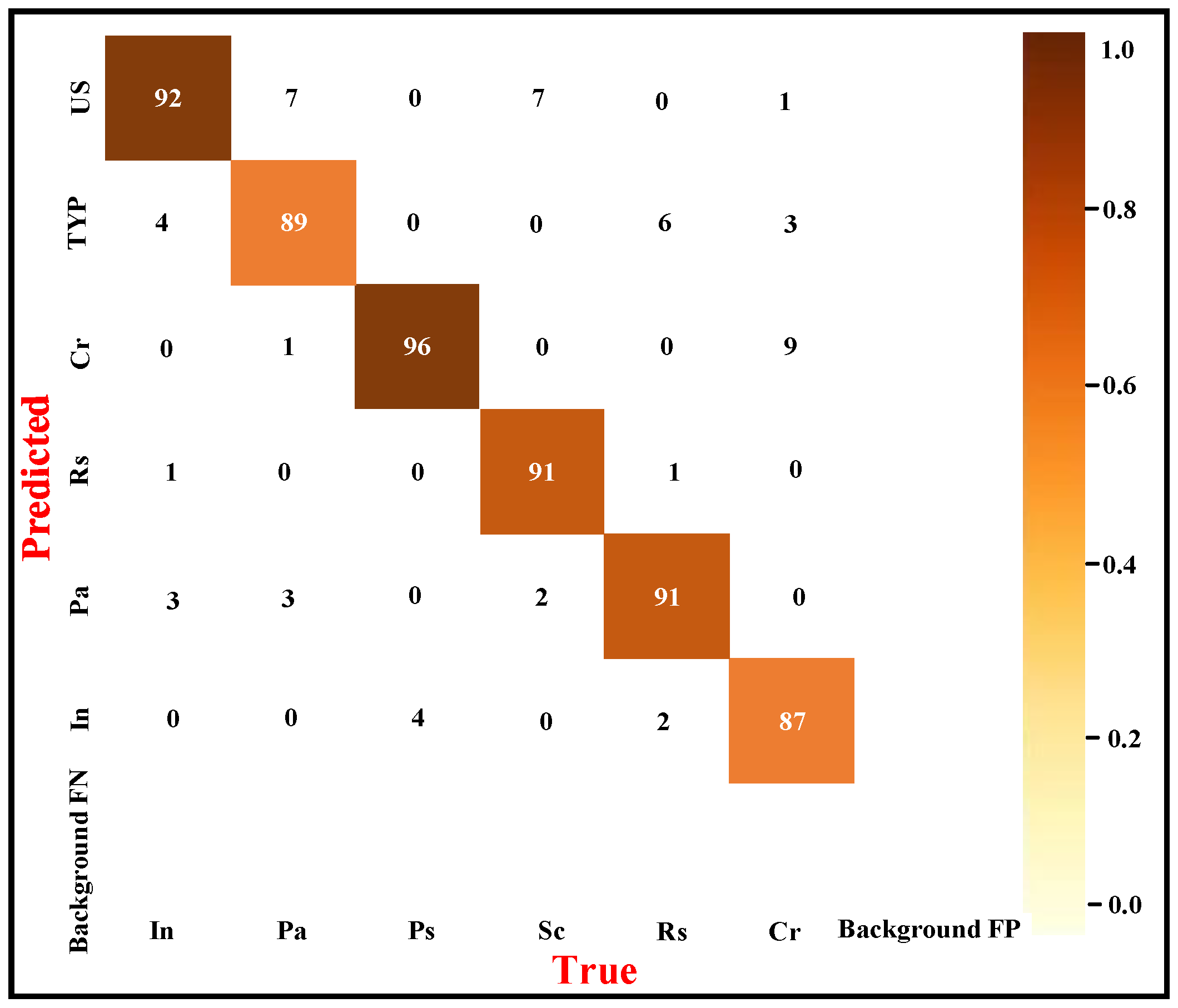
| Defect Category | P | R | F1 |
|---|---|---|---|
| In | 0.860 | 0.920 | 0.890 |
| Pa | 0.873 | 0.890 | 0.881 |
| Ps | 0.906 | 0.960 | 0.932 |
| Sc | 0.978 | 0.910 | 0.943 |
| Rs | 0.919 | 0.910 | 0.915 |
| Cr | 0.935 | 0.870 | 0.901 |
| Model | Test Accuracy | Parameter Number | Time-Consumption/(ms) |
|---|---|---|---|
| GoogLeNet | 0.9407 | 6,306,214 | 58 |
| DenseNet | 0.9413 | 6,952,198 | 96 |
| InceptionV3 | 0.8011 | 22,125,542 | 248 |
| SqueezeNet | 0.9633 | 732,934 | 104 |
| MobileNetV2 | 0.8567 | 3,219,078 | 7.8 |
| ResNet101 | 0.8017 | 42,504,774 | 112 |
| ResNext101 | 0.9167 | 14,788,772 | 67 |
| SE-ResNet101 | 0.8451 | 47,527,764 | 187 |
| SARSN101 | 0.9783 | 46,127,174 | 85 |
| Teacher-SARSN101 Student-ResNet34 | 0.9440 | 11,171,910 | 51 |
| Category | Area (Point) | Perimeter (Point) | Area Ratio (%) | Perimeter-Area Ratio (K) |
|---|---|---|---|---|
| Cr | 1.646 × 10³ | 475.911 | 40.18% | 0.289 |
| In | 0.759 × 10³ | 71.414 | 18.53% | 0.094 |
| Pa | 2.332 × 10³ | 113.314 | 56.93% | 0.048 |
| Ps | 1.019 × 10³ | 368.426 | 24.88% | 0.362 |
| Rs | 1.159 × 10³ | 213.012 | 28.30% | 0.183 |
| Sc | 0.789 × 10³ | 82.243 | 19.48% | 0.103 |
Disclaimer/Publisher’s Note: The statements, opinions and data contained in all publications are solely those of the individual author(s) and contributor(s) and not of MDPI and/or the editor(s). MDPI and/or the editor(s) disclaim responsibility for any injury to people or property resulting from any ideas, methods, instructions or products referred to in the content. |
© 2023 by the authors. Licensee MDPI, Basel, Switzerland. This article is an open access article distributed under the terms and conditions of the Creative Commons Attribution (CC BY) license (https://creativecommons.org/licenses/by/4.0/).
Share and Cite
Huang, X.; Song, Z.; Ji, C.; Zhang, Y.; Yang, L. Research on a Classification Method for Strip Steel Surface Defects Based on Knowledge Distillation and a Self-Adaptive Residual Shrinkage Network. Algorithms 2023, 16, 516. https://doi.org/10.3390/a16110516
Huang X, Song Z, Ji C, Zhang Y, Yang L. Research on a Classification Method for Strip Steel Surface Defects Based on Knowledge Distillation and a Self-Adaptive Residual Shrinkage Network. Algorithms. 2023; 16(11):516. https://doi.org/10.3390/a16110516
Chicago/Turabian StyleHuang, Xinbo, Zhiwei Song, Chao Ji, Ye Zhang, and Luya Yang. 2023. "Research on a Classification Method for Strip Steel Surface Defects Based on Knowledge Distillation and a Self-Adaptive Residual Shrinkage Network" Algorithms 16, no. 11: 516. https://doi.org/10.3390/a16110516
APA StyleHuang, X., Song, Z., Ji, C., Zhang, Y., & Yang, L. (2023). Research on a Classification Method for Strip Steel Surface Defects Based on Knowledge Distillation and a Self-Adaptive Residual Shrinkage Network. Algorithms, 16(11), 516. https://doi.org/10.3390/a16110516