Trustworthy Digital Representations of Analog Information—An Application-Guided Analysis of a Fundamental Theoretical Problem in Digital Twinning ^†

Abstract

This article compares two methods of algorithmically processing bandlimited time-continuous signals in light of the general problem of finding “suitable” representations of analog information on digital hardware. Albeit abstract, we argue that this problem is fundamental in digital twinning, a signal-processing paradigm the upcoming 6G communication-technology standard relies on heavily. Using computable analysis, we formalize a general framework of machine-readable descriptions for representing analytic objects on Turing machines. Subsequently, we apply this framework to sampling and interpolation theory, providing a thoroughly formalized method for digitally processing the information carried by bandlimited analog signals. We investigate discrete-time descriptions, which form the implicit quasi-standard in digital signal processing, and establish continuous-time descriptions that take the signal’s continuous-time behavior into account. Motivated by an exemplary application of digital twinning, we analyze a textbook model of digital communication systems accordingly. We show that technologically fundamental properties, such as a signal’s (Banach-space) norm, can be computed from continuous-time, but not from discrete-time descriptions of the signal. Given the high trustworthiness requirements within 6G, e.g., employed software must satisfy assessment criteria in a provable manner, we conclude that the problem of “trustworthy” digital representations of analog information is indeed essential to near-future information technology.

1. Introduction

State-of-the-art technological information processing happens mainly within the digital realm. Numerical values are quantized, and calculations are performed in discrete-time computational cycles. In contrast, the information carried by the physical world surrounding any technological device is analog and continuous. Twelve years after Alan Turing formalized the notion of digital computing [1], Claude Shannon established the theoretical foundation of sampling and interpolation theory [2]. Since then, scientists and engineers have extended Turing’s and Shannon’s theories and refined the relevant hardware, making the analog world increasingly accessible to digital information processing.

As follows from Shannon’s sampling theorem, suitable (infinite) interpolation series uniquely restore any bandlimited continuous-time signal, provided that the signal’s energy is finite and the samples are taken at least at the Nyquist rate. In its purest form, this result is present in signal processing and communications technology in the context of analog–digital/digital–analog conversion. In principle, however, any computational discretization method, such as finite-element algorithms, employs a similar paradigm: A set of discrete points, sufficiently dense for the in-between to become negligible, represents some continuous, physical object (c.f. [3] for a recent example in which the physical “object” is an electromagnetic field).

Another recent concept in the domain of digital information processing is known as digital twinning. According to the formalization established in [4], digital twinning commonly involves a physical entity to be twinned, a machine-readable description (in some machine-readable language) that represents the entity virtually on an appropriate hardware platform, and an interaction between the entity and its description through measurement and control. In this context, the machine-readable description is the entity’s digital twin. More generally, if the particular type of computing hardware is not specified, we refer to the entity’s virtual representation as a virtual twin. Furthermore, the term “entity” indicates that the virtual twin’s physical counterpart does not necessarily have to be an actual object. In theory, any abstract formation—such as, for example, an entire communication network [5], or, as above, an electromagnetic field—qualifies for digital twinning, provided we can characterize it by a suitable mathematical model. Despite the different contexts, digital twinning resembles traditional Shannon Sampling and Interpolation (SSI) in some aspects. Both approaches represent a physical entity (in the context of SSI, a bandlimited signal) using digital data, digitalizing the relevant analog information through a sequential measurement process. However, classical SSI is geared towards completely restoring the physical entity, while digital twinning primarily aims to recover the entity’s relevant properties. Within the employed mathematical model, relevant properties usually take the form of a (mathematical) function or relation with a particular interpretation on the practical level, such as the position of a material object at a given time or the total energy contained in an electromagnetic field.

Originally associated primarily with Industry 4.0 [6], digital twinning is attracting significant interest in many areas of modern technology. As part of the internet’s anticipated evolution towards a unified metaverse, even more facets of the physical environment will connect to virtual space. In particular, information processing will increasingly incorporate the interaction between human multi-modalities (human senses) and the digital domain, c.f. [7]. In order to make human senses experienceable, the computational infrastructure will have to coordinate, process, and distribute the relevant information in real time. This requirement imposes engineers with unprecedented technological challenges regarding optimization, control, and decision-making. In this regard, research and development advocates digital twinning as one of several critical enablers. The novel technological applications that researchers envision in the context of digital twinning are just as ambitious. Medical research, for example, considers applications such as disease-trajectory estimation, optimization of medical-care timing, identification of biomarkers or elucidation of drug mechanisms, and patient-tailored prediction of treatment effects, employing digital twins of, e.g., a patient’s immune system [8].

Given the potential for hazardous impacts of future digital-twinning applications on sensitive aspects of human well-being, the need to follow strict specifications on privacy, integrity, reliability, and safety is manifest. The upcoming 6G industry standard for communication technologies, which incorporates large parts of the technological infrastructure for the metaverse and other digital-twinning applications, summarizes such requirements by the term trustworthiness [9]. Depending on the potential hazards of an application, the physical entity’s relevant properties must be reliably recoverable from the entity’s digital twin. In practice, technological systems for critical applications must undergo technology assessment, which evaluates the implementation with regard to criteria of provable performance. When expressed in mathematical terms, e.g., by a margin of error, the recovered property must almost surely meet, such criteria entail “sufficient” and “insufficient” ways of representing a physical entity in virtual space. That is, the employed machine-readable language must satisfy specific structural characteristics, such that the relevant properties can be reliably computed from any of the entity’s machine-readable descriptions. We summarize this observation in terms of the following fundamental problem statement, which we aim to elaborate on throughout this article.

Given an application that requires the processing of analog information, find a sufficient way to represent the information on the chosen hardware platform.

The problem statement refers to general hardware platforms. As previously indicated, future virtual-twinning applications will not necessarily be limited to digital technology, c.f. [4]. However, in the scope of this article, we will only discuss traditional digital computing. Hence, in the problem statement, we may replace “the chosen hardware platform” with “digital hardware” in the context of the subsequent sections.

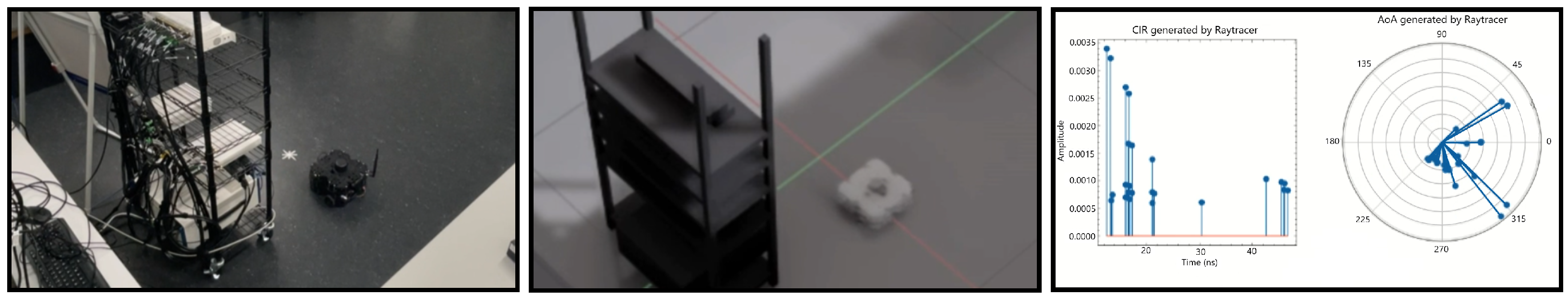
So far, our discussion on the fundamental problem statement and the associated concepts has been abstract, without a clear picture of how they translate to actual engineering problems. Throughout the subsequent sections, we aim to draw a precise picture of machine-readable languages, relevant properties, and proper representations for signal-processing and communications-engineering applications that involve traditional SSI. Aside from the conceptual similarities between digital twinning and SSI we discussed above, SSI has relevant direct applications in digital twinning. In the context of general virtual twinning, ref. [10] discussed an actual implementation of such an application, c.f. Figure 1.

Figure 1. Application of digital twinning as discussed in [10]. (Left) A robot (physical entity) is moving on the floor of a laboratory environment. It is sequentially measuring its position relative to a fixed coordinate system and transmitting the relevant data through wireless communication to a receiving end. (Middle) The receiving end tracks the position and forms a virtual representation (digital twin) of the robot inside the room. It updates the virtual representation to match the physical robot whenever new information becomes available. The depicted image is thus a visualization of the robot’s instantaneous machine-readable description. (Right) Using the robot’s virtual representation, the receiving end computes the impulse response of the wireless communication link (the depicted implementation uses a ray-tracing approach), i.e., a sequence of samples representing a bandlimited signal. In essence, the impulse response forms a digital twin of the communication link.

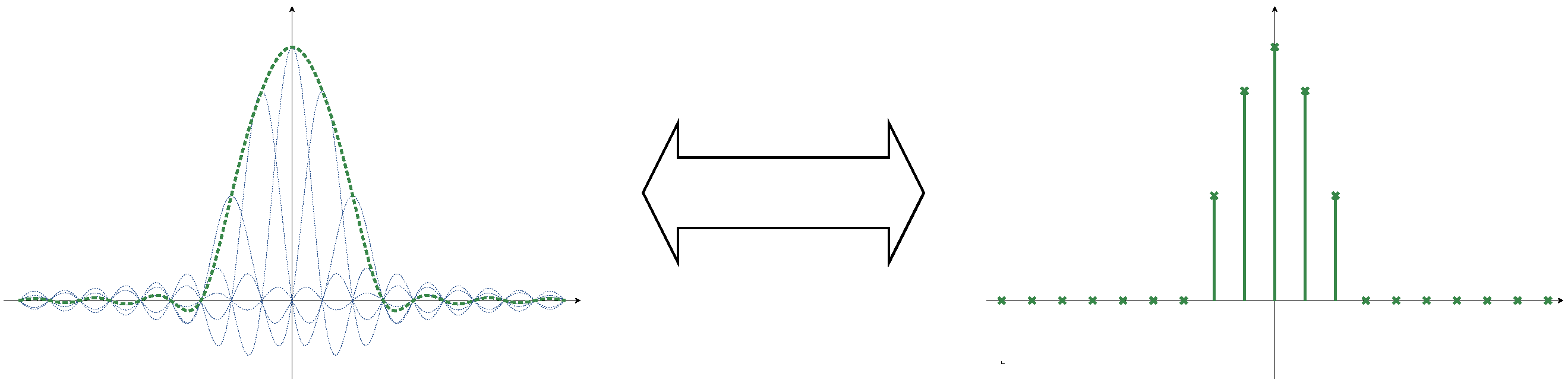
Recall that traditional SSI aims at restoring the physical entity (i.e., a bandlimited signal) entirely. The relevant analytic result is known as (generalized) Plancherel–Pólya Theorem, c.f. Section 2 and Figure 2: The bandlimited signal uniquely determines the corresponding sequence of samples, and vice versa.

Figure 2. Generalized Plancherel–Pólya Theorem (c.f. Section 2). By evaluating a bandlimited, continuous-time signal (left) at all integer multiples of a suitable sampling interval T, we obtain the sequence of samples (right) corresponding to the function under consideration. We can restore the function through an (infinite) interpolation series, where each term is associated with one of the sample sequence’s components. In particular, each term consists of a time-shifted interpolation function multiplied by the associated sample. This way, the bandlimited function and the sequence of sampling values uniquely determine each other.

Accordingly, we expect that any property of the bandlimited signal should be recoverable from the sequence of sampling values. At this point, Turing’s theory of digital computing enters the stage: A priori, the (generalized) Plancherel–Pólya Theorem is a purely analytic result. For it to hold on the algorithmic level, effectiveness in the sense of computable analysis is required. In this context, we will analyze two machine-readable languages emerging from the (generalized) Plancherel–Pólya Theorem for their structural properties. We employ the theory of Turing machines and effective analysis, classifying our results in terms of digital twinning and the article’s fundamental problem statement. Particularly, we provide formal definitions of the terms machine-readable languages and machine-readable descriptions, and discuss formal examples of relevant properties. After the mathematical part of the article, we provide a brief subsumption and interpretation of our results, together with some prospects of how they affect near-future digital information-processing technology.

The remainder of the article is structured as follows. In Section 2, we provide some mathematical background on SSI, introducing the signal spaces ${\mathcal{l}}_0^{\infty }, {\mathcal{l}}_0^1,{\mathcal{B}}_{0,\pi }^{\infty },$ and ${\mathcal{B}}_{\pi }^1$, and formally establishing the (generalized) Plancherel–Pólya Theorem in terms of the Banach-space operators ${\mathit{S}}_{★}:\mathcal{B}(★)\to \mathcal{l}(★)$ and ${\mathit{T}}_{★}:={\mathit{S}}_{★}^{-1}$. Applying the theory of Turing computability and effective analysis, we continue to develop a framework of machine-readable languages for ${\mathcal{B}}_{0,\pi }^{\infty }$ and ${\mathcal{B}}_{\pi }^1$. This framework formalizes the traditional theory of digital signal processing for communications engineering based on a mathematically rigorous notion of computability. Particularly, we define the machine-readable languages ${\mathfrak{X}}_1$ and ${\mathfrak{X}}_{\infty }$, which mirror the implicit quasi-standard in digital signal processing, and the machine-readable languages ${\mathfrak{F}}_1$ and ${\mathfrak{F}}_{\infty }$, which take the relevant signal’s continuous-time behavior into account. In Section 3, we provide (for didactic purposes) a mathematical model of digital-twinning systems such as the one shown in Figure 1, marking the Banach-space norms ${\parallel ·\parallel }_{\infty }$ and ${\parallel ·\parallel }_1$ as a relevant property of signals $\mathit{f}\in {\mathcal{B}}_{0,\pi }^{\infty }$, $\mathit{f}\in {\mathcal{B}}_{\pi }^1$, respectively. Guided by the exemplary application case, we establish our main results: The (generalized) Plancherel–Pólya Theorem does not hold true on the algorithmic level. Depending on which of the established machine-readable languages we choose, we either can or cannot compute ${\parallel \mathit{f}\parallel }_{\infty }$, ${\parallel \mathit{f}\parallel }_1$, respectively, despite all languages determining the relevant signals uniquely in the (analytic) sense of the (generalized) Plancherel–Pólya Theorem. Finally, Section 4 discusses several other signal properties our theory can analyze and closes the article by interpreting our results as indicated above.

2. Materials and Methods

In the following, we provide a concise introduction to the mathematics of sampling and interpolation, which are primarily based on the theory of Banach spaces and linear operators. To this end, we introduce the Banach spaces ${\mathcal{l}}_0^{\infty },{\mathcal{l}}^p,{\mathcal{B}}_{0,\sigma }^{\infty },$ and ${\mathcal{B}}_{\sigma }^p$, $1\le p<\infty$, $0<\sigma <\infty$. Commonly, ${\mathcal{B}}_{0,\sigma }^{\infty }$ and ${\mathcal{B}}_{\sigma }^p$ are referred to as Bernstein spaces. For a comprehensive introduction, we refer the reader to [11,12].

By ${\mathcal{l}}_0^{\infty }$, we denote the set of all complex-valued sequences indexed by $\mathbb{Z}$ that vanish at infinity. That is, we have

$$\begin{array}{c}\hfill \underset{k\to \infty }{lim}\mathit{x}\left[k\right]=\underset{k\to -\infty }{lim}\mathit{x}\left[k\right]=0\end{array}$$

for all $\mathit{x}={\left(\mathit{x}\left[k\right]\right)}_{k\in \mathbb{Z}}\in {\mathcal{l}}_0^{\infty }$. Equipped with the uniform norm ${\parallel \mathit{x}\parallel }_{\infty }:={sup}_{k\in \mathbb{Z}}\left|\mathit{x}\left[k\right]\right|$ the set ${\mathcal{l}}_0^{\infty }$ becomes a Banach space. Further, by ${\mathcal{l}}^p$, $1\le p<\infty$, we denote the Banach space of pth-power-summable sequences with the p-norm

$$\begin{array}{c}\hfill {\parallel \mathit{x}\parallel }_p:={\left(\sum _{k=-\infty }^{\infty }{\left|\mathit{x}\left[k\right]\right|}^p\right)}^{1/p}.\end{array}$$

A function $\mathit{f}:\mathbb{C}\to \mathbb{C},z\mapsto \mathit{f}\left(z\right)$ is called entire if it is well-defined and holomorphic on all of $\mathbb{C}$. For entire functions that are (essentially) bounded on the real line, we define the essential-supremum norm ${\parallel \mathit{f}\parallel }_{\infty }:={ess\; sup}_{t\in \mathbb{R}}\left|\mathit{f}\left(t\right)\right|$. The space ${\mathcal{B}}_{0,\sigma }^{\infty }, 0<\sigma <\infty ,$ consists of all entire functions $\mathit{f}$ that satisfy the following conditions:

• $\mathit{f}$ is (essentially) bounded on the real line;
• $\mathit{f}$ of exponential type (c.f. [11], Lecture 1, p. 3ff) at most $\sigma$;
• $\mathit{f}\left(t\right)$ vanishes for $t\to \pm \infty$ on the real line.

Equipped with the essential supremum norm, the space ${\mathcal{B}}_{0,\sigma }^{\infty }$ becomes a Banach space. Further, the Banach spaces ${\mathcal{B}}_{\sigma }^p$, $1\le p<\infty$, consists of all functions in ${\mathcal{B}}_{0,\sigma }^{\infty }$ that are pth-power integrable on the real line, equipped with the p-norm

$$\begin{array}{c}\hfill {\parallel \mathit{f}\parallel }_p:={\left({\int }_{t\in \mathbb{R}}{\left|\mathit{f}\left(t\right)\right|}^p\mathrm{d}t\right)}^{1/p}.\end{array}$$

Pure mathematics studies all of the spaces ${\mathcal{l}}_0^{\infty },{\mathcal{l}}^p,{\mathcal{B}}_{0,\sigma }^{\infty },$ and ${\mathcal{B}}_{\sigma }^p$, $1\le p<\infty$, $0<\sigma <\infty$. In contrast, only the spaces ${\mathcal{l}}^1,{\mathcal{l}}^2,{\mathcal{l}}_0^{\infty }$ and ${\mathcal{B}}_{\sigma }^1,{\mathcal{B}}_{\sigma }^2,{\mathcal{B}}_{0,\sigma }^{\infty }$ occur frequently throughout signal processing and communications engineering, the arguably most “well-known” ones being ${\mathcal{l}}^2$ and ${\mathcal{B}}_{\sigma }^2$. They consist of discrete- and, respectively, bandlimited continuous-time signals with finite energy and form the mathematical basis for the seminal results in SSI, established before the relevant theory was extended to general Bernstein spaces. Fourier analysis provides a bijective isometry between ${\mathcal{l}}^2$ and ${\mathcal{B}}_{\sigma }^2$: defining ${\mathit{x}}_{\mathit{f}}\left[k\right]:=\mathit{f}(k\pi /\sigma ),k\in \mathbb{Z}$, we have

$$\begin{array}{cc}\hfill \left[\widetilde{\mathcal{F}\mathit{f}}\right]\left(\xi \right):& =\sqrt{\frac{\pi }{2{\sigma }^2}}\sum _{k=-\infty }^{\infty }{\mathit{x}}_{\mathit{f}}\left[k\right]{\mathrm{e}}^{-j\pi k\xi /\sigma },\hfill \\ \hfill \left[\mathcal{F}\mathit{f}\right]\left(\xi \right):& =\frac{1}{\sqrt{2\pi }}{\int }_{t\in \mathbb{R}}\mathit{f}\left(t\right){\mathrm{e}}^{-j\xi t}\mathrm{d}t=\left\{\begin{array}{cc}\left[\widetilde{\mathcal{F}\mathit{f}}\right]\left(\xi \right),\hfill & \mathrm{if}-\sigma \le \xi \le \sigma ,\hfill \\ 0,\hfill & \mathrm{otherwise},\hfill \end{array}\right.\hfill \end{array}$$

for all $\mathit{f}\in {\mathcal{B}}_{\sigma }^2$, where $\mathcal{F}\mathit{f}$ denotes the Fourier Transform of $\mathit{f}$ on the real line. Through the definition of the sinc-function,

$$\begin{array}{c}\hfill sinc\left(z\right):=\left\{\begin{array}{cc}\frac{sin\left(\pi z\right)}{\pi z}\hfill & \mathrm{if} z\ne 0,\hfill \\ 1\hfill & \mathrm{if} z=0,\hfill \end{array}\right.,z\in \mathbb{C},\end{array}$$

and the linearity of the Fourier Transform, the isometry provides Shannon’s original sampling theorem for the spaces ${\mathcal{l}}^2$ and ${\mathcal{B}}_{\sigma }^2$, we have

$$\begin{array}{c}\hfill \underset{N\to \infty }{lim}{\int }_{\mathbb{R}}{\left|\mathit{f}\left(t\right)-\sum _{k=-N}^N{\mathit{x}}_{\mathit{f}}\left[k\right]sinc\left(t-(k\pi /\sigma )\right)\right|}^2\mathrm{d}t=0.\end{array}$$

Since $\mathcal{F}\mathit{f}$ is zero outside the interval $[-\sigma ,\sigma ]$, $\mathit{f}$ is called bandlimited with bandwidth $\sigma$. The spaces ${\mathcal{B}}_{\sigma }^2$, $0<\sigma <\infty$, thus correspond to the traditional notion of bandlimited signals. Through the definition of exponential types (Point 2 of the requirements above), this notion is generalized to a significantly larger class of functions. For $1<p<\infty$ arbitrary, the Plancherel–Pólya theorem (Theorem 3, p. 152 in [11]) provides a nontrivial extension to the Shannon’s sampling theorem.

Theorem 1

(Plancherel–Pólya). Let $1<p<\infty$. For all sequences $\mathit{x}\in {\mathcal{l}}^p$, $1<p<\infty$, there exists a unique function $\mathit{f}\in {\mathcal{B}}_{\sigma }^p$, such that

$$\begin{array}{c}\hfill \underset{N\to \infty }{lim}{\int }_{\mathbb{R}}{\left|\mathit{f}\left(t\right)-\sum _{k=-N}^N\mathit{x}\left[k\right]sinc\left(t-(k\pi /\sigma )\right)\right|}^p\mathrm{d}t=0\end{array}$$

is satisfied. In particular, $\mathit{f}$ is the unique solution to the interpolation problem $\mathit{f}(k\pi /\sigma )=\mathit{x}\left[k\right]$, $k\in \mathbb{Z}$. Conversely, for all signals $\mathit{f}\in {\mathcal{B}}_{\sigma }^p$, $1<p<\infty$, the sequence ${\left(\mathit{f}(k\pi /\sigma )\right)}_{k\in \mathbb{Z}}$ belongs to ${\mathcal{l}}^p$ and there exist constants $C_L\left(p\right)>0$ and $C_R\left(p\right)>0$, independent of $\mathit{f}$, such that

$$C_L\left(p\right)\sum _{k=-\infty }^{\infty }{\left|\mathit{f}(k\pi /\sigma )\right|}^p\le {\parallel \mathit{f}\parallel }_p^p\le C_R\left(p\right)\sum _{k=-\infty }^{\infty }{\left|\mathit{f}(k\pi /\sigma )\right|}^p$$

holds true.

For the spaces ${\mathcal{l}}^1,{\mathcal{B}}_{\sigma }^1$ and ${\mathcal{l}}_0^{\infty },{\mathcal{B}}_{0,\sigma }^{\infty }$, $0<\sigma <\infty$, Theorem 1 does not hold to its full extent. The (generalized) Plancherel–Pólya Theorem, which we will subsequently refer to as generalized Shannon equivalence, provides the following: For all $\mathit{f}\in {\mathcal{B}}_{\pi }^1$, $\mathit{f}\in {\mathcal{B}}_{0,\pi }^{\infty }$, respectively, and ${\left(\mathit{f}(k\pi /\sigma )\right)}_{k\in \mathbb{Z}}={\mathit{x}}_{\mathit{f}}$, we have $\mathit{f}\equiv 0$ if and only if we also have ${\mathit{x}}_{\mathit{f}}\equiv 0$. Furthermore, interpolation on the basis of sinc-functions provides uniform convergence on all compact subsets of $\mathbb{C}$, i.e., for all $C>0$, we have

$$\begin{array}{c}\hfill \underset{N\to \infty }{lim}\underset{z\in \mathbb{C},\left|z\right|\le C}{ess\; sup}\left|\mathit{f}\left(z\right)-\sum _{k=-N}^N{\mathit{x}}_{\mathit{f}}\left[k\right]sinc\left(z-(k\pi /\sigma )\right)\right|=0.\end{array}$$

However, there exist sequences $\mathit{x}\in {\mathcal{l}}^1$, $\mathit{x}\in {\mathcal{l}}_0^{\infty }$, respectively, such that no function $\mathit{f}\in {\mathcal{B}}_{\sigma }^1$, $\mathit{f}\in {\mathcal{B}}_{0,\sigma }^{\infty }$, respectively, satisfies the interpolation condition $\mathit{x}\left[k\right]=\mathit{f}\left(k\right)$ for all $k\in \mathbb{Z}$. For ${\mathcal{l}}^1$, the Kronecker-delta family ${\mathit{\delta }}_i\in {\mathcal{l}}^1$, $i\in \mathbb{Z}$, defined by

$$\begin{array}{c}\hfill {\mathit{\delta }}_i\left[k\right]:=\left\{\begin{array}{cc}1,\hfill & \mathrm{if} i=k,\hfill \\ 0,\hfill & \mathrm{otherwise},\hfill \end{array}\right.,k\in \mathbb{Z},\end{array}$$

forms a simple example of such sequences. For an example in ${\mathcal{l}}_0^{\infty }$, see (A2). In other words, the inclusions $\{{\mathit{x}}_{\mathit{f}}={\left(\mathit{f}\left(k\right)\right)}_{k\in \mathbb{Z}}:\mathit{f}\in {\mathcal{B}}_{\pi }^1\}\subset {\mathcal{l}}^1$ and $\{{\mathit{x}}_{\mathit{f}}={\left(\mathit{f}\left(k\right)\right)}_{k\in \mathbb{Z}}:\mathit{f}\in {\mathcal{B}}_{0,\sigma }^{\infty }\}\subset {\mathcal{l}}_0^{\infty }$ are proper. For further details regarding the generalized Shannon equivalence, we refer to [11,12] (Lecture 21, pp. 155–162; Chapter 6, pp. 48–66).

The results established in the present article hold true for all spaces ${\mathcal{B}}_{\sigma }^1$, ${\mathcal{B}}_{0,\sigma }^{\infty }$, $0<\sigma <\infty$. In particular, the specific choice of $\sigma$ is irrelevant. Therefore, without loss of generality, we will restrict ourselves to the case of $\sigma =\pi$ in the following, and denote

$$\begin{array}{c}\hfill {sinc}_k:\mathbb{C}\to \mathbb{C},z\mapsto {sinc}_k\left(z\right):=sinc(z-k),k\in \mathbb{Z}.\end{array}$$

Further, most definitions and results hold analogously for both ${\mathcal{B}}_{\pi }^1$ and ${\mathcal{B}}_{0,\pi }^{\infty }$. For the sake of brevity, we will thus employ the symbol ‘★’ as a placeholder that may be (uniformly) replaced by ‘1’ or ‘∞’ within every appropriate scope (such as a definition, a lemma, a theorem, or a proof), and write

$$\begin{array}{c}\hfill \mathcal{l}(★):=\left\{\begin{array}{cc}{\mathcal{l}}_0^{\infty },\hfill & \mathrm{if} ★=\infty ,\hfill \\ {\mathcal{l}}^1,\hfill & \mathrm{otherwise},\hfill \end{array}\right.\mathcal{B}(★):=\left\{\begin{array}{cc}{\mathcal{B}}_{0,\pi }^{\infty },\hfill & \mathrm{if} ★=\infty ,\hfill \\ {\mathcal{B}}_{\pi }^1,\hfill & \mathrm{otherwise}.\hfill \end{array}\right.\end{array}$$

with some abuse of notation.

For notational convenience, we introduce the sampling operator ${\mathit{S}}_{★}:\mathcal{B}(★)\to \mathcal{l}(★),$$\mathit{f}\mapsto {\mathit{S}}_{★}\mathit{f}:={\left(\mathit{f}\left(k\right)\right)}_{k\in \mathbb{Z}}$ and its inverse ${\mathit{S}}_{★}^{-1}=:{\mathit{T}}_{★}$, which we refer to as interpolation operator. Subsequently, we will formalize the notion of computability for the spaces $\mathcal{B}(★)$ and $\mathcal{l}(★)$. Then, the (informal) question of whether the generalized Shannon equivalence holds true on the algorithmic level corresponds to the (formal) question of whether the operators ${\mathit{S}}_{★}$ and ${\mathit{T}}_{★}$ are computable in the chosen machine-readable language, which we will address in Section 3. Observe that the sampling operator ${\mathit{S}}_{★}$ is bounded and injective. Thus, the interpolation operator ${\mathit{T}}_{★}$ is well-defined on a linear subspace

$$\begin{array}{c}\hfill \mathrm{dom}\left({\mathit{T}}_{★}\right):=\mathrm{img}\left({\mathit{S}}_{★}\right)=\left\{{\mathit{x}}_{\mathit{f}}={\left(\mathit{f}\left(k\right)\right)}_{k\in \mathbb{Z}}:\mathit{f}\in \mathcal{B}(★)\right\}\end{array}$$

of $\mathcal{B}(★)$. However, ${\mathit{T}}_{★}$ is unbounded, and the subspace $\mathrm{dom}\left({\mathit{T}}_{★}\right)$ is not closed, c.f. (A1) and (A4). Therefore, the set $\mathrm{dom}\left({\mathit{T}}_{★}\right)$ is not a Banach space itself, which is essential in deriving the main results of our work.

Having established the analytic theory of sampling and interpolation, we will now turn to the formalization of its computable variant. To this end, we provide a concise introduction to the theory of Turing machines [1], $\mu$-recursive functions [13], and computable analysis [14,15,16,17]. Although mature topics in the field of computer science, they have not yet received much attention within the signal-processing community.

Turing machines form an abstract mathematical model for digital computing. In fact, the widely accepted Church–Turing Thesis implies that they form a definitive and universal model of digital computing, i.e., any mathematical problem can (in principle) be solved through a real-world digital computer if and only if it can theoretically be solved by a Turing machine. Hence, if a certain algorithmic problem cannot be solved on a Turing machine, it can definitely not be solved on an actual digital hardware. The algorithms a Turing machine can compute is equivalent to the class of $\mu$-recursive functions, c.f. [18] for the proof of equivalence.

By $\mathbb{N}$, we denote the set of natural numbers including zero. Throughout this article, it will occasionally be necessary to exclude zero from $\mathbb{N}$ to obtain a meaningful mathematical expression. As the reader may easily detect such a necessity from the relevant context, we avoid indicating them explicitly by a distinguished notation.

We call a mapping natural-number function if it is of the form $g:{\mathbb{N}}^n\supseteq \to \mathbb{N}$, $n\in \mathbb{N}$, where the symbol “$\supseteq \to$” denotes partiality. That is, we have $\mathrm{dom}\left(g\right)\subseteq {\mathbb{N}}^n$. A partial natural-number function is called total if the inclusion is improper, i.e., if we have $\mathrm{dom}\left(g\right)\subseteq {\mathbb{N}}^n$. Then, the set of $\mu$-recursive functions $\mathcal{U}$ consists of all those natural-number functions that we can construct from the sucessor function, constant functions, and projection functions through application of composition, primitive recursion, and unbounded search (Definition 2.1, p. 8, Definition 2.2, p. 10 in [14]). By $\mathcal{U}\left(n\right)$, $n\in \mathbb{N}$, we denote the set of $\mu$-recursive functions in n arguments, where $\mathcal{U}\left(0\right)$ can be understood as the set $\mathbb{N}$ itself, i.e., constant functions in zero arguments. Accordingly, we have $\mathcal{U}\left(0\right)\cup \mathcal{U}\left(1\right)\cup \mathcal{U}\left(2\right)\cup \dots =\mathcal{U}$.

Observe that, generally speaking, $\mu$-recursive functions are partial. When Turing machines are modeled as actual state-based machines that perform computations in sequential processing steps, the domain of the corresponding $\mu$-recursive function equals the set of inputs for which the Turing machine halts its computation in finite time. A set $\mathsf{\Omega }\subseteq \mathbb{N}$ is called recursively enumerable if it is either empty or the domain of a $\mu$-recursive function. Consequently, a set $\mathsf{\Omega }\subseteq \mathbb{N}$ is recursively enumerable if and only if it is either empty or the range of a total $\mu$-recursive function. Furthermore, if $\mathsf{\Omega }$ is recursively enumerable, there exists a (total) $\mu$-recursive function $g_{\mathsf{\Omega }}:{\mathbb{N}}^2\to \{0,1\}$ that satisfies the following for all $n\in \mathbb{N}$:

• There exists a number $m\in \mathbb{N}$ such that $g_{\mathsf{\Omega }}(n,m)=1$ is satisfied if and only if $n\in \mathsf{\Omega }$ holds true;
• If $g_{\mathsf{\Omega }}(n,m)=1$ holds true for a number $m\in \mathbb{N}$, then $g_{\mathsf{\Omega }}(n,k)=1$ holds true for all $k\in \mathbb{N}$ that satisfy $k>m$.

We call such a function a runtime function for $\mathsf{\Omega }$. A set $\mathsf{\Omega }\subset \mathbb{N}$ is called recursive if both $\mathsf{\Omega }$ and $\mathbb{N}\setminus \mathsf{\Omega }$ are recursively enumerable which, in turn, holds true if and only if the indicator function

$$\begin{array}{c}\hfill {\mathbb{1}}_{\mathsf{\Omega }}:\mathbb{N}\to \{0,1\},n\mapsto \left\{\begin{array}{cc}1\hfill & \mathrm{if} n\in \mathsf{\Omega },\hfill \\ 0\hfill & \mathrm{otherwise},\hfill \end{array}\right.\end{array}$$

of $\mathsf{\Omega }$ is a (total) $\mu$-recursive function.

Alan Turing introduced the concept of computable real numbers in [1]. Our definition of computable real numbers, and, subsequently, computable complex numbers, is based on computable sequences of rational numbers (p. 14 in [15]).

Definition 1.

A sequence of rational numbers, ${\left(r_m\right)}_{m\in \mathbb{N}}$, is called a computable sequence of rational numbers if there exist (total) μ-recursive functions $g,h_1,h_2:\mathbb{N}\to \mathbb{N}$ such that

$$r_m=\frac{{(-1)}^{g\left(m\right)}·h_1\left(m\right)}{h_2\left(m\right)+1}$$

is satisfied for all $m\in \mathbb{N}$. Analogously, for $n\in \mathbb{N}$, an n-fold computable sequence of rational numbers is defined through (total) μ-recursive functions $g,h_1,h_2:{\mathbb{N}}^n\to \mathbb{N}$ in n arguments.

Definition 2.

A sequence of complex numbers, ${\left(s_m\right)}_{m\in \mathbb{N}}$, is called a computable sequence of rational-complex numbers if there exist a pair $({\left(r_{1,m}\right)}_{m\in \mathbb{N}},{\left(r_{2,m}\right)}_{m\in \mathbb{N}})$ of computable sequences of rational numbers such that $s_m=r_{1,m}+j{r}_{2,m}$ is satisfied for all $m\in \mathbb{N}$. Analogously, for $n\in \mathbb{N}$, an n-fold computable sequence of rational-complex numbers is defined through a pair of n-fold computable sequences of rational numbers.

Definition 3.

A real number, x, is called computable if there exist a computable sequence of rational numbers ${\left(r_n\right)}_{n\in \mathbb{N}}$ and a (total) μ-recursive function $\xi :\mathbb{N}\to \mathbb{N}$ such that $|x-r_n|<2^{-M}$ holds true for all $n,M\in \mathbb{N}$ that satisfy $n\ge \xi \left(M\right)$. For a triple $(x,{\left(r_n\right)}_{n\in \mathbb{N}},\xi )$ of this kind, we write ${[{\left(r_n\right)}_{n\in \mathbb{N}},\xi ]}_{\mathfrak{R}}=x$. Further, we denote the set of computable real numbers by ${\mathbb{R}}_{\mu }$.

Definition 4.

A complex number, z, is called computable if there exist a computable sequence of rational-complex numbers ${\left(s_n\right)}_{n\in \mathbb{N}}$ and a (total) μ-recursive function $\xi :\mathbb{N}\to \mathbb{N}$ such that $|z-s_n|<2^{-M}$ holds true for all $n,M\in \mathbb{N}$ that satisfy $n\ge \xi \left(M\right)$. For a triple $(z,{\left(s_n\right)}_{n\in \mathbb{N}},\xi )$ of this kind, we write ${[{\left(s_n\right)}_{n\in \mathbb{N}},\xi ]}_{\mathfrak{C}}=z$. Further, we denote the set of computable complex numbers by ${\mathbb{C}}_{\mu }$.

In Definitions 3 and 4, the $\mu$-recursive function $\xi$ provides a computable way to control the approximation error $|x-r_n|$, $n\in \mathbb{N}$, $|z-s_n|$, $n\in \mathbb{N}$, respectively. In this case, the convergence of ${\left(r_n\right)}_n$ and ${\left(s_n\right)}_{n\in \mathbb{N}}$ to x and z, respectively, is referred to as effective, and the function $\xi$ is called a corresponding effective modulus of convergence.

In the following, we will extend the established concepts of computability to the spaces $\mathcal{l}(★)$ and $\mathcal{B}(★)$. To this end, we analogously write

$$\begin{array}{c}\hfill \mathcal{C}\mathcal{l}(★):=\left\{\begin{array}{cc}\mathcal{C}{\mathcal{l}}_0^{\infty },\hfill & \mathrm{if} ★=\infty ,\hfill \\ \mathcal{C}{\mathcal{l}}^1,\hfill & \mathrm{otherwise},\hfill \end{array}\right.\mathcal{CB}(★):=\left\{\begin{array}{cc}{\mathcal{CB}}_{0,\pi }^{\infty },\hfill & \mathrm{if} ★=\infty ,\hfill \\ {\mathcal{CB}}_{\pi }^1,\hfill & \mathrm{otherwise},\hfill \end{array}\right.\end{array}$$

with the relevant formal definitions following below. Further, we employ an enumeration $\nu :\mathbb{N}\to \mathbb{Z},n\mapsto \nu \left(n\right)$ of the integers $\mathbb{Z}$, defined through

$$\begin{array}{c}\hfill \nu \left(n\right):=\frac{1}{2}{(-1)}^{(nmod2)}\left(n+(nmod2)\right).\end{array}$$

Definition 5.

A sequence, $\mathit{x}\in \mathcal{l}(★)$, is called computable in $\mathcal{l}(★)$ if there exist a computable double sequence of rational-complex numbers ${\left(s_{n,m}\right)}_{n,m\in \mathbb{N}}$ and a (total) μ-recursive function $\xi :\mathbb{N}\to \mathbb{N}$, such that

$$\begin{array}{c}\hfill {∥\mathit{x}-\sum _{n=0}^{\xi \left(M\right)}{s}_{n,M}·{\mathit{\delta }}_{\nu \left(n\right)}∥}_{★}<\frac{1}{2^M}\end{array}$$

(1)

is satisfied for all $M\in \mathbb{N}$. We denote the set of all such sequences by $\mathcal{C}\mathcal{l}(★)$. Further, if we have $\mathit{f}={\mathit{T}}_{★}\mathit{x}$ for some $\mathit{f}\in \mathcal{CB}(★)$ (c.f. Definition 6), we write ${[{\left(s_{n,m}\right)}_{n,m\in \mathbb{N}},\xi ]}_{\mathfrak{X}}^{★}=\mathit{f}$ for the triple $(\mathit{f},{\left(s_{n,m}\right)}_{n,m\in \mathbb{N}},\xi )$.

Definition 6.

A function, $\mathit{f}\in \mathcal{B}(★)$, is called computable in $\mathcal{B}(★)$ if there exist a computable double sequence of rational-complex numbers ${\left(s_{n,m}^{\prime }\right)}_{n,m\in \mathbb{N}}$ and a (total) μ-recursive function ${\xi }^{\prime }:\mathbb{N}\to \mathbb{N}$, such that

$$\begin{array}{c}\hfill {∥\mathit{f}-\sum _{n=0}^{{\xi }^{\prime }\left(M\right)}{s}_{n,M}^{\prime }·{sinc}_{\nu \left(n\right)}∥}_{★}<\frac{1}{2^M}\end{array}$$

(2)

is satisfied for all $M\in \mathbb{N}$. We denote the set of all such functions by $\mathcal{CB}(★)$. Further, we write ${[{\left(s_{n,m}^{\prime }\right)}_{n,m\in \mathbb{N}},{\xi }^{\prime }]}_{\mathfrak{F}}^{★}=\mathit{f}$ for the triple $(\mathit{f},{\left(s_{n,m}^{\prime }\right)}_{n,m\in \mathbb{N}},{\xi }^{\prime })$.

Observe that, generally speaking, linear combinations of sinc-functions are not elements of ${\mathcal{B}}_{\pi }^1$. However, specific linear combinations of sinc-functions with rational-complex coefficients are, in fact, elements of ${\mathcal{B}}_{\pi }^1$, and the set of these linear combinations is dense in ${\mathcal{B}}_{\pi }^1$. For details, we refer the reader to Appendix B, p. 6363f in [19] (upon minor adjustments, the proof presented in the reference holds true for the restricted case of rational-complex coefficients).

A sequence $\mathit{x}\in \mathcal{C}\mathcal{l}(★)$ is called an elementary computable if there exists a rational-complex $(2L+1)$-tuple ${\left(z_k\right)}_{k\in \mathcal{I}},\mathcal{I}:=\{0,\dots ,2L\}$, such that we have

$$\mathit{x}:=\sum _{k=0}^{2L}{z}_k·{\mathit{\delta }}_{\nu \left(k\right)}.$$

Analogously, a function $\mathit{f}\in \mathcal{CB}(★)$ is called an elementary computable if there exists an elementary computable sequence $\mathit{x}\in \mathcal{C}\mathcal{l}(★)$ such that we have $\mathit{f}={\mathit{T}}_{★}\mathit{x}$. Hence, elementary computable functions are exactly those functions that we can represented by a finite interpolation series with rational-complex coefficients ${\left(z_k\right)}_{k\in \mathcal{I}}$ in the sense of traditional SSI.

For $\mathit{x}\in \mathcal{C}\mathcal{l}(★)$, a computable double sequence of rational-complex numbers ${\left(s_{n,m}\right)}_{n,m\in \mathbb{N}}$, and a (total) $\mu$-recursive function $\xi :\mathbb{N}\to \mathbb{N}$, let (1) be satisfied. Then, for all $M\in \mathbb{N}$, the sequence

$$\begin{array}{c}\hfill {\mathit{x}}_M:=\sum _{n=0}^{\xi \left(M\right)}\underset{:=z_n}{\underbrace{s_{n,M}}}·{\mathit{\delta }}_{\nu \left(n\right)}\end{array}$$

is an elementary computable with coefficients $z_n,n\in \mathbb{N}$. The sequence of sequences ${\left({\mathit{x}}_M\right)}_{M\in \mathbb{N}}$ is called a computable sequence of elementary computable sequences. Further, for all $M\in \mathbb{N}$, we have $\parallel \mathit{x}-{\mathit{x}}_M{\parallel }_{★}<2^{-M}$. In general, a sequence $\mathit{x}\in \mathcal{l}(★)$ is computable in $\mathcal{l}(★)$ if and only if there exists a computable sequence of elementary computable sequences ${\left({\mathit{x}}_M\right)}_{M\in \mathbb{N}}$ that converges effectively towards $\mathit{x}$, with respect to ${\parallel ·\parallel }_{★}$ and a suitable effective modulus of convergence.

For $\mathit{f}\in \mathcal{CB}(★)$, a computable double sequence of rational-complex numbers ${\left(s_{n,m}^{\prime }\right)}_{n,m\in \mathbb{N}}$, and a (total) $\mu$-recursive function ${\xi }^{\prime }:\mathbb{N}\to \mathbb{N}$, let (2) be satisfied. Analogously, for all $M\in \mathbb{N}$, the function

$$\begin{array}{c}\hfill {\mathit{f}}_M:={\mathit{T}}_{★}\sum _{n=0}^{{\xi }^{\prime }\left(M\right)}\underset{:=z_n^{\prime }}{\underbrace{s_{n,M}^{\prime }}}·{\mathit{\delta }}_{\nu \left(n\right)}=\sum _{n=0}^{{\xi }^{\prime }\left(M\right)}{z}_n^{\prime }·{sinc}_{\nu \left(n\right)}\end{array}$$

(3)

is an elementary computable with coefficients $z_n^{\prime },n\in \mathbb{N}$. The sequence of functions ${\left({\mathit{f}}_M\right)}_{M\in \mathbb{N}}$ is called a computable sequence of elementary computable functions. Further, for all $M\in \mathbb{N}$, we have $\parallel \mathit{f}-{\mathit{f}}_M{\parallel }_{★}<2^{-M}$. In general, a function $\mathit{f}\in \mathcal{B}(★)$ is computable in $\mathcal{B}(★)$ if and only if there exists a computable sequence of elementary computable functions ${\left({\mathit{f}}_M\right)}_{M\in \mathbb{N}}$ that converges effectively towards $\mathit{f}$, with respect to ${\parallel ·\parallel }_{★}$ and a suitable effective modulus of convergence.

Throughout the remainder of this article, we will prove the following: There exist $\mathit{f}={\mathit{T}}_{★}\mathit{x}\in \mathcal{CB}(★)$ and ${\left({\mathit{x}}_M\right)}_{M\in \mathbb{N}}$ as above, such that we have ${lim}_{M\to \infty }\parallel \mathit{f}-{\mathit{T}}_{★}{\mathit{x}}_M\parallel \ne 0$, despite ${\left({\mathit{x}}_M\right)}_{M\in \mathbb{N}}$ converging effectively towards $\mathit{x}$. In other words, even if ${\left({\mathit{x}}_M\right)}_{M\in \mathbb{N}}$ converges effectively towards $\mathit{x}={\mathit{S}}_{★}\mathit{f}$, the computable sequence of elementary computable functions ${\left({\mathit{T}}_{★}{\mathit{x}}_M\right)}_{M\in \mathbb{N}}$ does not necessarily converge towards ${\mathit{T}}_{★}\mathit{x}$. Section 3 will discuss the consequences of this observation extensively. To this end, we will now establish two preliminary lemmas, the proofs of which we provide in Appendix A.

Lemma 1.

Let $\mathsf{\Omega }\subset \mathbb{N}$ be a recursively enumerable set. There exists a (not necessarily computable) sequence ${\left({\mathit{f}}_m\right)}_{m\in \mathbb{N}}$ of elementary computable functions in ${\mathcal{B}}_{0,\pi }^{\infty }$ that satisfies the following: the sequence ${\left({\mathit{x}}_m\right)}_{m\in \mathbb{N}}={\left({\mathit{S}}_{\infty }{\mathit{f}}_m\right)}_{m\in \mathbb{N}}$ is a computable sequence of sequences in $\mathcal{C}{\mathcal{l}}_0^{\infty }$, and, for all $m\in \mathbb{N}$, we have

$$\begin{array}{c}\hfill \parallel {\mathit{f}}_m{\parallel }_{\infty }\left\{\begin{array}{cc}\ge 1,\hfill & \mathrm{if} {\mathbb{1}}_{\mathsf{\Omega }}\left(m\right)=1,\hfill \\ =0,\hfill & \mathrm{if} {\mathbb{1}}_{\mathsf{\Omega }}\left(m\right)=0.\hfill \end{array}\right.\end{array}$$

Lemma 2.

Let $\mathsf{\Omega }\subset \mathbb{N}$ be a recursively enumerable set. There exists a (not necessarily computable) sequence ${\left({\mathit{f}}_m\right)}_{m\in \mathbb{N}}$ of elementary computable functions in ${\mathcal{B}}_{\pi }^1$ that satisfies the following: the sequence ${\left({\mathit{x}}_m\right)}_{m\in \mathbb{N}}={\left({\mathit{S}}_1{\mathit{f}}_m\right)}_{m\in \mathbb{N}}$ is a computable sequence of sequences in $\mathcal{C}{\mathcal{l}}^1$, and for all $m\in \mathbb{N}$, we have

$$\begin{array}{c}\hfill \parallel {\mathit{f}}_m{\parallel }_1\left\{\begin{array}{cc}\ge 1,\hfill & \mathrm{if} {\mathbb{1}}_{\mathsf{\Omega }}\left(m\right)=1,\hfill \\ =0,\hfill & \mathrm{if} {\mathbb{1}}_{\mathsf{\Omega }}\left(m\right)=0.\hfill \end{array}\right.\end{array}$$

For the general definition of computable sequences of abstract objects (such as those used in Lemmas 1 and 2), see below.

Recall this article’s fundamental problem statement from Section 1: Given an application that requires the processing of analog information, find a sufficient way to represent the information on digital hardware. In order to provide a solution, we require a general formalization of how to represent information on Turing machines, employing the natural numbers as their “atomic” numerical object. The authors advise readers that this formalization is somewhat abstract, but necessary for a mathematically rigorous treatment. After establishing the formalization in its abstract form, we will put it in the context of SSI, allowing for a less cumbersome and more intuitive treatment.

For two $\mu$-recursive functions $g_1,g_2:{\mathbb{N}}^n\supseteq \to \mathbb{N}$, we write $g_1=g_2$ if $\mathrm{dom}\left(g_1\right)=\mathrm{dom}\left(g_2\right)$ is satisfied, and for all $(m_1,\dots ,m_n)\in \mathrm{dom}\left(g_1\right)$, we have $g_1(m_1,\dots ,m_n)=g_2(m_1,\dots ,m_n)$. Furthermore, for ease of notation, we will make use of anonymous mappings. In general, an explicit definition of a mapping is of the form $G:\mathcal{A}\supseteq \to \mathcal{B}$, $a\mapsto G\left(a\right):=$ “$\mathrm{EXPR}\left(a\right)$”, where $\mathcal{A}$ and $\mathcal{B}$ are arbitrary sets, and “$\mathrm{EXPR}\left(a\right)$” is the term defining G, such as, for example, “$a+a$”, “$a^2$”, “$ln\left(a\right)$”, and so on. If the context determines $\mathcal{A}$ and $\mathcal{B}$ without ambiguity, but does not require providing an explicit definition, we simply write $(a\mapsto$ “$\mathrm{EXPR}\left(a\right)$”) to denote the respective mapping.

The formalization of how to represent information on Turing machines builds upon the existence of universal $\mu$-recursive functions $U:\mathbb{N}\times \mathbb{N}\supseteq \to \mathbb{N}$, an arbitrary one of which we fix for the remainder of this article. Then, for every $\mu$-recursive function $g:{\mathbb{N}}^n\supseteq \to \mathbb{N},n\in \mathbb{N}$, the following holds true: there exists a “program” $M\in \mathbb{N}$ such that the function $U_M^n:{\mathbb{N}}^n\supseteq \to \mathbb{N},(m_1,\dots ,m_n)\mapsto U_M^n(m_1,\dots ,m_n)$, defined through

$$\begin{array}{c}\hfill U_M^n(m_1,\dots ,m_n):=U(\cdots U(U(M,m_1),m_2)\cdots ,m_n)\end{array}$$

satisfies $g=U_M^n$. Accordingly, for all $n\in \mathbb{N}$, the universal $\mu$-recursive function U provides an equivalence relation on $\mathbb{N}$: for $M,K\in \mathbb{N}$, we have $M\equiv K$ if $U_M^n=U_K^n$. Evidently, the equivalence-relation’s quotient set $\left\{\right\{K\in \mathbb{N}:K\equiv M\}:M\in \mathbb{N}\}$ is in one-to-one correspondence with the the set $\mathcal{U}\left(n\right)$. We denote

$$\begin{array}{c}\hfill {[·]}_{\mathfrak{U}}^n:\mathbb{N}\to \mathcal{U}\left(n\right),M\mapsto {\left[M\right]}_{\mathfrak{U}}^n:=U_M^n,\end{array}$$

which hints towards the usual notation for quotient sets in the context of equivalence relations: we have ${\left[M\right]}_{\mathfrak{U}}^n={\left[K\right]}_{\mathfrak{U}}^n$ if and only if $M\equiv K$. We call the set

$$\begin{array}{c}\hfill \mathfrak{U}\left(n\right):=\left\{\left(g,\mathbb{N},{[·]}_{\mathfrak{U}}^n\right):g\in \mathcal{U}\left(n\right)\right\}\end{array}$$

a machine-readable language for the set $\mathcal{U}\left(n\right)$, and $M\in \mathbb{N}$ is a machine-readable description of $U_M^n\in \mathcal{U}\left(n\right)$. Furthermore, for $n,m\in \mathbb{N}$, a mapping $G:\mathfrak{U}\left(m\right)\supseteq \to \mathfrak{U}\left(n\right)$ is called computable if there exists a $\mu$-recursive function $g:\mathbb{N}\supseteq \to \mathbb{N}$ such that, for all $M\in \mathbb{N}$ with $U_M^m\in \mathrm{dom}\left(G\right)$, we have

$$\begin{array}{c}\hfill G\left(h,\mathbb{N},{[·]}_{\mathfrak{U}}^m\right)=\left(U_{g\left(M\right)}^n,\mathbb{N},{[·]}_{\mathfrak{U}}^n\right).\end{array}$$

For $m_1,\dots ,m_k\in \mathbb{N}$, we can extend the principle to analogously mappings of the form $G:\mathfrak{U}\left(m_1\right)\times \dots \times \mathfrak{U}\left(m_k\right)\supseteq \to \mathfrak{U}\left(n\right)$. Observe that arithmetic operations on $\mu$-recursive functions, such as

$$\begin{array}{cc}\hfill (g_1,g_2)& \mapsto \left(n\mapsto g_1\left(n\right)+g_2\left(n\right)\right),\hfill \\ \hfill (g_1,g_2)& \mapsto \left(n\mapsto g_1\left(n\right)g_2\left(n\right)\right),\hfill \\ \hfill (g_1,g_2)& \mapsto \left(n\mapsto max\{g_1\left(n\right),g_2\left(n\right)\}\right),\hfill \\ \hfill (g_1,g_2)& \mapsto \left(n\mapsto min\{g_1\left(n\right),g_2\left(n\right)\}\right),\hfill \end{array}$$

and so on, as well as composition, primitive recursion, and unbounded search (see above), when seen as operations on $\mu$-recursive functions, provide computable mappings in the sense of the definition above. Throughout the remainder of the article, we will make implicit use of the computability of mappings of the form $G:\mathfrak{U}\left(m_1\right)\times \dots \times \mathfrak{U}\left(m_k\right)\supseteq \to \mathfrak{U}\left(n\right)$ on many occasions. For details, we refer to the SMN-Theorem, c.f. Theorem 3.5, p. 16 in [14].

Following the principle of $\mathfrak{U}\left(n\right)$, $n\in \mathbb{N}$, we can now define general machine-readable languages and general computable mappings through an inductive scheme. For all $n\in \mathbb{N}$, the set of n-tuples of natural numbers, ${\mathbb{N}}^n$, is an atomic machine-readable language, and for all $n,k\in \mathbb{N}$, a mapping $G:{\mathbb{N}}^n\supseteq \to {\mathbb{N}}^k,(m_1,\dots ,m_n)\mapsto G(m_1,\dots ,m_n)$ is called atomically computable if there exist functions $g_1,\dots ,g_k\in \mathcal{U}\left(n\right)$ such that $\mathrm{dom}\left(G\right)$ is a (possibly improper) subset of $\mathrm{dom}\left(g_1\right)\cap ...\cap \mathrm{dom}\left(g_k\right)$, and we have

$$\begin{array}{c}\hfill G(m_1,\dots ,m_n)=\left(g_1(m_1,\dots ,m_n),\dots ,g_k(m_1,\dots ,m_n)\right)\end{array}$$

for all $(m_1,\dots ,m_n)\in \mathrm{dom}\left(G\right)$. A (non-atomic) machine-readable language for the (abstract) set $\mathcal{A}$ is of the form

$$\begin{array}{c}\hfill \mathfrak{A}:=\left\{\left(a,{\mathsf{\Lambda }}_{\mathfrak{A}},{[·]}_{\mathfrak{A}}\right):a\in \mathcal{A}\right\},\end{array}$$

where ${\mathsf{\Lambda }}_{\mathfrak{A}}$ is a machine-readable language and ${[·]}_{\mathfrak{A}}:{\mathsf{\Lambda }}_{\mathfrak{A}}\supseteq \to \mathcal{A}$ is a partial surjective mapping. Further, $\lambda \in \mathrm{dom}\left({[·]}_{\mathfrak{A}}\right)$ is called a machine-readable description of ${\left[\lambda \right]}_{\mathfrak{A}}\in \mathcal{A}$. Again, “${[·]}_{\mathfrak{A}}$” hints towards the usual notation for quotient sets: for ${\lambda }_1,{\lambda }_2\in \mathrm{dom}\left({[·]}_{\mathfrak{A}}\right)$, we have ${\lambda }_1\equiv {\lambda }_2$ if and only if ${\left[{\lambda }_1\right]}_{\mathfrak{A}}={\left[{\lambda }_2\right]}_{\mathfrak{A}}$, i.e., ${\lambda }_1$ and ${\lambda }_2$ are two machine-readable descriptions of the same abstract object. However, since ${[·]}_{\mathfrak{A}}$ is generally partial, so is the induced equivalence relation. Finally, mapping $G_1:\mathfrak{A}\supseteq \to \mathfrak{B}$, where $\mathfrak{A}$ and $\mathfrak{B}$ are machine-readable languages, is called (non-atomically) computable if there exists a computable mapping $G_2:{\mathsf{\Lambda }}_{\mathfrak{A}}\supseteq \to {\mathsf{\Lambda }}_{\mathfrak{B}}$ such that, for all $\lambda \in \mathrm{dom}\left({[·]}_{\mathfrak{A}}\right)$ with $({\left[\lambda \right]}_{\mathfrak{A}},{\mathsf{\Lambda }}_{\mathfrak{A}},{[·]}_{\mathfrak{A}})\in \mathrm{dom}\left(G_1\right)$, we have

$$\begin{array}{c}\hfill G_1\left({\left[\lambda \right]}_{\mathfrak{A}},{\mathsf{\Lambda }}_{\mathfrak{A}},{[·]}_{\mathfrak{A}}\right)=\left({\left[G_2\left(\lambda \right)\right]}_{\mathfrak{B}},{\mathsf{\Lambda }}_{\mathfrak{B}},{[·]}_{\mathfrak{B}}\right).\end{array}$$

Unless defined otherwise, a sequence ${\left({\mathfrak{a}}_n\right)}_{n\in \mathbb{N}}$ of elements of $\mathfrak{A}$ is called computable if there exists a (total) computable mapping $(n\mapsto {\mathfrak{a}}_n)$. Observe that if $\mathfrak{A}$ and $\mathfrak{B}$ are machine-readable languages for arbitrary abstract sets $\mathcal{A}$ and $\mathcal{B}$, respectively, $G_1$ naturally induces a mapping $G_1:\mathcal{A}\supseteq \to \mathcal{B}$ according to

$$\begin{array}{c}\hfill G_1\left(a,{\mathsf{\Lambda }}_{\mathfrak{A}},{[·]}_{\mathfrak{A}}\right)=\left(b,{\mathsf{\Lambda }}_{\mathfrak{B}},{[·]}_{\mathfrak{B}}\right)\iff G_1\left(a\right)=b.\end{array}$$

and vice versa. If, according to the specific context, there is no danger of ambiguity, we will not distinguish between $G_1:\mathfrak{A}\supseteq \to \mathfrak{B}$ and $G_1:\mathcal{A}\supseteq \to \mathcal{B}$.

In essence, a machine-readable language is a formal specification of how to represent abstract information on digital hardware, such that we can (in principle) trace this specification down to the level of tuples of natural numbers and fundamental operations thereon. Upon fixing a suitable $\mu$-recursive pairing function (Chapter 1.4, p. 12 in [16]), i.e., a bijective mapping

$$\begin{array}{c}\hfill \left({⟨·⟩}_1,{⟨·⟩}_2\right):\mathbb{N}\mapsto {\mathbb{N}}^2,m\mapsto \left({⟨m⟩}_1,{⟨m⟩}_2\right)\end{array}$$

with ${⟨·⟩}_1,{⟨·⟩}_2\in \mathcal{U}\left(1\right)$, every machine-readable language $\mathfrak{A}$ exhibits a canonical numbering, i.e., computable surjective mapping ${\phi }_{\mathfrak{A}}:\mathbb{N}\supseteq \to \mathfrak{A}$, defined in an inductive manner:

• If $\mathfrak{A}$ is an atomic machine-readable language, i.e., we have $\mathfrak{A}={\mathbb{N}}^n$ for some number $n\in \mathbb{N}$, we define

  $$\begin{array}{c}\hfill {\phi }_{\mathfrak{A}}\left(m\right):=\left\{\begin{array}{cc}m,\hfill & \mathrm{if} n=1,\hfill \\ \left({⟨m⟩}_1,{⟨m⟩}_2\right)\hfill & \mathrm{if} n=2,\hfill \\ \left({⟨m⟩}_1,{⟨{⟨m⟩}_2⟩}_1,{⟨{⟨m⟩}_2⟩}_2\right),\hfill & \mathrm{if} n=3,\hfill \\ \left({⟨m⟩}_1,{⟨{⟨m⟩}_2⟩}_1,\dots ,{⟨{⟨m⟩}_2^{n-2}⟩}_1,{⟨{⟨m⟩}_2^{n-2}⟩}_2\right),\hfill & \mathrm{if} n\ge 4,\hfill \end{array}\right.\end{array}$$

  where ${⟨m⟩}_2^n$ denotes the n-fold successive application of ${⟨·⟩}_2$ to m;
• For a non-atomic machine-readable language $\mathfrak{A}=\{(a,\mathfrak{B},{[·]}_{\mathfrak{A}}):a\in \mathcal{A}\}$ and a general machine-readable language $\mathfrak{B}$ with canonical numbering ${\phi }_{\mathfrak{B}}:\mathbb{N}\supseteq \to \mathfrak{B}$, we define

  $$\begin{array}{c}\hfill {\phi }_{\mathfrak{A}}\left(m\right):=\left(a,\mathfrak{B},{[·]}_{\mathfrak{A}}\right):\iff {\left[{\phi }_{\mathfrak{B}}\left(m\right)\right]}_{\mathfrak{A}}=a,\end{array}$$

  with $\mathrm{dom}\left({\phi }_{\mathfrak{A}}\right):=\{m\in \mathrm{dom}\left({\phi }_{\mathfrak{B}}\right):{\phi }_{\mathfrak{B}}\left(m\right)\in \mathrm{dom}\left({[·]}_{\mathfrak{A}}\right)\}$ accordingly.

Among other things, and together with the relevant pairing function $({⟨·⟩}_1,{⟨·⟩}_2)$, the canonical numbering facilitates the definition of machine-readable languages for tuples of the form $(a_1,a_2)\in {\mathcal{A}}_1\times {\mathcal{A}}_2$, provided we have already defined machine-readable languages for the abstract sets ${\mathcal{A}}_1$ and ${\mathcal{A}}_2$.

Referring to this article’s fundamental problem statement, if we want to represent abstract information on a digital machine in a sufficient way, we need to specify a machine-readable language for the relevant abstract set, and then investigate the language’s structural properties. Albeit rarely explicit, this principle is used throughout the literature of computable analysis. In the context of Banach spaces, it is strongly related to the definitions of computability structures (Chapter 2.1, p. 80ff in [15]). Further, any canonical numbering ${\phi }_{\mathfrak{A}}$ as defined above is essentially a numbering in the sense of a concept that is fundamental in computability theory (Chapter 1.4, p. 12 in [16]). As indicated before, formal approaches of this form are necessary for a mathematically rigorous theory of computable analysis. Yet, they are somewhat cumbersome in use. In Definition 3, for example, we have implicitly introduced a machine-readable language for the set of computable real numbers by defining the relation ${[{\left(r_n\right)}_{n\in \mathbb{N}},\xi ]}_{\mathfrak{R}}=x$. This convention is an abuse of notation regarding the just-established formalization of machine-readable languages. Strictly speaking, we first have to define machine-readable languages for the set of triples $(g,h_1,h_2):g,h_1,h_2\in \mathcal{U}\left(1\right)$. Then, we have to define a machine-readable language for the set of computable sequences of rational numbers. Finally, we have to define a machine-readable language for the set of pairs $({\left(r_n\right)}_{n\in \mathbb{N}},\xi )$ as above, based on which we can define the machine-readable language for the set of computable real numbers in the sense of Definition 3. Intuitively, on the other hand, it is evident from Definition 3 that we describe a computable real number by a suitable pair $({\left(r_n\right)}_{n\in \mathbb{N}},\xi )$, and we can implement computable mappings on computable real numbers by applying $\mu$-recursive functions to the “programs” (with respect to the universal $\mu$-recursive function U) of the underlying quadruple $(g,h_1,h_2,\xi )$. Keeping the formal definition in mind, we will, with some abuse of nomenclature and notation, employ the following conventions for mathematical ease:

• A standard description of computable real number x consists of a pair $({\left(r_n\right)}_{n\in \mathbb{N}},\xi )$ that characterizes x in the sense of Definition 3, and we write $x={[{\left(r_n\right)}_{n\in \mathbb{N}},\xi ]}_{\mathfrak{R}}$. We denote the associated standard machine-readable language by $\mathfrak{R}$;
• A standard description of computable complex number z consists of a pair $({\left(s_n\right)}_{n\in \mathbb{N}},\xi )$ that characterizes z in the sense of Definition 4, and we write $z={[{\left(s_n\right)}_{n\in \mathbb{N}},\xi ]}_{\mathfrak{C}}$. We denote the associated standard machine-readable language by $\mathfrak{C}$.

For the set $\mathcal{CB}(★)$, the same convention applies. However, based on the generalized form of Theorem 1, we have two different machine-readable languages available:

• A discrete-time description of $\mathit{f}\in \mathcal{CB}(★)$ consists of a pair $({\left(s_{n,m}\right)}_{n,m\in \mathbb{N}},\xi )$ that characterizes $\mathit{f}$ in the sense of Definition 5, and we write $\mathit{f}={[{\left(s_{n,m}\right)}_{n,m\in \mathbb{N}},\xi ]}_{\mathfrak{X}}^{★}$. We denote the associated discrete-time machine-readable language by ${\mathfrak{X}}_{★}$;
• A continuous-time description of $\mathit{f}\in \mathcal{CB}(★)$ consists of a pair $({\left(s_{n,m}^{\prime }\right)}_{n,m\in \mathbb{N}},{\xi }^{\prime })$ that characterizes $\mathit{f}$ in the sense of Definition 6, and we write $\mathit{f}={[{\left(s_{n,m}^{\prime }\right)}_{n,m\in \mathbb{N}},{\xi }^{\prime }]}_{\mathfrak{F}}^{★}$. We denote the associated continuous-time machine-readable language by ${\mathfrak{F}}_{★}$.

Returning to the abstract theory of machine-readable language once more, we can consider the general case of an abstract set $\mathcal{A}$ with more than one associated machine-readable language: in fact, even though any machine-readable language has necessarily only countably many elements, there exists an uncountable number of machine-readable languages for any nontrivial abstract set. Consider machine-readable languages ${\mathfrak{A}}_1$ and ${\mathfrak{A}}_2$ for the set $\mathcal{A}$, and define the corresponding identity mapping

$$\begin{array}{c}\hfill {\mathrm{Id}}_{1,2}:{\mathfrak{A}}_1\to {\mathfrak{A}}_2,\left(a,{\mathsf{\Lambda }}_1,{[·]}_1\right)\mapsto {\mathrm{Id}}_{1,2}\left(a,{\mathsf{\Lambda }}_1,{\left[·\right]}_1\right):=\left(a,{\mathsf{\Lambda }}_2,{\left[·\right]}_2\right).\end{array}$$

We can now define a partial quasiorder on the class of machine-readable languages for the set $\mathcal{A}$ as follows:

$$\begin{array}{cc}\hfill {\mathfrak{A}}_1⪰{\mathfrak{A}}_2:& \iff {\mathrm{Id}}_{1,2}\mathrm{is}\mathrm{computable},\hfill \\ \hfill {\mathfrak{A}}_1\succ {\mathfrak{A}}_2:& \iff {\mathrm{Id}}_{1,2}\mathrm{is}\mathrm{computable},\mathrm{but}{\mathrm{Id}}_{2,1}\mathrm{is}\mathrm{uncomputable},\hfill \\ \hfill {\mathfrak{A}}_1\simeq {\mathfrak{A}}_2:& \iff {\mathrm{Id}}_{1,2}\mathrm{and}{\mathrm{Id}}_{2,1}\mathrm{are}\mathrm{computable}.\hfill \end{array}$$

Intuitively, if ${\mathfrak{A}}_1⪰{\mathfrak{A}}_2$, we can find an algorithm that transforms any description ${\lambda }_1$ of any object $a\in \mathfrak{A}$ in the language ${\mathfrak{A}}_1$ into a description ${\lambda }_2$ of the same object in the language ${\mathfrak{A}}_2$. For any computable mapping $G:{\mathfrak{A}}_2\supseteq \to \mathfrak{B}$, where $\mathfrak{B}$ is an arbitrary machine-readable language, the composition $G\circ {\mathrm{Id}}_{1,2}$ is computable as well. Thus, any computational problem we can solve by means of the language ${\mathfrak{A}}_2$, we can also solve by means of the language ${\mathfrak{A}}_1$. In view of this article’s fundamental problem statement, we can distinguish four cases:

• If ${\mathfrak{A}}_1\succ {\mathfrak{A}}_2$, descriptions in the language ${\mathfrak{A}}_1$ contain more information than descriptions in the language ${\mathfrak{A}}_2$;
• If ${\mathfrak{A}}_1\prec {\mathfrak{A}}_2$, descriptions in the language ${\mathfrak{A}}_1$ contain less information than descriptions in the language ${\mathfrak{A}}_2$;
• If ${\mathfrak{A}}_1\simeq {\mathfrak{A}}_2$, descriptions in the language ${\mathfrak{A}}_1$ contain the same information as descriptions in the language ${\mathfrak{A}}_2$;
• If neither of the previous cases holds, descriptions in the language ${\mathfrak{A}}_1$ contain different information than descriptions in the language ${\mathfrak{A}}_2$.

The remainder of this article will address the relationship between the languages ${[·]}_{\mathfrak{X}}^{★}$ and ${[·]}_{\mathfrak{F}}^{★}$. The generalized Shannon equivalence motivates the engineering paradigm that processing any (bandlimited) analog signal can be entirely moved to the discrete-time domain, provided that we have a sequence of sampling values with sufficient quantization accuracy available. However, as stated before, the generalized Shannon equivalence is an abstract analytical concept, formalized in terms of the Banach-space operators ${\mathit{S}}_{★}$ and ${\mathit{T}}_{★}$. Previously in this section, we have stated that the (informal) question of whether the generalized Shannon equivalence also holds true on the algorithmic level corresponds to the (formal) question of whether the operators ${\mathit{S}}_{★}$ and ${\mathit{T}}_{★}$ are computable (in the machine-readable language under consideration). In Section 3, we will establish that the computability of ${\mathit{S}}_{★}$ and ${\mathit{T}}_{★}$ is essentially a rephrasing of the relationship between ${[·]}_{\mathfrak{X}}^{★}$ and ${[·]}_{\mathfrak{F}}^{★}$.

Before concluding the present section, observe that we have ${\mathcal{CB}}_{\pi }^1\subset {\mathcal{CB}}_{0,\pi }^{\infty }$. Further, for all $\mathit{x}\in {\mathcal{l}}^1$, we have ${\parallel \mathit{x}\parallel }_1\ge {\parallel \mathit{x}\parallel }_{\infty }$, and for all $\mathit{f}\in {\mathcal{B}}_{\pi }^1$, we have ${\parallel \mathit{f}\parallel }_1\ge {\parallel \mathit{f}\parallel }_{\infty }$, implying

$$\begin{array}{c}\hfill {\mathfrak{X}}_1⪰{\mathfrak{X}}_{\infty }|{\mathcal{CB}}_{\pi }^1\mathrm{and}{\mathfrak{F}}_1⪰{\mathfrak{F}}_{\infty }|{\mathcal{CB}}_{\pi }^1\end{array}$$

for the restrictions ${\mathfrak{X}}_{\infty }|{\mathcal{CB}}_{\pi }^1$ and ${\mathfrak{F}}_{\infty }|{\mathcal{CB}}_{\pi }^1$ of ${\mathfrak{X}}_{\infty }$ and ${\mathfrak{F}}_{\infty }$ to elements of ${\mathcal{CB}}_{\pi }^1$. We will briefly return to these inequalities in Section 3.

3. Results

In the scope of our theory, digital twinning involves an abstract set $\mathcal{A}$ and a corresponding machine-readable language $\mathfrak{A}$, both of which are results of how the relevant technological system is modeled from an engineering perspective. When the system is operated, it gives rise to a (not necessarily computable) sequence ${\left({\mathfrak{a}}_t\right)}_{t\in \mathbb{N}}$ of elements of $\mathfrak{A}$, which ultimately emerges from a successive measurement process. In each instance $t\in \mathbb{N}$, ${\mathfrak{a}}_t$ should, in one way or another, correspond to the instantaneous state of the physical technological system. The details of this correspondence are, again, a result of modeling. For example, referring to Figure 1, denote the robot’s instantaneous position at time $t\in \mathbb{N}$ by ${\overrightarrow{\varkappa }}_t\in {\mathbb{R}}^2$. Further, denote by

$$\begin{array}{c}\hfill \mathfrak{K}:=\left\{\left(\overrightarrow{\varkappa },{\mathsf{\Lambda }}_{\mathfrak{K}},{[·]}_{\mathfrak{K}}\right):\overrightarrow{\varkappa }\in {\tilde{\mathbb{R}}}^2\right\}\end{array}$$

a suitable machine-readable language corresponding to a countable set ${\tilde{\mathbb{R}}}^2\subset {\mathbb{R}}^2$ of our choice, and define

$$\begin{array}{c}\hfill d\left({\overrightarrow{\varkappa }}_t,\left(\overrightarrow{\varkappa },{\mathsf{\Lambda }}_{\mathfrak{K}},{[·]}_{\mathfrak{K}}\right)\right):=\parallel {\overrightarrow{\varkappa }}_t-\overrightarrow{\varkappa }{\parallel }_2,\overrightarrow{\varkappa }\in {\tilde{\mathbb{R}}}^2\end{array}$$

Then, we might require that for a suitable computable mapping $G:\mathfrak{A}\supseteq \to \mathfrak{K},\mathfrak{a}\mapsto G\left(\mathfrak{a}\right)$ and some $ϵ>0$, we have

$$\begin{array}{c}\hfill d\left({\overrightarrow{\varkappa }}_t,G\left({\mathfrak{a}}_t\right)\right)<ϵ\end{array}$$

for all $t\in \mathbb{N}$. Intuitively, we consider the robot’s instantaneous position a relevant property, and thus want to be able to recover it from the robot’s virtual twin up to a certain error at any instance in time.

Recall that Figure 1 (Right) illustrates the instantaneous discrete-time impulse response of the transmission channel between the robot and the receiving end. Commonly, wireless transmission channels are assumed linear, i.e., their behavior is determined entirely by the relevant impulse response. Further, wireless communication systems are commonly restricted to a specific frequency range, i.e., the transmission is bandlimited. Accordingly, for all $t\in \mathbb{N}$, the instantaneous physical transmission channel uniquely corresponds to a bandlimited signal ${\mathit{f}}_{\mathrm{ph},t}\in {\mathcal{B}}_{\sigma }^1$, $0<\sigma <\infty$. Without loss of generality, we again consider $\sigma =\pi$ in the following. For $(\mathit{f},{\mathsf{\Lambda }}_{\mathfrak{X}},{[·]}_{\mathfrak{X}}^1)\in {\mathfrak{X}}_1$ and $(\mathit{f},{\mathsf{\Lambda }}_{\mathfrak{F}},{[·]}_{\mathfrak{F}}^1)\in {\mathfrak{F}}_1$, define

$$\begin{array}{c}\hfill d\left({\mathit{f}}_{\mathrm{ph},t},\left(\mathit{f},{\mathsf{\Lambda }}_{\mathfrak{X}},{[·]}_{\mathfrak{X}}^1\right)\right)=d\left({\mathit{f}}_{\mathrm{ph},t},\left(\mathit{f},{\mathsf{\Lambda }}_{\mathfrak{F}},{[·]}_{\mathfrak{F}}^1\right)\right):=\parallel {\mathit{f}}_{\mathrm{ph},t}-\mathit{f}{\parallel }_1.\end{array}$$

Then, for some ${ϵ}_{\mathrm{ph}}>0$ and suitable computable mappings $G_{\mathrm{dt}}:\mathfrak{A}\supseteq \to {\mathfrak{X}}_1,\mathfrak{a}\mapsto G_{\mathrm{dt}}\left(\mathfrak{a}\right)$ and $G_{\mathrm{ct}}:\mathfrak{A}\supseteq \to {\mathfrak{F}}_1,\mathfrak{a}\mapsto G_{\mathrm{ct}}\left(\mathfrak{a}\right)$, we might again require

$$\begin{array}{c}\hfill d\left({\mathit{f}}_{\mathrm{ph},t},G_{\mathrm{dt}}\left({\mathfrak{a}}_t\right)\right)<{ϵ}_{\mathrm{ph}},d\left({\mathit{f}}_{\mathrm{ph},t},G_{\mathrm{ct}}\left({\mathfrak{a}}_t\right)\right)<{ϵ}_{\mathrm{ph}}\end{array}$$

(4)

respectively, to hold for all $t\in \mathbb{N}$. Observe that (4) is a purely analytical relation, describing the requirement that $G_{\mathrm{dt}}\left({\mathfrak{a}}_t\right)$ and $G_{\mathrm{ct}}\left({\mathfrak{a}}_t\right)$ at each time $t\in \mathbb{N}$ provide a sufficiently accurate approximation to the instantaneous properties of the physical channel. The “true” sequence ${\left({\mathit{f}}_{\mathrm{ph},t}\right)}_{t\in \mathbb{N}}$ of channel characteristics does not need to consist of computable components. In the design process of a digital-twin system, such as that shown in Figure 1, the responsible engineer has to prove—based on mathematical modeling—that, during the system’s operation, the sequence ${\left(G_{\mathrm{dt}}\left({\mathfrak{a}}_t\right)\right)}_{t\in \mathbb{N}}$, ${\left(G_{\mathrm{ct}}\left({\mathfrak{a}}_t\right)\right)}_{t\in \mathbb{N}}$, respectively, will satisfy (4). Recall that, by definition, both ${\mathfrak{X}}_1$ and ${\mathfrak{F}}_1$ are machine-readable languages for the set ${\mathcal{CB}}_{\pi }^1$. Hence, according to Section 2, $G_{\mathrm{dt}}$ and $G_{\mathrm{ct}}$ each induce a mapping $G_{\mathrm{dt}}:\mathcal{A}\supseteq \to {\mathcal{CB}}_{\pi }^1$, $G_{\mathrm{ct}}:\mathcal{A}\supseteq \to {\mathcal{CB}}_{\pi }^1$, respectively. In the following, we assume $G_{\mathrm{dt}}$ and $G_{\mathrm{ct}}$ to be the same, and we denote $G_{\mathrm{dt}}\left(a_t\right)=G_{\mathrm{ct}}\left(a_t\right)=:{\mathit{f}}_t$. The system’s design process will then include the choice between implementing ${\left({\mathit{f}}_t\right)}_{t\in \mathbb{N}}$ using ${\left(G_{\mathrm{dt}}\left({\mathfrak{a}}_t\right)\right)}_{t\in \mathbb{N}}$—i.e., approximating ${\left({\mathit{f}}_{\mathrm{ph}}\right)}_{t\in \mathbb{N}}$ through discrete-time descriptions—or using ${\left(G_{\mathrm{ct}}\left({\mathfrak{a}}_t\right)\right)}_{t\in \mathbb{N}}$—i.e., approximating ${\left({\mathit{f}}_{\mathrm{ph}}\right)}_{t\in \mathbb{N}}$ through continuous-time descriptions—the implications of which we will analyze subsequently.

Motivated by the generalized Shannon equivalence, the textbook approach considers discrete-time descriptions of bandlimited signals. As indicated before, the evident advantage of this paradigm consists of computational “convenience”. In a simplified manner, the standard (abstract) engineering model—that is, without considering questions of computability, yet—for the wireless communication (sub)system from Figure 1 may look as follows. At time $t\in \mathbb{N}$, the robot aims to transmit one of $M\in \mathbb{N}$ messages to the receiving end, for which he employs an encoding scheme ${\mathcal{E}}_t:\{1,\dots ,M\}\to \mathrm{dom}\left({\mathit{T}}_{\infty }\right),m\mapsto {\mathcal{E}}_t\left(m\right):={\mathit{y}}_{t,m}$. For reasons of simplicity, we summarize processes such as encoding (in the sense of information theory), channel precoding, modulation, and pulse shaping in this step. Setting ${\mathit{x}}_{\mathrm{ph},t}:={\mathit{S}}_1{\mathit{f}}_{\mathrm{ph},t}$, the signal at the receiving end is of the form

$$\begin{array}{c}\hfill {\mathit{y}}_{\mathrm{re},t}:=\mathit{w}+\left({\mathit{x}}_{\mathrm{ph},t}\ast {\mathit{y}}_{t,m}\right),\end{array}$$

where $\mathit{w}\in {\mathcal{l}}_0^{\infty }$ is a sequence of additive noise-like disturbances, and ${\mathit{x}}_{\mathrm{ph},t}\ast {\mathit{y}}_{t,m}$ denotes the convolution of ${\mathit{x}}_{\mathrm{ph},t}$ and ${\mathit{y}}_{t,m}$. The receiving end then employs a decoding scheme ${\mathcal{D}}_t:{\mathcal{l}}_0^{\infty }\to \{1,\dots ,M\},{\mathit{y}}_{\mathrm{re},t}\mapsto {\mathcal{D}}_t\left({\mathit{y}}_{\mathrm{re},t}\right)$. Again, for reasons of simplicity, we summarize processes such as demodulation, filtering, and decoding (in the sense of information theory) in this step. Region-based decoding is a common way of implementing ${\mathcal{D}}_t$, in which case ${\mathcal{D}}_t$ is of the form

$$\begin{array}{c}\hfill {\mathcal{D}}_t\left({\mathit{y}}_{\mathrm{re},t}\right):=D\left({arg\; min}_{n\in \{1,\dots ,N\}}\parallel {\mathit{y}}_{\mathrm{re},t}-{\mathit{y}}_{\mathrm{de},t,n}{\parallel }_{\infty }\right)\end{array}$$

where ${\mathit{y}}_{\mathrm{de},t,1},\dots ,{\mathit{y}}_{\mathrm{de},t,N}\in {\mathcal{l}}_0^{\infty },N\in \mathbb{N},$ is a list of reference signals and $D:\{1,\dots ,N\}\to \{1,\dots ,M\}$ is a mapping that assigns each reference signal an inferred message.

In the setup depicted in Figure 1, the choice of the pair $({\mathcal{E}}_t,{\mathcal{D}}_t)$ will generally be based on the robot’s digital twin, i.e., (assuming both the receiving end and the robot itself have access to the sequence ${\left({\mathfrak{a}}_t\right)}_{t\in \mathbb{N}}$), it will be implemented through computable mappings ${\mathfrak{a}}_t\mapsto {\mathcal{E}}_t$, ${\mathfrak{a}}_t\mapsto {\mathcal{D}}_t$, involving an optimization of some kind. For example, we may aim to choose ${\mathit{y}}_{t,1},\dots ,{\mathit{y}}_{t,M}$ and ${\mathit{y}}_{\mathrm{de},t,1},\dots ,{\mathit{y}}_{\mathrm{de},t,N}$ such that

$$\begin{array}{c}\hfill m=D\left({arg\; min}_{n\in \{1,\dots ,N\}}\parallel \mathit{w}+\left({\mathit{x}}_{\mathrm{ph},t}\ast {\mathit{y}}_{t,m}\right)-{\mathit{y}}_{\mathrm{de},t,n}{\parallel }_{\infty }\right)\end{array}$$

for all $m\in \{1,\dots ,M\}$ and all $\mathit{w}\in {\mathcal{l}}_0^{\infty }$ that satisfy ${\parallel \mathit{w}\parallel }_{\infty }<{ϵ}_{\mathit{w}}$ for some ${ϵ}_{\mathit{w}}>0$. Accordingly, upon implementing the communication system, we require ${\mathit{y}}_{\mathrm{de},t,1},\dots ,{\mathit{y}}_{\mathrm{de},t,N}\in \mathcal{C}{\mathcal{l}}_0^{\infty }$ and ${\mathit{y}}_{t,1},\dots ,{\mathit{y}}_{t,M}\in \mathrm{dom}\left({\mathit{T}}_{\infty }\right)\cap \mathcal{C}{\mathcal{l}}_0^{\infty }$. In theory, we can then entirely neglect the analog part of the real system, i.e., the transmission of the signals through the physical (analog) medium, in the design of our signal processing algorithms.

Again, recall that both ${\mathfrak{X}}_{★}$ and ${\mathfrak{F}}_{★}$ are machine-readable languages for the set $\mathcal{CB}(★)$. In particular, per its definition, ${\mathfrak{X}}_{★}$ does not include the entirety of $\mathcal{C}\mathcal{l}(★)$, which appears unnecessary following the discussion above. In fact, there does not seem to be an obvious reason to consider the space $\mathcal{CB}(★)$ at all. Assuming we are able to prove that the implementation of our systems satisfies (4), we even can perform the optimization of $({\mathcal{E}}_t,{\mathcal{D}}_t)$ within the discrete-time domain. Upon closer inspection, we find that despite the discussion above, there exists a variety of reasons why we cannot neglect the analog part of the communication system. We will discuss several of them in the following:

• As mentioned above, any real implementation of our system will involve a steps of digital-to-analog conversion of the transmission signal ${\mathit{y}}_{t,m}$. However, any real-world digital-to-analog converter will not be able to synthesize the signal ${\mathit{T}}_{\infty }{\mathit{y}}_{t,m}$ perfectly. More realistically, we will be able to synthesize some signal ${\tilde{\mathit{f}}}_{t,m}$, that exhibits distortion from effects such as quantization and imperfect filtering. Depending on the application, it may be necessary to compute the signal ${\tilde{\mathit{f}}}_{t,m}$ in the first place, or at least compute the error $\parallel {\tilde{\mathit{f}}}_{t,m}-{\mathit{T}}_{\infty }{\mathit{y}}_{t,m}{\parallel }_{\infty }$, in order to ensure the proper transmission of messages.
• The generalized Shannon equivalence, which motivates the processing of signals in the digital domain, is applicable as longs as the entirety of the considered system is linear. In practical wireless communications systems, non-linear distortions are a common issue. In particular, the analog subsystems of both the transmitter and the receiving end have to operate within a certain dynamic range, which sets an upper limit to the ${\parallel ·\parallel }_{\infty }$-norm of the analog signals they can process properly. Accordingly, in order to avoid non-linear distortions, we need to be able to compute or at least upper-bound the values $\parallel {\tilde{\mathit{f}}}_{t,m}{\parallel }_{\infty }$ and

  $$\begin{array}{c}\hfill \parallel {\mathit{f}}_{\mathrm{ph},t}\ast {\tilde{\mathit{f}}}_{t,m}{\parallel }_{\infty }\le \parallel {\mathit{f}}_{\mathrm{ph},t}{\parallel }_1\parallel {\tilde{\mathit{f}}}_{t,m}{\parallel }_{\infty }\le \left(\parallel {\mathit{f}}_t{\parallel }_1+{ϵ}_{\mathrm{ph}}\right)\parallel {\tilde{\mathit{f}}}_{t,m}{\parallel }_{\infty }.\end{array}$$
  The details of this issue are investigated in the context of bounded-input-bounded-output (BIBO) stability analysis and the peak-to-average power ratio (PAPR) problem.
• Analogous to the situation at the transmitter, we will not be able to measure the signal ${\mathit{y}}_{\mathrm{re},t}$ perfectly at the receiving end. Due to finite quantization accuracy and imperfect filtering, we obtain an approximate signal ${\tilde{\mathit{y}}}_{\mathrm{re},t}$. Since the overall duration of sampling is finite, we can assume ${\tilde{\mathit{y}}}_{\mathrm{re},t}$ and ${\mathit{T}}_{\infty }{\tilde{\mathit{y}}}_{\mathrm{re},t}=:{\tilde{\mathit{f}}}_{\mathrm{re},t}$ are elementary computable. Choosing ${\mathit{y}}_{\mathrm{de},t,n}\in \mathrm{dom}\left({\mathit{T}}_{\infty }\right)\cap \mathcal{C}{\mathcal{l}}_0^{\infty },n\in \{1,\dots ,N\}$, and denoting ${\mathit{f}}_{\mathrm{de},t,n}:={\mathit{T}}_{\infty }{\mathit{y}}_{\mathrm{de},t,n},n\in \{1,\dots ,N\}$, we generally have $\parallel {\tilde{\mathit{y}}}_{\mathrm{re},t}-{\mathit{y}}_{\mathrm{de},t,n}{\parallel }_{\infty }\ne {\parallel {\tilde{\mathit{f}}}_{\mathrm{re},t}-{\mathit{f}}_{\mathrm{de},t,n}\parallel }_{\infty }$. Aside from computational convenience, there is no a priori reason to perform decoding based on ${\tilde{\mathit{y}}}_{\mathrm{re},t}$ and ${\mathit{y}}_{\mathrm{de},t,1},\dots ,{\mathit{y}}_{\mathrm{de},t,N}$ rather than ${\tilde{\mathit{f}}}_{\mathrm{re},t}$ and ${\mathit{f}}_{\mathrm{de},t,1},\dots ,{\mathit{f}}_{\mathrm{de},t,N}$. In view of the mentioned limitations of real-world systems, this observation becomes even more relevant: since effects such as quantization are generally non-linear, information may actually be lost if the decoding is performed in the space $\mathcal{C}{\mathcal{l}}_0^{\infty }$ rather than ${\mathcal{CB}}_{0,\pi }^{\infty }$. Unless proven otherwise for a specific case, the same argument holds true when we consider decoding schemes other than region-based ones.
• From a model-based perspective, taking imperfect sampling at the receiving end into account raises another issue when considering the entire system within $\mathcal{C}{\mathcal{l}}^1$. As indicated above, we may want to design the system with a specified margin-of-error, i.e., we want to guarantee that proper message transmission is possible as long as we have ${\parallel \mathit{w}\parallel }_{\infty }<{ϵ}_{\mathit{w}}$. If we instead require $\parallel {\mathit{T}}_{\infty }{\mathit{w}\parallel }_{\infty }<{ϵ}_{\mathit{w}}$, we can provide the continuous-time-domain upper bound

  $$\begin{array}{c}\hfill \parallel {\tilde{\mathit{f}}}_{\mathrm{re},t}-\left({\mathit{T}}_{\infty }\mathit{w}+({\mathit{f}}_{\mathrm{ph},t}\ast {\tilde{\mathit{f}}}_{t,m})\right){\parallel }_{\infty }\le {ϵ}_{\mathit{w}}+{ϵ}_{\mathrm{ph}}\parallel {\tilde{\mathit{f}}}_{t,m}{\parallel }_{\infty }+\parallel {\tilde{\mathit{f}}}_{\mathrm{re},t}-({\mathit{f}}_t\ast {\tilde{\mathit{f}}}_{t,m}){\parallel }_{\infty }\end{array}$$

  for the reconstruction error, which can then be transferred to the discrete-time domain. Requiring ${\parallel \mathit{w}\parallel }_{\infty }<{ϵ}_{\mathit{w}}$ alone is insufficient, since ${\mathit{T}}_{\infty }\mathit{w}$ may be arbitrarily large in this case nevertheless. Thus, we can provide an estimate for the reconstruction error only if we consider the continuous-time domain of the system.

Consequently, we consider signals ${\mathit{f}}_{\mathrm{ph},t}\in {\mathcal{B}}_{\pi }^1$, ${\mathit{f}}_t\in {\mathcal{CB}}_{\pi }^1$, ${\tilde{\mathit{f}}}_{t,m},{\mathit{f}}_{\mathrm{de},t,n}\in {\mathcal{CB}}_{0,\pi }^{\infty }$, $t\in \mathbb{N}$, $m\in \{1,\dots ,M\},n\in \{1,\dots ,N\}$, and a communications system of the form

$$\begin{array}{c}{\mathcal{E}}_t\left(m\right):={\mathit{f}}_{t,m},{\mathcal{D}}_t\left({\tilde{\mathit{f}}}_{\mathrm{re},t},t\right):=D\left({arg\; min}_{n\in \{1,\dots ,N\}}\parallel {\tilde{\mathit{f}}}_{\mathrm{re},t}-{\mathit{f}}_{\mathrm{de},t,n}{\parallel }_{\infty }\right),\end{array}$$

(5)

$$\begin{array}{c}{\mathit{T}}_{\infty }{\mathit{y}}_{\mathrm{re},t}:={\mathit{T}}_{\infty }\mathit{w}+\left({\mathit{f}}_{\mathrm{ph},t}\ast {\tilde{\mathit{f}}}_{t,m}\right),\parallel {\mathit{f}}_{\mathrm{ph},t}-{\mathit{f}}_t{\parallel }_{\infty }<{ϵ}_{\mathrm{ph}},\end{array}$$

(6)

in the following. Observe that we do not aim at actually implementing signal processing in the analog domain. We merely aim at finding find proper digital representatives for the continuous-time signals ${\mathit{f}}_t$, ${\tilde{\mathit{f}}}_{t,1},\dots ,{\tilde{\mathit{f}}}_{t,M}$, ${\mathit{f}}_{\mathrm{de},t,1},\dots ,{\mathit{f}}_{\mathrm{de},t,N}$, ${\mathit{x}}_t,{\tilde{\mathit{f}}}_{t,1},\dots ,{\tilde{\mathit{f}}}_{t,M}$, ${\mathit{f}}_{\mathrm{de},t,1},\dots ,{\mathit{f}}_{\mathrm{de},t,N}$, since only considering their discrete-time counterparts is insufficient for the reasons we mentioned above. Nevertheless, ${\mathfrak{X}}_{★}$ is, in principle, a valid way to represent ${\mathit{f}}_t$, ${\tilde{\mathit{f}}}_{t,1},\dots ,{\tilde{\mathit{f}}}_{t,M}$, ${\mathit{f}}_{\mathrm{de},t,1},\dots ,{\mathit{f}}_{\mathrm{de},t,N}$, ${\mathit{x}}_t,{\tilde{\mathit{f}}}_{t,1},\dots ,{\tilde{\mathit{f}}}_{t,M}$, ${\mathit{f}}_{\mathrm{de},t,1},\dots ,{\mathit{f}}_{\mathrm{de},t,N}$, as follows from the generalized Shannon equivalence: for each $({\left(s_{n,m}\right)}_{n,m\in \mathbb{N}},\xi )\in \mathrm{dom}\left({[·]}_{\mathfrak{X}}^{★}\right)$, there exists exactly one $\mathit{f}\in \mathcal{CB}(★)$ such that ${[{\left(s_{n,m}\right)}_{n,m\in \mathbb{N}},\xi ]}_{\mathfrak{X}}^{★}=\mathit{f}$ holds true, leaving us with the decision of whether to implement the signal processing for ${\mathit{f}}_t$, ${\tilde{\mathit{f}}}_{t,1},\dots ,{\tilde{\mathit{f}}}_{t,M}$, ${\mathit{f}}_{\mathrm{de},t,1},\dots ,{\mathit{f}}_{\mathrm{de},t,N}$ based on ${\mathfrak{X}}_1$ and ${\mathfrak{X}}_{\infty }$ or ${\mathfrak{F}}_1$ and ${\mathfrak{F}}_{\infty }$.

From Section 2, recall the inequalities ${\mathfrak{X}}_1⪰{\mathfrak{X}}_{\infty }|{\mathcal{CB}}_{\pi }^1$ and ${\mathfrak{F}}_1⪰{\mathfrak{F}}_{\infty }|{\mathcal{CB}}_{\pi }^1$. Hence, if possible, it may be beneficial to implement the signal processing for all of the signals ${\tilde{\mathit{f}}}_{t,1},\dots ,{\tilde{\mathit{f}}}_{t,M}$, ${\mathit{f}}_{\mathrm{de},t,1},\dots ,{\mathit{f}}_{\mathrm{de},t,N}$ based on ${\mathfrak{X}}_1$ or ${\mathfrak{F}}_1$ as well, since we can always recover corresponding signal descriptions in ${\mathfrak{X}}_{\infty }|{\mathcal{CB}}_{\pi }^1,{\mathfrak{F}}_{\infty }|{\mathcal{CB}}_{\pi }^1$, respectively, if needed. On the other hand, depending on the specific application, we may have to choose ${\tilde{\mathit{f}}}_{t,1},\dots ,{\tilde{\mathit{f}}}_{t,M}$, ${\mathit{f}}_{\mathrm{de},t,1},\dots ,{\mathit{f}}_{\mathrm{de}t,N}\in {\mathcal{CB}}_{0,\pi }^{\infty }\setminus {\mathcal{CB}}_{\pi }^1$, in which case we necessarily have to resort to using either ${\mathfrak{X}}_{\infty }$ or ${\mathfrak{F}}_{\infty }$. However, in any of the above cases, we must first and foremost be able to compute the relevant norms of the involved signals to implement the communication system. Before mathematical analysis, we summarize the relevant requirements as follows:

In a communication system of the form (5) and (6), we consider $\parallel {\mathit{f}}_t{\parallel }_1$, $\parallel {\tilde{\mathit{f}}}_{t,m}{\parallel }_{\infty }$, $\parallel {\mathit{f}}_{\mathrm{de},t,n}{\parallel }_{\infty }$, $\parallel {\mathit{f}}_t\ast {\tilde{\mathit{f}}}_{t,m}{\parallel }_{\infty }$, $\parallel {\tilde{\mathit{f}}}_{\mathrm{re},t}-{\mathit{f}}_{\mathrm{de},t,n}{\parallel }_{\infty }$, and $\parallel {\tilde{\mathit{f}}}_{\mathrm{re},t}-({\mathit{f}}_t\ast {\tilde{\mathit{f}}}_{t,m}){\parallel }_{\infty }$ relevant properties for all $t\in \mathbb{N}$, $m\in \{1,\dots ,M\}$, $n\in \{1,\dots ,N\}$. Thus, regarding any sufficient representation of signals $\mathit{f}\in \mathcal{CB}(★)$ on digital hardware, we require to be able to recover ${\parallel \mathit{f}\parallel }_{★}$. In other words, the mapping ${\parallel ·\parallel }_{★}:\mathcal{CB}(★)\to {\mathbb{R}}_{\mu },\mathit{f}\mapsto {\parallel \mathit{f}\parallel }_{★}$ has to be computable in the employed machine-readable language.

Theorem 2.

The mapping ${\parallel ·\parallel }_{★}:{\mathfrak{F}}_{★}\to \mathfrak{R},(\mathit{f},{\mathsf{\Lambda }}_{\mathfrak{F}},{[·]}_{\mathfrak{F}}^{★})\mapsto {(\parallel \mathit{f}\parallel }_{★},{\mathsf{\Lambda }}_{\mathfrak{R}},{[·]}_{\mathfrak{R}})$ is computable.

Proof. 

Observe that for $\mathit{f}\in \mathcal{CB}(★)$ elementary computable, the mapping $\mathit{f}\mapsto {\parallel \mathit{f}\parallel }_{★}$ is computable. That is, for $N,M\in \mathbb{N}$ and a rational-complex $(M+1)$-tuple $\mathit{z}:={\left(z_m\right)}_{m\in \mathcal{I}}$, $\mathcal{I}=\{0,\dots M\}$, there exists a computable mapping $(N,\mathit{z})\mapsto G_{★}(N,\mathit{z})\in \mathbb{Q}$, such that

$$\begin{array}{c}\hfill \left|G_{★}(N,\mathit{z})-{∥\sum _{m=0}^M{z}_m·{sinc}_{\nu \left(m\right)}∥}_{★}\right|<\frac{1}{2^N}\end{array}$$

holds true (provided the relevant norm exists). For $\mathit{f}={[{\left(s_{n,m}^{\prime }\right)}_{n,m\in \mathbb{N}},{\xi }^{\prime }]}_{\mathfrak{F}}^{★}$ arbitrary, let the computable sequence ${\left({\mathit{f}}_M\right)}_{M\in \mathbb{N}}$ of elementary computable sequences satisfy (3). Further, for $M\in \mathbb{N}$, define

$$\begin{array}{c}\hfill r_M:=G_{★}\left(M,{\left(s_{n,M}^{\prime }\right)}_{n\in \mathcal{I}\left(M\right)}\right),\mathcal{I}\left(M\right):=\left\{0,\dots ,{\xi }^{\prime }\left(M\right)\right\}.\end{array}$$

Then, ${\left(r_M\right)}_{M\in \mathbb{N}}$ is a computable sequence of rational numbers. Employing the triangle inequality, we obtain

$$\begin{array}{c}\hfill |r_M-{\parallel \mathit{f}\parallel }_{★}|\le |r_M-{\parallel {\mathit{f}}_M\parallel }_{★}|+\parallel \mathit{f}-{\mathit{f}}_M{\parallel }_{★}<\frac{1}{2^M}+\frac{1}{2^M}=\frac{1}{2^{(M-1)}}.\end{array}$$

Thus, defining $\xi :\mathbb{N}\to \mathbb{N},M\mapsto M+1$, we have ${[{\left(r_M\right)}_{M\in \mathbb{N}},\xi ]}_{\mathfrak{R}}={\parallel \mathit{f}\parallel }_{★}$. Further, it follows from the SMN-Theorem (c.f. Section 2) that the mapping $({\left(s_{n,m}^{\prime }\right)}_{n,m\in \mathbb{N}},{\xi }^{\prime })\mapsto ({\left(r_M\right)}_{M\in \mathbb{N}},\xi )$ (with $({\left(s_{n,m}^{\prime }\right)}_{n,m\in \mathbb{N}},{\xi }^{\prime })$ and $({\left(r_M\right)}_{M\in \mathbb{N}},\xi )$ as above) is computable, which concludes the proof. □

Theorem 3.

The mapping ${\parallel ·\parallel }_{★}:{\mathfrak{X}}_{★}\to \mathfrak{R},(\mathit{f},{\mathsf{\Lambda }}_{\mathfrak{X}},{[·]}_{\mathfrak{X}}^{★})\mapsto {(\parallel \mathit{f}\parallel }_{★},{\mathsf{\Lambda }}_{\mathfrak{R}},{[·]}_{\mathfrak{R}})$ is not computable.

Proof. 

The statement follows by contradiction from Lemmas 1 and 2, respectively. To this end, assume the mapping ${\parallel ·\parallel }_{★}:{\mathfrak{X}}_{★}\to \mathfrak{R},(\mathit{f},{\mathsf{\Lambda }}_{\mathfrak{X}},{[·]}_{\mathfrak{X}}^{★})\mapsto {(\parallel \mathit{f}\parallel }_{★},{\mathsf{\Lambda }}_{\mathfrak{R}},{[·]}_{\mathfrak{R}})$ is computable and let ${\left({\mathit{x}}_k\right)}_{k\in \mathbb{N}}$ be a sequence that satisfies Lemma 1, Lemma 2, respectively, for some recursively enumerable nonrecursive set $\mathsf{\Omega }\subset \mathbb{N}$. Then, there exists a computable mapping

$$\begin{array}{c}\hfill k\mapsto \left({\left(s_{n,m}\left(k\right)\right)}_{n,m\in \mathbb{N}},{\xi }_k\right)\end{array}$$

such that for all $k\in \mathbb{N}$, the pair $({\left(s_{n,m}\left(k\right)\right)}_{n,m\in \mathbb{N}},{\xi }_k)$ determines ${\mathit{x}}_k$ in the sense of Definition 5, and we have

$$\begin{array}{c}\hfill {[{\left(s_{n,m}\left(k\right)\right)}_{n,m\in \mathbb{N}},{\xi }_k]}_{\mathfrak{X}}^{★}={\mathit{f}}_k.\end{array}$$

If the mapping ${\parallel ·\parallel }_{★}:{\mathfrak{X}}_{★}\to \mathfrak{R},(\mathit{f},{\mathsf{\Lambda }}_{\mathfrak{X}},{[·]}_{\mathfrak{X}}^{★})\mapsto {(\parallel \mathit{f}\parallel }_{★},{\mathsf{\Lambda }}_{\mathfrak{R}},{[·]}_{\mathfrak{R}})$ is indeed computable, there must also exist a computable mapping $({\left(s_{n,m}\left(k\right)\right)}_{n,m\in \mathbb{N}},{\xi }_k)\mapsto ({\left(r_m\left(k\right)\right)}_{m\in \mathbb{N}},{\xi }_k^{\prime })$, $k\in \mathbb{N}$ such that, for all $k\in \mathbb{N}$, we have

$$\begin{array}{c}\hfill {[{\left(r_m\left(k\right)\right)}_{m\in \mathbb{N}},{\xi }_k^{\prime }]}_{\mathfrak{R}}={\parallel {\mathit{f}}_k\parallel }_{★}.\end{array}$$

By concatenation, we conclude that $k\mapsto \parallel {\mathit{f}}_k{\parallel }_{★}$, $k\in \mathbb{N}$ is computable as well. For all $k\in \mathbb{N}$, we define

$$\begin{array}{c}\hfill r_{<}\left(k\right):=r_{{\xi }_k^{\prime }\left(1\right)}\left(k\right)-\frac{1}{2}.\end{array}$$

Then, $r_{<}\left(k\right)$ is a rational number, and the mapping $k\mapsto r_{<}\left(k\right)$, $k\in \mathbb{N}$, is computable. For all $k\in \mathbb{N}$, we further have $r_{<}\left(k\right)<{lim}_{m\to \infty }{r}_m\left(k\right)<r_{<}\left(k\right)+1$ by construction, and thus, $k\in \mathsf{\Omega }\iff r_{<}\left(k\right)>0$ by the requirements of Lemma 1, Lemma 2, respectively. We define

$$\begin{array}{c}\hfill g:\mathbb{N}\to \mathbb{N},k\mapsto g\left(k\right):=\left\{\begin{array}{cc}1,\hfill & \mathrm{if}{r}_{<}\left(k\right)>0,\hfill \\ 0,\hfill & \mathrm{otherwise},\hfill \end{array}\right.\end{array}$$

and observe that, we have $g={\mathbb{1}}_{\mathsf{\Omega }}$. By the SMN-Theorem (c.f. Section 2), $(k\mapsto g(k\left)\right)$ is computable, i.e., g is a $\mu$-recursive function. Accordingly, $\mathsf{\Omega }$ is recursive, which contradicts the prerequisite of $\mathsf{\Omega }$ being nonrecursive. □

Theorem 4.

We have ${\mathfrak{F}}_{★}\succ {\mathfrak{X}}_{★}$. In the sense of Section 2, the inequality is strict.

Proof. 

Denote by ${\mathrm{Id}}_{\mathfrak{X},\mathfrak{F}}^{★}:{\mathfrak{X}}_{★}\to {\mathfrak{F}}_{★}$ and ${\mathrm{Id}}_{\mathfrak{F},\mathfrak{X}}^{★}:{\mathfrak{F}}_{★}\to {\mathfrak{X}}_{★}$ the relevant identity mappings in the sense of Section 2. That is, we have

$$\begin{array}{cc}\hfill {\mathrm{Id}}_{\mathfrak{X},\mathfrak{F}}^{★}\left(\mathit{f},{\mathsf{\Lambda }}_{\mathfrak{X}},{[·]}_{\mathfrak{X}}^{★}\right)& =\left(\mathit{f},{\mathsf{\Lambda }}_{\mathfrak{F}},{[·]}_{\mathfrak{F}}^{★}\right),\hfill \\ \hfill {\mathrm{Id}}_{\mathfrak{F},\mathfrak{X}}^{★}\left(\mathit{f},{\mathsf{\Lambda }}_{\mathfrak{F}},{[·]}_{\mathfrak{F}}^{★}\right)& =\left(\mathit{f},{\mathsf{\Lambda }}_{\mathfrak{X}},{[·]}_{\mathfrak{X}}^{★}\right)\hfill \end{array}$$

for all $\mathit{f}\in \mathcal{CB}(★)$. We divide the proof in two parts: first, we prove that ${\mathrm{Id}}_{\mathfrak{X},\mathfrak{F}}^{★}$ is not computable; second, we prove that ${\mathrm{Id}}_{\mathfrak{F},\mathfrak{X}}^{★}$ is computable.

In essence, the first part is a corollary of Theorems 2 and 3, which follows by contradiction. Assume ${\mathrm{Id}}_{\mathfrak{X},\mathfrak{F}}^{★}$ is computable. By Theorem 2, the mapping ${\parallel ·\parallel }_{★}:{\mathfrak{F}}_{★}\to \mathfrak{R}$, $(\mathit{f},{\mathsf{\Lambda }}_{\mathfrak{F}},{[·]}_{\mathfrak{F}}^{★})\mapsto {(\parallel \mathit{f}\parallel }_{★},{\mathsf{\Lambda }}_{\mathfrak{R}},{[·]}_{\mathfrak{R}})$, is computable. Hence, by concatenation, we obtain the computable mapping

$$\begin{array}{c}\hfill \parallel {\mathrm{Id}}_{\mathfrak{X},\mathfrak{F}}^{★}(·){\parallel }_{★}:{\mathfrak{X}}_{★}\to \mathfrak{R},(\mathit{f},{\mathsf{\Lambda }}_{\mathfrak{X}},{[·]}_{\mathfrak{X}}^{★})\mapsto {(\parallel \mathit{f}\parallel }_{★},{\mathsf{\Lambda }}_{\mathfrak{R}},{[·]}_{\mathfrak{R}}),\end{array}$$

contradicting Theorem 3. Thus, ${\mathrm{Id}}_{\mathfrak{X},\mathfrak{F}}^{★}$ cannot be computable.

The second part is a consequence of the continuity of the sampling operator ${\mathit{S}}_{★}:\mathcal{B}(★)\to \mathcal{l}(★)$. Particularly, there exist constants $C_{★}\in \{q\in \mathbb{Q}:{log}_2\left(q\right)\in \mathbb{Z}\}$ such that $\parallel {\mathit{S}}_{★}{\mathit{f}\parallel }_{★}<C_{★}{\parallel \mathit{f}\parallel }_{★}$ holds true for all $\mathit{f}\in \mathcal{B}(★)$. Let ${[{\left(s_{n,m}^{\prime }\right)}_{n,m\in \mathbb{N}},{\xi }^{\prime }]}_{\mathfrak{F}}^{★}={\mathit{T}}_{★}\mathit{x}$ be arbitrary. For all $M\in \mathbb{N}$, we have

$$\begin{array}{c}\hfill \frac{1}{2^M}>{∥{\mathit{T}}_{★}\mathit{x}-\sum _{n=0}^{{\xi }^{\prime }\left(M\right)}{s}_{n,M}^{\prime }·{sinc}_{\nu \left(n\right)}∥}_{★}\ge \frac{1}{C_{★}}{∥\mathit{x}-\sum _{n=0}^{{\xi }^{\prime }\left(M\right)}{s}_{n,M}^{\prime }·{\mathit{\delta }}_{\nu \left(n\right)}∥}_{★}.\end{array}$$

Define $K_{★}:={log}_2{C}_{★}$, $\xi :\mathbb{N}\to \mathbb{N},M\mapsto {\xi }^{\prime }(M+K_{★})$, and ${\left(s_{n,m}\right)}_{n,m\in \mathbb{N}}:={\left(s_{n,m+K_{★}}^{\prime }\right)}_{n,m\in \mathbb{N}}$, and observe that ${\left(s_{n,m}\right)}_{n,m\in \mathbb{N}}$ is a computable double sequence of rational-complex numbers and $\xi$ is a $\mu$-recursive function. For all $M\in \mathbb{N}$, we have

$$\begin{array}{c}\hfill {∥\mathit{x}-\sum _{n=0}^{\xi \left(M\right)}{s}_{n,M}·{\mathit{\delta }}_{\nu \left(n\right)}∥}_{★}={∥\mathit{x}-\sum _{n=0}^{{\xi }^{\prime }(M+K_{★})}{s}_{n,M+K_{★}}^{\prime }·{\mathit{\delta }}_{\nu \left(n\right)}∥}_{★}<\frac{C_{★}}{2^{M+K_{★}}}=\frac{C_{★}}{C_{★}}\frac{1}{2^M}=\frac{1}{2^M}.\end{array}$$

Thus, the pair $({\left(s_{n,m}\right)}_{n,m\in \mathbb{N}},\xi )$ determines $\mathit{x}$ in the sense of Definition 5, and we have ${[{\left(s_{n,m}\right)}_{n,m\in \mathbb{N}},\xi ]}_{\mathfrak{X}}^{★}={\mathit{T}}_{★}\mathit{x}$. Further, by the SMN-Theorem (c.f. Section 2), the mapping $({\left(s_{n,m}^{\prime }\right)}_{n,m\in \mathbb{N}},{\xi }^{\prime })\mapsto ({\left(s_{n,m}\right)}_{n,m\in \mathbb{N}},\xi )$ is computable, which concludes the proof. □

For the languages ${\mathfrak{F}}_{★}$ and ${\mathfrak{X}}_{★}$, Theorem 4 corresponds to the Case 1 of the distinction made in Section 2: descriptions in the language ${\mathfrak{F}}_{★}$ contain more information than descriptions in the language ${\mathfrak{X}}_{★}$. In Section 2, we also indicated a link between the relationship of ${\mathfrak{F}}_{★}$ and ${\mathfrak{X}}_{★}$, i.e., the inequality ${\mathfrak{F}}_{★}\succ {\mathfrak{X}}_{★}$, and the computability of the operators ${\mathit{S}}_{★}$ and ${\mathit{T}}_{★}$. In turn, whether ${\mathit{S}}_{★}$ and ${\mathit{T}}_{★}$ are computable is the formal rephrasing of whether the generalized Shannon equivalence holds true on the algorithmic level. Consider the set

$$\begin{array}{c}\hfill {\mathit{S}}_{★}\left(\mathcal{CB}(★)\right):=\left\{\mathit{x}\in \mathcal{C}\mathcal{l}(★):\mathit{x}={\mathit{S}}_{★}\mathit{f} \mathrm{for}\mathrm{some}\mathit{f}\in \mathcal{CB}(★)\right\}\subset \mathcal{C}\mathcal{l}(★),\end{array}$$

i.e., ${\mathit{S}}_{★}\left(\mathcal{CB}(★)\right)$ consists of those sequences $\mathit{x}\in \mathcal{C}\mathcal{l}(★)$ that equate to some computable signal $\mathit{f}\in \mathcal{CB}(★)$ under the action of ${\mathit{T}}_{★}$. Naturally, we can define a machine-readable language ${\mathfrak{l}}_{★}$ for ${\mathit{S}}_{★}\left(\mathcal{CB}(★)\right)$ according to

$$\begin{array}{c}\hfill {[{\left(s_{n,m}\right)}_{n,m\in \mathbb{N}},\xi ]}_{\mathfrak{l}}^{★}=\mathit{x}:\iff {[{\left(s_{n,m}\right)}_{n,m\in \mathbb{N}},\xi ]}_{\mathfrak{X}}^{★}={\mathit{T}}_{★}\mathit{x},\end{array}$$

in which case the identity mappings (in the sense of Section 2) ${\mathrm{Id}}_{\mathfrak{X},\mathfrak{F}}^{★}:{\mathfrak{X}}_{★}\to {\mathfrak{F}}_{★}$ and ${\mathrm{Id}}_{\mathfrak{F},\mathfrak{X}}^{★}:{\mathfrak{F}}_{★}\to {\mathfrak{X}}_{★}$ become the interpolation operator ${\mathit{T}}_{★}:{\mathfrak{l}}_{★}\to {\mathfrak{F}}_{★}$ and sampling operator ${\mathit{S}}_{★}:{\mathfrak{F}}_{★}\to {\mathfrak{l}}_{★}$, respectively. Then, according to Theorem 4, ${\mathit{S}}_{★}$ is computable, while ${\mathit{T}}_{★}$ is not. As indicated in Section 2, this is due to the discontinuity of ${\mathit{T}}_{★}$ with regard to the relevant norm. In other words, the generalized Shannon equivalence between $\mathcal{B}(★)$ and $\mathcal{l}(★)$ does not hold true on an algorithmic level! Analytically, if

$$\begin{array}{c}\hfill {[{\left(s_{n,m}\right)}_{n,m\in \mathbb{N}},\xi ]}_{\mathfrak{X}}^{★}={[{\left(s_{n,m}^{\prime }\right)}_{n,m\in \mathbb{N}},{\xi }^{\prime }]}_{\mathfrak{F}}^{★}=\mathit{f}\end{array}$$

holds true, both $({\left(s_{n,m}\right)}_{n,m\in \mathbb{N}},\xi )$ and $({\left(s_{n,m}^{\prime }\right)}_{n,m\in \mathbb{N}},{\xi }^{\prime })$ uniquely determine all mathematically well-defined properties of $\mathit{f}$, including ${\parallel \mathit{f}\parallel }_{★}$. Algorithmically, as Theorems 2–4 show, this is not the case. With respect to the requirements summarized above, we conclude our analysis as follows:

The generalized Shannon equivalence between $\mathcal{B}(★)$ and $\mathcal{l}(★)$ does not hold true on an algorithmic level. In particular, we observe the following: Regarding ${\parallel \mathit{f}\parallel }_{★}$ as relevant property, discrete-time descriptions of signals $\mathit{f}\in \mathcal{CB}(★)$ are an insufficient representative of analog information on digital hardware; Regarding ${\parallel \mathit{f}\parallel }_{★}$ as relevant property, continuous-time descriptions of signals $\mathit{f}\in \mathcal{CB}(★)$ are a sufficient representative of analog information on digital hardware; Any computation on the basis of discrete-time descriptions can be processed on the basis of continuous-time descriptions as well, i.e., continuous-time descriptions capture more information (in the sense of the distinction made in Section 2) than discrete-time descriptions.

4. Discussion

In Section 2, we have established a formal framework of machine-readable languages for analog bandlimited signals $\mathit{f}\in \mathcal{CB}(★)$ (recall that we used the symbol ‘★’ as a placeholder that may be uniformly replaced by ‘1’ or ‘★’). In particular, we have introduced the languages ${\mathfrak{X}}_{★}$ and ${\mathfrak{F}}_{★}$, which formalize discrete-time descriptions and continuous-time descriptions for the elements of $\mathcal{CB}(★)$, respectively. In Section 3, we have applied the established framework to a standard engineering model for wireless communication networks. Particularly, the model is relevant in the context of digital twinning, an exemplary application of which we have discussed in Section 1. Then, we have shown that discrete-time descriptions are, despite being the quasi-standard in digital signal processing, an insufficient representative of the elements of $\mathcal{CB}(★)$: In contrast to continuous-time descriptions, they do not allow for computing the norm ${\parallel ·\parallel }_{★}$, which we substantiated to be a relevant property within the considered model for wireless communication networks. Finally, we have shown that any computation on the basis of discrete-time descriptions can be processed on the basis of continuous-time descriptions equally, i.e., continuous-time descriptions capture “more” information than discrete-time descriptions.

Section 3 focuses on the ${\parallel ·\parallel }_{★}$-norm as relevant property. Using the methods and techniques we established in Section 2 and Section 3, we can extend the results to several other properties that can be considered relevant in particular applications. We will discuss several of them in the following.

• Time concentration. For $L\in {\mathbb{R}}_{\mu }$, denote by $\mathrm{rct}(·,L):\mathbb{R}\to \mathbb{R}$ the function that equals one for $-L\le t\le L$, zero otherwise. For a signal $\mathit{f}\in \mathcal{CB}(★)$, the function ${\mathit{f}}_L:\mathbb{R}\to \mathbb{R},t\mapsto \mathrm{rct}(t,L)\mathit{f}\left(t\right)$ is an element of ${\mathcal{L}}^{★}\left(\mathbb{R}\right)$ (c.f. [12], Definition 2.1, p. 15). We refer to the mapping

  $$\begin{array}{c}\hfill \mathsf{\Gamma }:\mathcal{CB}(★)\times {\mathbb{R}}_{\mu }\to {\mathbb{R}}_{\mu },(\mathit{f},L)\mapsto {\parallel {\mathit{f}}_L\parallel }_{★}\end{array}$$

  as time concentration. It is computable as a mapping $\mathsf{\Gamma }:{\mathfrak{F}}_{★}\times \mathfrak{R}\to \mathfrak{R}$, but not as a mapping $\mathsf{\Gamma }:{\mathfrak{X}}_{★}\times \mathfrak{R}\to \mathfrak{R}$. For details, we refer to [20];
• Time evaluation. We refer to the mapping $\mathsf{\Phi }:\mathcal{CB}(★)\times {\mathbb{R}}_{\mu }\to {\mathbb{C}}_{\mu },(\mathit{f},t)\mapsto \mathit{f}\left(t\right)$ as time evaluation. It is computable as a mapping $\mathsf{\Phi }:{\mathfrak{F}}_1\times \mathfrak{R}\to \mathfrak{C}$, $\mathsf{\Phi }:{\mathfrak{X}}_1\times \mathfrak{R}\to \mathfrak{C}$, and $\mathsf{\Phi }:{\mathfrak{F}}_{\infty }\times \mathfrak{R}\to \mathfrak{C}$, but not as a mapping $\mathsf{\Phi }:{\mathfrak{X}}_{\infty }\times \mathfrak{R}\to \mathfrak{C}$;
• Time derivative. Denote the time derivative of $\mathit{f}\in \mathcal{CB}(★)$ by $\raisebox{1ex}{$\mathrm{d}$}\!\left/ \!\raisebox{-1ex}{$\mathrm{d}t$}\right.\mathit{f}$ (among other things, computing $\mathit{f}\mapsto \raisebox{1ex}{$\mathrm{d}$}\!\left/ \!\raisebox{-1ex}{$\mathrm{d}t$}\right.\mathit{f}$ is essential for estimating system dynamics by means of the mean-value theorem). We can directly compute the time derivative of elementary computable functions in $\mathcal{CB}(★)$. Further, we have $\parallel \raisebox{1ex}{$\mathrm{d}$}\!\left/ \!\raisebox{-1ex}{$\mathrm{d}t$}\right.{\mathit{f}\parallel }_{★}\le \pi {\parallel \mathit{f}\parallel }_{★}$ for all $\mathit{f}\in \mathcal{CB}(★)$. Hence, $\raisebox{1ex}{$\mathrm{d}$}\!\left/ \!\raisebox{-1ex}{$\mathrm{d}t$}\right.$ is computable as a mapping $\raisebox{1ex}{$\mathrm{d}$}\!\left/ \!\raisebox{-1ex}{$\mathrm{d}t$}\right.:{\mathfrak{F}}_{★}\to {\mathfrak{F}}_{★}$. In contrast, $\raisebox{1ex}{$\mathrm{d}$}\!\left/ \!\raisebox{-1ex}{$\mathrm{d}t$}\right.$ is not computable as a mapping $\raisebox{1ex}{$\mathrm{d}$}\!\left/ \!\raisebox{-1ex}{$\mathrm{d}t$}\right.:{\mathfrak{X}}_{★}\to {\mathfrak{X}}_{★}$.

As indicated in Section 1, the upcoming 6G communication standard specifies large parts of the technological infrastructure required for applications of digital twinning. These applications span a broad range within what is called the critical infrastructure, including medicine and healthcare, transportation, critical industrial facilities, and energy supply. In this context, it is easy to imagine communication systems that must be designed fail-safe. From Section 3, recall the reasons for considering a communication system’s analog part. Point 4 list a possible requirement for such a fail-safe system: provided the noise sequence ${\parallel \mathit{w}\parallel }_{\infty }$ does not exceed a “maximum credible amplitude” ${ϵ}_{\mathit{w}}$, correct message transmission must be possible. Outside of communications engineering, such requirements are standard in control theory and correspond to a distinction of design-basis events from beyond-design-basis events. Traditionally, we find this distinction in engineering for safety-critical facilities, such as nuclear power plants. Based on mathematical modeling, the plant is designed to withstand all accidents whose occurrence is considered realistic. Consequently, a model-to-system relationship guides the design process.

The replacement of the design process’s model-to-system relationship by a metamodel-to system relationship is a distinguishing feature of digital twinning: any machine-readable language necessarily incorporates a formal model of the physical entity it describes. In our case, this formal model consists of the sampling and interpolation theory, as introduced in Section 2. Once the relevant algorithms are implemented on the employed computing hardware, the model itself becomes part of the physical system and its dynamics. Accordingly, a conclusive generalization of the distinction between design-basis and beyond-design-basis events for such systems considers the resulting interaction between computing hardware, implemented algorithms, and physical agents.

The analysis of the structural properties of ${\mathfrak{X}}_{★}$ and ${\mathfrak{F}}_{★}$ in Section 3 follows this approach. In order to ensure that the system as a whole can withstand all design-basis events, such as any possible noise sequence not exceeding “maximum credible amplitude” ${ϵ}_{\mathit{w}}$, we need to prove that the employed algorithm can capture those characteristics of the physical entity that are relevant for design-basis events correctly. In other words, we require the employed machine-readable language to provide sufficient representatives of the analog world. This facet of trustworthiness is known as integrity [4,9]. To the best of the authors’ knowledge, this work is the first to consider the problem of identifying trustworthy digital representations of analog systems. However, the problem is fundamental to digital twinning, and the authors believe that it will receive increased attention in the anticipated generation of communication technology.