Article

Detecting and Processing Unsuspected Sensitive Variables for Robust Machine Learning

by
Laurent Risser
1,*,†,
Agustin Martin Picard
2,3,
Lucas Hervier
3 and
Jean-Michel Loubes
1,*
1
Institut de Mathématiques de Toulouse, Université de Toulouse, CNRS, F-31077 Toulouse, France
2
Scalian, F-31100 Toulouse, France
3
IRT Saint Exupéry, F-31400 Toulouse, France
*
Authors to whom correspondence should be addressed.
Current address: Institut de Mathématiques de Toulouse, Université Paul Sabatier, 118 Route de Narbonne, Cedex 9, F-31062 Toulouse, France.
Algorithms 2023, 16(11), 510; https://doi.org/10.3390/a16110510
Submission received: 28 September 2023 / Revised: 27 October 2023 / Accepted: 31 October 2023 / Published: 7 November 2023
(This article belongs to the Topic Modeling and Practice for Trustworthy and Secure Systems)

Abstract

:
The problem of algorithmic bias in machine learning has recently gained a lot of attention due to its potentially strong impact on our societies. In much the same manner, algorithmic biases can alter industrial and safety-critical machine learning applications, where high-dimensional inputs are used. This issue has, however, been mostly left out of the spotlight in the machine learning literature. Contrary to societal applications, where a set of potentially sensitive variables, such as gender or race, can be defined by common sense or by regulations to draw attention to potential risks, the sensitive variables are often unsuspected in industrial and safety-critical applications. In addition, these unsuspected sensitive variables may be indirectly represented as a latent feature of the input data. For instance, the predictions of an image classifier may be altered by reconstruction artefacts in a small subset of the training images. This raises serious and well-founded concerns about the commercial deployment of AI-based solutions, especially in a context where new regulations address bias issues in AI. The purpose of our paper is, then, to first give a large overview of recent advances in robust machine learning. Then, we propose a new procedure to detect and to treat such unknown biases. As far as we know, no equivalent procedure has been proposed in the literature so far. The procedure is also generic enough to be used in a wide variety of industrial contexts. Its relevance is demonstrated on a set of satellite images used to train a classifier. In this illustration, our technique detects that a subset of the training images has reconstruction faults, leading to systematic prediction errors that would have been unsuspected using conventional cross-validation techniques.

1. Introduction

The ubiquity of machine learning (ML) models, and more specifically of deep neural network (NN) models, in all sorts of applications, has become undeniable in recent years [1,2]. From classifying images [3,4,5], detecting objects [3,6], performing semantic segmentation [6,7], to automatic language translation [8] or sentiment analysis [9], the advances in different subfields of ML can be attributed to the explosion of the computing power and the ability of NNs to treat complex and high-dimensional data. Most famously, AlexNet [10] allowed for an impressive jump in performance in the challenging ILSVRC2012 image classification dataset [3], also known as ImageNet, permanently cementing deep convolutional NN (CNN) architectures in the field of computer vision. Since then, architectures have been refined [11,12] and the training procedures have become increasingly complex [13], leading to an increased performance.
One challenge, however, became increasingly critical as neural networks became more complex: how to decipher the reasons behind the model’s predictions? For instance, typical NN architectures for classification or regression problems incrementally transform the representation of the input data in the so-called latent space (or feature space) and then use this transformed representation to make their predictions, as summarised in Figure 1. Each step of this incremental data processing pipeline (or feature extraction chain) is carried out by a so-called layer, which is mathematically a non-linear function (see the blue rectangle in Figure 1). It is typically made of a linear transformation followed by a non-linear activation function [11,14], but more complex alternatives exist—e.g., the residual block layers of ResNet models [12] or the self-attention layers [15] in transformer models. These first stages of the model (Figure 1) often rely on the bottlenecking of the information that is passing through it by sequentially decreasing the size of the feature maps and applying non-linear transformations, as, for instance, in the widely used ReLU activation function [16]. To summarise, these first stages project the input data into a latent space. Therefore, the neural network’s data extraction pipeline is driven by the training data that were used to optimise its parameters. The second part of the network (Figure 1), which is standard for classifiers or regressors, is generally simpler to understand than the first, as it is often composed of matrix-vector products (often denoted as dense or fully-connected layers) followed by ReLU activation functions. Consequently, it is mathematically equivalent to a piece-wise linear transformation [17]. More importantly, these non-linear transformations depend on parameters that are optimised to make accurate predictions for a particular task when training the NN.
Finally, it is worth emphasising that the data transformation from the latent space to the NN’s output can be as complex as in the first part of the network Figure 1 in models that are not designed for regression or classification, such as, e.g., the unsupervised auto-encoder models [18] or U-Nets [19]. This makes their analysis and control even more complex than in models following the general structure of Figure 1.
Neural networks are, therefore, black-box models, which raises serious concerns for applications where algorithmic decisions can have life-changing consequences, as, for instance, in societal applications or high-risk industrial systems. This issue has motivated a substantial research effort over the last few years to investigate both explainability, and the creation and propagation of bias in algorithmic decisions. An important part of this research effort has been made to explain the predictions of black-box ML models [20,21,22,23,24] or to detect out-of-distribution data [25,26].
In the first sections of our paper, we will leverage the significant work that has been made in the field of fair machine learning, and study how it can be extrapolated to industrial computer vision applications. Fairness in machine learning considers the relationships between an algorithm and a certain input variable that should not play any role in the model’s decision from an ethical, legal or technical perspective, but has a considerable influence on the system’s behaviour nonetheless. This variable is usually called the sensitive variable. Different definitions have been described in the statistical literature to quantify the impact of a sensitive variable, each of these considering specific dependencies between the sensitive variable and the decision algorithm. From a more practical perspective, fairness issues in machine learning manifest themselves in the shape of undesired algorithmic biases in the model’s predictions, such as according more bank mortgages to males than females for similar profiles or hiring males rather than females for some specific job profiles, due to a majority presence of male individuals with the corresponding profile in the learning database. Hence, fairness initially gained a lot of attention, specifically in social applications. We refer, for instance, to the recent review papers of [27,28] and references therein.
However, we want to emphasise that studies focusing on the presence of bias in more general industrial applications based on complex data, like images, have mostly been left out of the spotlight. We intend to raise awareness about these kinds of problems for safety-critical and/or industrial applications, where trained models may be discriminating against a certain group (or situation) in the form of a biased decision or diminished performance. We point out that a team developing an NN-based application might simply be unaware of this behaviour until the application is deployed. In this case, specific groups of end-users may observe that it does not work as intended. A typical example of undesired algorithmic bias in image analysis applications is the one that was made popular by the paper presenting the LIME explainability technique [22]. Indeed, the authors trained a neural network to discriminate images representing wolves and huskies. Despite the NN’s reasonable accuracy, it was still basing itself off of spurious correlations, i.e., the presence or not of snow in the background, to detect whether the image contained a wolf or a husky. Another example that will be at the heart of this paper is a blue veil effect in satellite images, which will be discussed in Section 7. When present, these biases provide a shortcut for the models to achieve a higher accuracy score both in the training and test datasets, although the logic behind the decision rules is generally false. This phenomenon is often modelled by the use of confounding variables in statistics, which hinder the models’ performance when predicting a sample from the disadvantaged group. This makes it completely clear that all harmful biases must be addressed in industrial and safety-critical applications, as algorithmic biases might render the general performance guarantees useless in specific or uncommon situations. In order to address these concerns, our paper is structured as follows:
  • In Section 2, we rigorously define which types of algorithmic biases are commonly observed in machine learning applications based on images, and what their causes are.
  • In Section 3, Section 4 and Section 5, we then give a comprehensive overview of various methods to measure, to detect and to mitigate algorithmic biases. Note that Section 4 distinguishes the cases where the potential algorithmic biases are either due to suspected or to unsuspected sensitive variables, the second case being of particular interest in our paper.
  • In Section 6 and Section 7, we finally propose and illustrate a generic pipeline to detect and to mitigate the algorithmic biases observed on unsuspected sensitive variables.

2. Algorithmic Biases in Machine Learning

In this section, we briefly introduce the different definitions of algorithmic biases considered in this paper. In particular, we focus on statistical (or global) notions of algorithmic bias, which are by far the most popular among ML practitioners. Note that although we often use the generic term algorithmic bias in our paper, the same concepts are referred to as fairness in the machine learning literature related to social implications of A.I. We remark that there also exist other definitions based on causal mechanisms that provide a local measure of discrimination [29,30], and that play an important role in social applications, where discrimination can be assessed individually. They are, however, beyond the scope of this paper.

2.1. Definitions

Let X be the observed input data, Y are the corresponding outputs to forecast and A is the sensitive variable that induces an undesirable bias in the predictions (introduced in Section 1), which can be explicitly known or deduced from ( X , Y ) . In a supervised framework, the prediction model f θ is optimised so that its parameters θ minimise an empirical risk R ( Y , Y ^ ) , which measures the error of forecasting Y, with Y ^ : = f θ ( X ) . We will denote L ( Z ) as the distribution of a random variable Z.
An image is defined as an application X : K 1 × K 2 R d , where K 1 and K 2 are two compact sets representing the pixel domain ( K 3 and k 4 can also be considered for 3D or 3D+t images) and d is the number of image channels (e.g., d = 3 for RGB images). We will consider 2D images with d = 1 in the remainder of this section to keep the notations simple. An image can, thus, be interpreted as an application mapping each of its coordinates ( i , j ) to a pixel intensity value X ( i , j ) . Metadata, denoted here by meta , can also be associated with this image. They represent its characteristics or extra information such as the image caption, its location or even details on the sensor(s) used to acquire or to register it. In an ML setting, the variable to forecast is the output observation Y. Algorithmic biases are usually assessed with respect to a variable called the sensitive variable, A, which may be either a discrete variable or a continuous variable. In the discrete case, a fairness objective is to measure dissimilarities in the data and/or to discover differences in the algorithm’s behaviour between samples having different sensitive variable values—i.e., corresponding to different subgroups. Thus, a complete dataset contains the images X, their corresponding target variables Y, image metadata meta and the sensitive variable A.
Bias can manifest itself in multiple ways, depending on how the variable which causes the bias influences the different distributions of the data and the algorithm.
Bias can originate from the mismatch between the different data distributions in the sense that small subgroups of individuals have different distributions, i.e., L ( Y , X | A ) L ( Y , X ) . This is the most common example that we can encounter in image datasets. The first consequence can be a sampling bias, and can discourage the model from learning the particularities of the under-represented groups or classes. As a consequence, despite achieving a good average accuracy on the test samples, the prediction algorithm may exhibit poor generalisation properties when deployed on real-life applications with different subsets of distributions.
Another case emerges when external conditions, which are not relevant for the experiment, induce a difference in the observed data’s labels in the sense that L ( Y | X , A ) L ( Y | X ) . This, therefore, inadvertently encourages ML models to learn biased decisions, as in the wolves versus huskies example in [22]. This is the case when the data are collected with labels that are influenced by a third unknown variable leading to confounding bias, or when the observation setting favours one class over the other leading to selection bias. The sources of this bias may be related to observation tools, methods or external factors, as it will be pointed out later.
A third interesting case concerns the bias induced by the model itself, which is often referred to as inductive bias: L ( Y ^ | X , Y , A ) L ( Y ^ | X , Y ) . This opposes the world created by the algorithm—i.e., the distribution of the algorithm outputs—to the original data. From a different point of view, bias can also arise when the different categories of the algorithm outputs differ from the categories as originally labelled in the dataset—i.e., L ( Y | Y ^ , X , A ) L ( Y | Y ^ , X ) —a condition that is often referred to as lack of sufficiency.
Finally, the two previous conditions can also be formulated by considering the distribution of the algorithm prediction errors and their variability with respect to the sensitive variable L ( ( Y , Y ^ ) | X , A ) L ( ( Y , Y ^ ) | X ) , where Y ^ × Y ( Y ^ , Y ) is the loss function measuring the error incurred by the algorithm by forecasting Y ^ in place of Y.

2.2. Potential Causes of Bias in Computer Vision

In practice, the above-mentioned situations may have different causes in image datasets.

2.2.1. Improperly Sampled Training Data

First, the bias may come from the data themselves, in the sense that the distribution of the training data is not the ideal distribution that would reflect the desired behaviour that we want to learn. Compared with tabular data, image datasets can be difficult to collect, store and manipulate due to their considerable size and the memory storage they require. Hence, many of them have proven to lack diversity—e.g., because not all regions are studied (geographic diversity), or not all subpopulation samples are uniformly collected (gender or racial diversity). The growing use of facial recognition algorithms in a wide range of areas affecting our society is currently debated. Indeed, they have been demonstrated to be a source of racial [31,32] or gender [33] discrimination. Moreover, well-known datasets such as CelebA [34], Open Images [35] or ImageNet [3] lack of diversity—as shown in [36] or [37]—have resulted in imbalanced samples. Thus, state-of-the-art algorithms are unable to yield uniform performance over all sub. A similar lack of diversity appear in the newly created Metaverse, as pointed out in [38], creating racial bias. This encouraged several researchers to design datasets that do not suffer from these drawbacks—i.e., preserving diversity—as illustrated by the Pilot Parliament Benchmark (PPB) dataset [39], in [40] or in the Fairface dataset [41].
Combining diverse databases to obtain a sufficient accuracy in all subpopulations is even more critical for high-stakes systems, like those commonly used in Medicine. The fact that medical cohorts and longitudinal databases suffer from biases was acknowledged long ago in medical studies. The situation is even more complex in medical image analysis for specialities such as radiology (National Lung Screening Trial, MIMIC-CXR-JPG [42], CheXpert [43]) or dermatology (Melanoma detection for skin cancer, HAM10000 database [44]), where biased datasets are provided for medical applications. Indeed, under-represented populations in some datasets lead to a critical drop in accuracy, for instance in skin cancer detection, as in [45,46], or for general research in medicine [47] and references therein.
The captioning of images is a relevant example of where the shortcoming of diversity hampers the quality of the algorithms’ predictions, and may result in biased forecasts, as pointed out in [48]. Therefore, it is of utmost importance to include diversity (e.g., geographic, social) when building image datasets that will be used as reference benchmarks to build and test the efficiency of computer vision algorithms.

2.2.2. Spurious Correlations and External Factors

The context in which the data are collected can also create spurious correlations between groups of images. Different acquisition situations may provide different contextual information that can generate systematic artefacts in specific kinds of images. For instance, confounding variables such as the snowy background in the wolves versus huskies example of [22] (see Section 1) may add bias in algorithmic decisions. In this case, different objects in images may have similar features due to the presence of a similar context, such as the colour background, which can play an important role in the classification task due to spurious correlations. We refer to [49] for more references. This phenomenon is also well-known in biology where spectroscopy data are highly influenced by the fluorescence methods as highlighted in [50], which makes machine learning difficult to use without correcting the bias. Different biases related to different instruments of measures are also described for medical data in [51]. An external factor can also induce biases and shift the distributions. It is important to note that all images are acquired using sensors and pre-processed afterwards, potentially introducing defects to the images. In addition, their storage may require the compression of the information they contain in many different ways. All of this makes for a type of data with considerable variability depending on the quality of the sensors, pre-processing pipeline and compression method. This will be illustrated in the application of Section 7, where an automatic pre-processing scheme induces a bias in pseudocolour satellite images. In medical image analysis, external factors such as age affect the size of the organs, but this is also a causal factor in some diseases, as analysed in [52], for instance.

2.2.3. Unreliable Labels

We can finally note that wrong or noisy labels, bad captioning (due to stereotyping, for instance) or the use of labelling algorithms that already contain bias (such as Natural Language Processing image interpreters) are also potential sources of bias. An example of this phenomenon can be the subjective and socially biased choice of the attractive labels in the CelebA [34] dataset. When image datasets include captioning as an additional variable, the bias inherent to the learned language model used to provide the caption is automatically included. For instance, one of the main pre-trained algorithms in Natural Language Processing, Generative Pre-Trained Transformer 3 (GPT-3) [53], is well-known to be biased and, thus, generalised its bias to the image datasets, as described, for instance, in [54] for gender bias.

2.3. From Determined Bias to Unknown Bias in Image Analysis

Keeping in mind the potential sources of bias, different situations may also occur in image analysis applications, depending on the availability of the information:
  • Full information: images, targets, metadata and sensitive variables, i.e., ( X , Y ) { meta } A . are available. The bias may then come from the meta-observations { meta } , the image itself, the labels or all three.
  • Partial information: the sensitive variable is not observed, so we only observe ( X , Y ) { meta } . The sensitive variable may be included in the meta variables A { meta } , or may be estimated using the meta-variables { meta } .
  • Scarce information: only the images are observed along with their target, i.e., we only observe ( X , Y ) . The sensitive variable A is, therefore, hidden. The bias it induces is contained inside the images and has to be inferred from the available data X and used to estimate A.
For societal applications, the sensitive variable is defined following regulations as presented in Section 2.4. The variable A is known since it is chosen by the regulator, and, hence, is either directly available in the data or proxies can be found to estimate it. The main difficulty when working with high-dimensional inputs such as images (but also natural language data, time series or graphs) is that the bias may not be explicitly present in a particular input dimension or variable, but is rather hidden in a latent representation of the input data. For instance, an image-based classifier would not naturally have a different rate of positive decisions for males and females because of the intensity of a specific pixel. It would instead detect specific patterns or features in the input images and potentially use this information, leading to unfair decisions with respect to a gender-sensitive variable. As discussed in Section 1, neural network classifiers or regressors change by construction of the representation of the input data into a lower-dimensional latent (or feature) space before making their predictions based on this latent information. Illustrations of how a network can project the input information in a latent space can be found in the VGG and ResNet papers [11,12]. It would then be tempting to believe that the hidden variables explaining the undesirable biases would be found in the latent space, but this is not necessarily the case. This information can still be distilled in different latent variables unless a specific process is used to isolate it [55]. Hence, bias detection is an essential, potentially arduous task when dealing with images.

2.4. Current Regulation of AI

It is interesting to remark that the social concerns related to a massive use of AI systems in modern societies has led to the definition of various ethical and human rights-based declarations intending to guide the development and the use of these technologies. Some of these were defined by governments or inter-governmental organisations, while other ones were raised within civil society, private companies or multi-stakeholders. In 2020, the particularly interesting work of [56] compared the contents of 36 prominent AI principal documents side-by-side. This made clear the similarities and differences in interpretation across these frameworks. This also emphasised the fact that an AI system can be considered as unfair with respect to the ethical principles of one of these documents but fair for another one, which can be particularly confusing for end-users. In order to ensure the trust of the users in AI systems and to properly regulate the use of AI, different states or unions now define specific laws for the use of AI. For instance, the so-called AI act (proposal for a regulation of the European Parliament and of the council laying down harmonized rules on Artificial Intelligence: https://eur-lex.europa.eu/legal-content/EN/TXT/?uri=CELEX%3A52021PC0206, accessed on 30 October 2023) of the European Commission will require AI systems sold or developed in the European Union to have proper statistical properties with regard to potential discrimination which they could engender (see articles 9.7, 10.2, 10.3 and 71.3). It is also worth mentioning that the article 13.1 of this proposal suggests that the decisions of the AI systems that are likely to pose high risks to fundamental rights and safety (see Annex III of the proposal) may be sufficiently transparent to enable users to interpret the system’s output. Making sure that each individual decision can be interpreted by the user is a central question addressed by explainable AI, and is the key to understanding whether a specific decision is made by only exploiting pertinent and insensitive information in the input data, or not. As a direct consequence, the user can assess whether an individual decision is fair or not. The sanctions for non-respect of these rules should have a deterrent effect in the E.U. as they can be as high as EUR 30 million or 6% of a company annual turnover (see Article 71).
These regulations directly involve various applications of image analysis as they might fall into the category of high-risks systems such as medical imaging [57,58,59,60] or even facial recognition algorithms [61,62,63] as they might relate to people in daily life.

3. Measuring Algorithmic Biases

A wide variety of algorithmic bias, or fairness, metrics have been introduced to quantify unfair decisions, as presented in [28,64,65,66] and references therein. They quantify different levels of relationships between a given sensitive variable A and outputs of the algorithm. Yet, as fairness is a polysemous word, there exist multiple metrics, each one focusing on a particular definition of bias and, unfortunately, all of them are not necessarily compatible with each other, as recently discussed in [27,67]. Therefore, it is essential for someone evaluating the bias of a model to understand what the algorithmic bias metrics really capture. They conform to different definitions of biases given in the previous section and can be decomposed as follows.
-
Statistical Parity One of the most standard measures of algorithmic bias is the so-called Statistical Parity. Balanced decisions in the sense of Statistical Parity are then reached when the model outputs are not influenced by the sensitive variable value—i.e., L ( Y ^ | A ) = L ( Y ^ ) . For a binary decision, it is often quantified using the Disparate Impact (DI) metric. Introduced in the US legislation in 1971 (https://www.govinfo.gov/content/pkg/CFR-2017-title29-vol4/xml/CFR-2017-title29-vol4-part1607.xml, accessed on 30 October 2023) it measures how the outcome of the algorithm Y ^ = f θ ( X ) depends on A.
It is computed for a binary decision as
D I ( f ) = P ( f θ ( X ) = 1 | A = 0 ) P ( f θ ( X ) = 1 | A = 1 ) ,
where A = 0 represents the group which may be discriminated (also called minority group) with respect to the algorithm. Thus, the smaller the value, the stronger the discrimination against the minority group; while a D I ( f ) = 1 score means that Statistical Parity is reached. A threshold τ 0 = 0.8 is commonly used to judge whether the discrimination level of an algorithm is acceptable [68,69,70].
-
Equal performance metrics family
Taking into account the input observations X or the prediction errors can be more proper in various applications than imposing the same decisions for all. To address this, the notions of equal performance, status-quo preserving, or error parity measure whether a model is equally accurate for individuals in the sensitive and non-sensitive groups. As discussed in [27], it is often measured by using three common metrics: equal sensitivity or equal opportunity [64], equal sensitivity and specificity or equalised odds, and equal positive predictive value or predictive parity [71]. In the case of a binary decision, common metrics usually compute the difference between True Positive Rate and/or False Positive Rate for majority and minority groups. Therefore, algorithmically unbiased decisions in the sense of equal performance are reached when this difference is zero. Specifically, an equal opportunity metric is given by
| P ( Y ^ = 1 | A = 0 , Y = 1 ) P ( Y ^ = 1 | A = 1 , Y = 1 ) | ,
while an equality of odds metric is provided by
| P ( Y ^ = 1 | A = 0 , Y = 0 ) P ( Y ^ = 1 | A = 1 , Y = 0 ) | .
Note finally that, predictive parity refers to Equal accuracy (or error) in the two groups also corresponds to refered by.
-
Calibration Previous notions can be written using the notion of calibration in fair machine learning. When the algorithm’s decision is based on a score s ( X ) , as in [72], a calibration metric is defined as
| P ( Y = 1 | A = 0 , s ( X ) ) P ( Y = 1 | A = 1 , s ( X ) ) | .
Calibration measures the proportion of individuals that experience a situation compared to the proportion of individuals forecast to experience this outcome. It is a measure of efficiency of the algorithm and of the validity of its outcome. Yet, studying the difference between the groups enables one to point out a difference in behaviours that would let the user trust the outcome of an algorithm less for one group than another. This definition extends in this sense previous notions to the multivalued settings as pointed in [73]. Calibration is similar to the definition of fairness using quantiles, as shown in in [74]. Note that previous definitions can also easily be extended to the case where the variables are not binary but discrete.
-
Advanced metrics First, for algorithms with continuous values, previous metrics can be understood as quantification of the variability of a mean characteristic of the algorithm, with respect to the sensitive value. So natural metrics as in [75,76] are given by
Var E [ f θ ( X ) | A ] or Var E [ ( f θ ( X ) , Y ) | A ]
Note that, as pointed out in [75], these two metrics are not normalised Sobol indices. Hence, sensitivity analysis metrics can also be used to measure bias of algorithmic decisions. As a natural extension, sensitivity analysis tools provide new ways to describe the dependency relationships between a well-chosen function of the algorithm, focusing on particular features of the algorithm. They are well-adapted to studying bias in image analysis.
Previous measures focus on computing a measure of dependency. Yet, many authors used different ways to compute covariance-like operators, directly as in [69], or based on information theory [77], or using more advanced notions of covariance based on embedding, possibly with kernels. We refer, for instance, to [66] for a review. Each method chooses a measure of dependency and computes an algorithmic bias measure of either the outcome of the algorithmic model or its residuals (or any appropriate transformation) with the sensitive parameter.
Other measures of algorithmic biases do not focus on the mean behaviour of the algorithm, but other properties that may be the quantiles or the whole distribution. Hence, algorithmic bias measures can compare the distance between the conditional distribution for two different values of the sensitive attribute a a of either the decisions
d ( L ( f θ ( X ) | A = a ) , L ( f θ ( X ) | A = a ) )
or their loss
d ( L ( ( f θ ( X ) , Y ) | A = a ) , L ( ( f θ ( X ) , Y ) | A = a ) ) .
Different distances between probability distributions can be used. We refer for instance to [78] and references therein, where Monge–Kantorovich distance (or Wasserstein distance) is used. Embedding of distributions using kernels can also be used, as pointed out in [79], together with well adapted notions of dependency in this setting.

4. Detecting Algorithmic Biases

We now present different methods to detect unknown bias, or more precisely, algorithmic bias with respect to sensitive variables that have to be estimated. In essence, there are two veins in the bias detection literature: testing for the presence of a suspected bias in the model, and the discovery of sources of bias without supervision. For the former, the emphasis will be put on the structure of the trained model, whereas notions of statistical and counterfactual fairness—with the help of generative models—and explainability techniques will be the centre point for the latter. Although fairly new and not yet popularised in the algorithmic bias literature, the topic of bias detection is of particular interest for image-based applications, as discussed in Section 2.2 and Section 2.3. The combinatorial problem itself of identifying groups of samples without any domain knowledge or prior about what constitutes an informative representation for a specific use-case is ill-posed. This is why the techniques presented below leverage semantic information in some way or another to identify potentially discriminated groups.

4.1. With Suspected Sensitive Variables

In [80], Serna et al. proposed to study the values of the activations in CNNs for a facial gender recognition task, and discover that when the models have learned a biased representation, the activations in its filters are not as high when dealing with samples from the discriminated groups. In [81], the same group of researchers extended this work by training different groups of NNs, and then used other models to predict the presence of bias from their weights without looking at their inferences, proving that bias is encoded in the model’s weights. Other works also interestingly investigate the predictor’s hidden activations to detect subgroups [82,83,84,85].
In [86], Denton et al. used generated counterfactual examples to discover and assess unknown biases. By supposing that a generative model was available, they generated counterfactual examples given a set of interpretable attributes, and tested the performance of a trained classifier. A significant drop in the classifier performance was then considered as a good indicator that a specific attribute used to generate the counterfactual example was highly influential, and could therefore reveal an unintended bias. In much the same manner, Li et al. [87] proposed to discover unknown biased factors in a classifier by generating factor traversals with generative models and a special hyperplane optimisation. In this method, the classifier and the generative models have their weights fixed, i.e., they are already trained, so only the hyperplane is optimised thanks to the model outputs. Thus, images traversals are generated with more and more relevance with respect to orthogonal dimensions and largest variations on the classification scores. We can also highlight the work of Paul et al. [88], which expands the scope of algorithmic bias from focusing solely on demographic factors to more general factors by using generative models that discover them.
By exploiting the widely known GradCAM method [20], Tong and Kagal [89] recover the image classification model properties when making a decision. Their intuition is that the results could expose biases learned by the model. For example, in a dataset where most of the doctors are males, GradCAM exposed the fact that the model’s predictions focused mainly on the facial features of the person, while clothes and accessories are highlighted for female doctors. The same conclusions were drawn for basketball players, where GradCAM explained that the predictions were mainly based on the players’ faces and not on basketball-related features. Although the predictions were often accurate, explanations made indeed clear that they were based on players’ faces because the training dataset contained a lot of female volleyball players, and facial features help a lot to predict a person gender. Finally, Schaaf et al. [90] combined attribution methods with ground truth masks to help detect biases.

4.2. Without Suspected Sensitive Variables

It is important to note that the models were trained with labels in all above-mentioned methods, but biases might still be learned when using self-supervised training schemes. In [91], Sirotkin et al. looked for the presence of bias in representations learned by using state-of-the-art self-supervised learning (SSL) procedures. In particular, they pre-trained models on ImageNet [3] using a variety of SSL techniques and showed that there was a correlation between the type of model and the number of incorporated biases. Thus, they demonstrated that biases can be learned even without supervision. In a Meta-Learning fashion, [92] also proposed to learn how to split a dataset such that predictors learned on a training split which cannot generalise on the test split. Note, finally, that [93] proposed to use Human interventions to detect unknown biases in complex and high-dimensional data. Their strategy first consists in using influence functions to determine the importance of each training observation on a trained model. This allows the detection of the observations that are maximally important to the model, and without whom the final neural network would be significantly different. Then, a Human can interpret whether a significant portion of these observations present a feature that can be assimilated to a sensitive variable.

5. Algorithmic Bias Mitigation

Mitigating algorithmic biases in machine learning-based prediction algorithms has been studied in numerous applications, most of them dealing with societal problems, where the bias induces a potential harm for the populations. Hence, mitigating the bias consists in obtaining algorithms which perform similarly for all groups in a population. Although similar in some cases to the notions of fairness that are typically used in social applications—e.g., captioning [94] or predictive policy [95]—, algorithmic bias mitigation can have slightly different goals in industrial applications.
  • Firstly, it is critical to obtain robust algorithms that generalise to the test domain with a certified level of performance, and that do not depend on specific working conditions or types of sensors to work as intended. The property which is expected is the robustness of the algorithm.
  • Secondly, the second goal is to learn representations independent of non-informative variables that can correlate with actual predictive information and play the role of confounding variables. The link between algorithmic biases and these representations constitutes an open challenge. In many cases, representations are affected by spurious correlations between subjects and backgrounds (Waterbirds, Benchmarking Attribution Methods), or gender and occupation (Athletes and health professionals, political person) that influence too much the selection of the features, and hence, the algorithmic decision. One way to study it is through disentangled representations [55], i.e., by isolating each factor of variation into a specific dimension of the latent space, it is possible to ensure the independence with respect to sensitive variables.
Once a source of undesirable bias has been identified, a mitigation scheme should be implemented to avoid unreliable model behaviours in certain regions of the input space. For example, it has been shown that when generating explanations on discriminated groups, the standard post-hoc explainability methods score significantly lower than when applied to samples belonging to non-discriminated groups [96,97]. This means that balanced decisions can be a requisite to ensure that all the properties verified by our models on majority groups are still valid for minority groups. This is particularly pertinent in industrial and safety-critical applications, where some properties can be required for the system’s certification. In this case, new notions of algorithmic biases can be derived from these criteria, leading to new definitions of statistical equality implying that the properties are satisfied for all subsamples of the data.
Bias correction techniques can be divided into two categories, depending on whether they are intended to be applied to problems in which the bias is already known or not. When this is the case, state-of-the-art methods mostly work by erasing the information related to the sensitive variable present in the latent space, or re-sampling/re-weighting the training dataset, or generating samples via generative models. Through the former, the latent space is split into predictive and sensitive information, and only the first part is used to learn how to predict. In contrast, by working with the training samples, the latter attempts to give more importance to under-represented groups during the training phase.
All these methods require access to the group’s labels at train time, a condition which might not be met on certain use-cases. It is also interesting to note that existing group labels may alternatively not be informative of actual harmful biases. Different methods were then proposed to treat these more complex cases. They can be based on either proposing potential confounding variables [98], or on approaches from the field of Distributionally Robust Optimisation (DRO) [99]. In particular, this latter family of methods has been a focal point for the emerging field of subpopulation shift, or group shift, whereby the training distribution can be subdivided into multiple groups (often times without labels) and the test distribution becomes the one of the group on which the model performs the worst.
When group labels are available at training time, the problem is well-posed and the algorithmic bias that the studied models have learned can be erased. For instance, in [100], Zhang et al. proposed to employ an adversarial network to modify the latent space of the classifier to optimise a given algorithmic bias metric. Similarly, Kim et al. [101] used an adversary to minimise the mutual information between the latent space and the sensitive variable. Grari et al. [102] also adversarially optimised the Hirschfeld-Gebelein-Rényi (HGR) maximal correlation coefficient. Penalty terms were also used in [69,78,103] to ensure a good balance between model accuracy and fairness properties with respect to a sensitive variable. In a somewhat different path, other techniques piggyback on the fact that disentangled representations can be more fair than standard ones, as the important information for the prediction is separated from the sensitive variable [55]. In particular, this has been applied in [104,105] to split the latent space into two groups through the use of specific losses, with the task information on one side and the sensitive variable on the other.
It is also possible to encourage models to learn fair representations by only using the data. Among the simplest methods, a reweighting factor can be added to the loss to emphasise the discriminated samples [106]. An alternative is to resample the training dataset in different manners, by undersampling the dominant groups to encourage the model to learn more general rules [107], by oversampling the discriminated groups [108], by using a technique similar to MixUp [109] to interpolate between dominant and minority groups [110], or by generating more samples of the discriminated groups through generative models [111,112,113].
When the sensitive variable is not available, previous methods can not be used. The literature dealing with unknown bias is scarce, yet some solutions can be found in the machine learning literature. As in previous sections, mitigation of unknown bias amounts to correct the data or the algorithm from features that influence the algorithm. Yet, from feature detection to bias mitigation, there is a gap that requires some additional knowledge that allows us to decide whether a particular direction corresponds to a bias that has to be avoided or not.
When humans are in the loop, or if the data can be described using logical variables, bias mitigation can be handled by using orthogonality constraints that prevent dependencies as in [114]. When some causal information is available such as a causal graph for instance, Variational Auto-Encoders can be trained to infer some proxy for the sensitive variable as in [115]. The information required is that some part of the variable are independent of the sensitive variable, while the other part may be highly correlated.
Then, when the groups are unknown, but the training data are known to not be completely unbiased, there are still different approaches to help improve the worst-case performance. Namely, it is possible to propose group labels without supervision through clustering, and then apply a reweighting scheme [98].
In all previous settings, the bias implies that the algorithm generalises poorly to new datasets. In particular, this is the case when variations of the sensitive variable produce changes in the data distributions. Hence, algorithms that are able to achieve a good level of performance for different testing distributions are, by nature, able to handle this type of bias. Distribution Robustness of the algorithm can induce algorithmically robust decisions in this sense. The DRO framework corresponds to solving the minimax problem, i.e.,
min θ Θ max Q Q E Q ( Y , f θ ( X )
where Q is a set of distributions close to the empirical training distribution P n that we call the uncertainty set. The choice of this Q establishes how the training distribution can be perturbed, with most techniques choosing all the distributions such that an f-divergence [99,116] or a Wasserstein distance [117] is smaller than a certain threshold, or by modelling it with a generative network [118]. If some causal information is available and if, so-called interventions on the sensitive variable, can be modelled as distributional shifts on the distributions, hence distributional robust models with respect to such shifts will be protected from the bias induced by this variable. Therefore, distributional robustness extends stability requirements to achieve fairness by controlling the output of the algorithm in the worst distributional case around the observed empirical distribution.

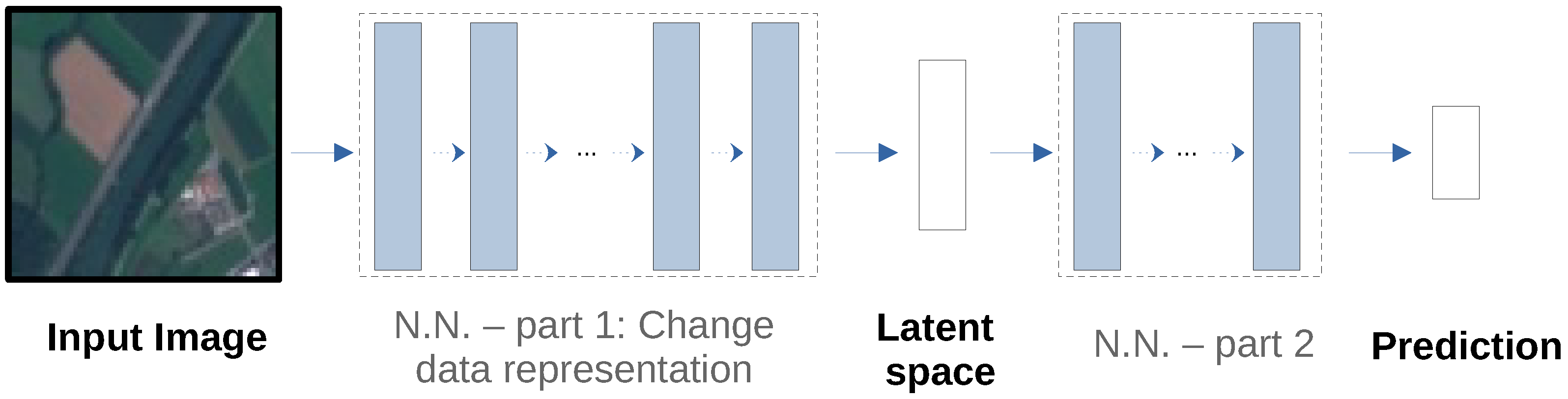
6. A Generic Pipeline to Detect and to Treat Unsuspected Sensitive Variables

We have given, in the previous sections, an overview of the tools to quantify, detect and mitigate undesired algorithmic biases in machine learning, with a particular focus on complex and high-dimensional data such as images. As described in the introduction, we believe that a widely unexplored issue with strong industrial implication is the detection of unsuspected sensitive variables with high-dimensional data. We then present in this section a novel Human-in-the-loop strategy based on Section 4.2 (https://github.com/deel-ai/influenciae, accessed on 30 October 2023) to address this issue. Our pipeline is designed for machine learning models that are trained using a gradient-descent approach (stochastic or not), which is the case for neural network models. It is developed in Algorithm 1, and illustrated in Section 7.
Algorithm 1 Pipeline to detect unsuspected sensitive variables and to mitigate their biases
  • Require: A trained machine learning model f θ .
  • Require: The dataset { x i , y i } i = 1 , , n used to train f θ .
    1:
    Use [93] to quantify the influence γ i > 0 of each observation { x i , y i } on the decisions of f θ . Since f θ is already trained, a high value of γ i indicates that the decision rules of f θ would be particularly impacted by ( x i , y i ) with more training iterations, meaning that the relation between x i and y i is potentially poorly captured by f θ (see Section 4.2).
    2:
    Select the most influential observations, i.e., those with the highest γ i values. The amount of selected observations must be sufficiently small, so that a human can observe all of them. It also has to be sufficiently large to detect whether a significant amount of these observations present similar features.
    3:
    A human then observes the selected observations to define whether a significant amount of them present a common feature.
    4:
    If a common feature is detected in the selected observations, then a sensitive variable A can be defined. Note that this requires to quantify this feature from the input observations x i , which will again be made by using a human intervention.
    5:
    Use the bias metrics of Section 3 with the sensitive variable A to quantify to which extent this sensitive variable is related to an undesired algorithmic bias.
    6:
    If it turns out that f θ is significantly biased with respect to A, the persons in charge of the model optimisation can try understanding the causes of this bias, as explained in Section 2.2, in order to later properly optimise f θ .
    7:
    Alternatively to the previous step, a bias mitigation strategy of Section 5, with A as a sensitive variable, can be directly used.

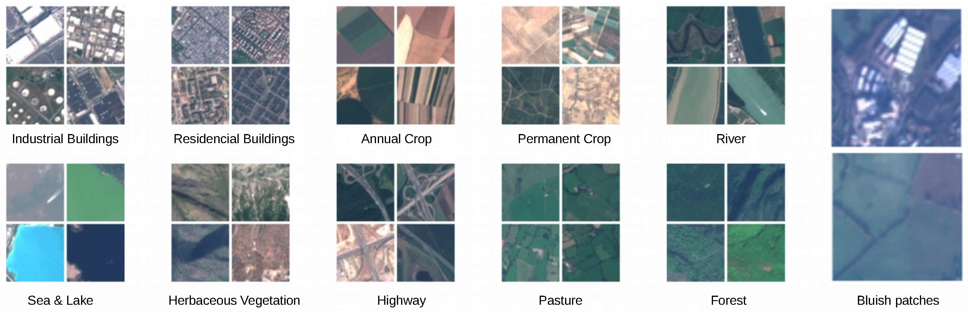
7. A Use-Case for EuroSAT

We now illustrate the notions and concepts of algorithmic bias that can be encountered in industrial applications on the RGB version of the EuroSAT dataset (https://madm.dfki.de/downloads, accessed on 30 October 2023) [5]. It contains 27000 remote sensing images of 64 × 64 pixels with a ground sampling distance of 10 m. The RGB channels were also reconstructed based on the original 13-band Sentinel-2 satellite images. Each image has a label indicating the kind of land it covers, as shown in Figure 2 (left).

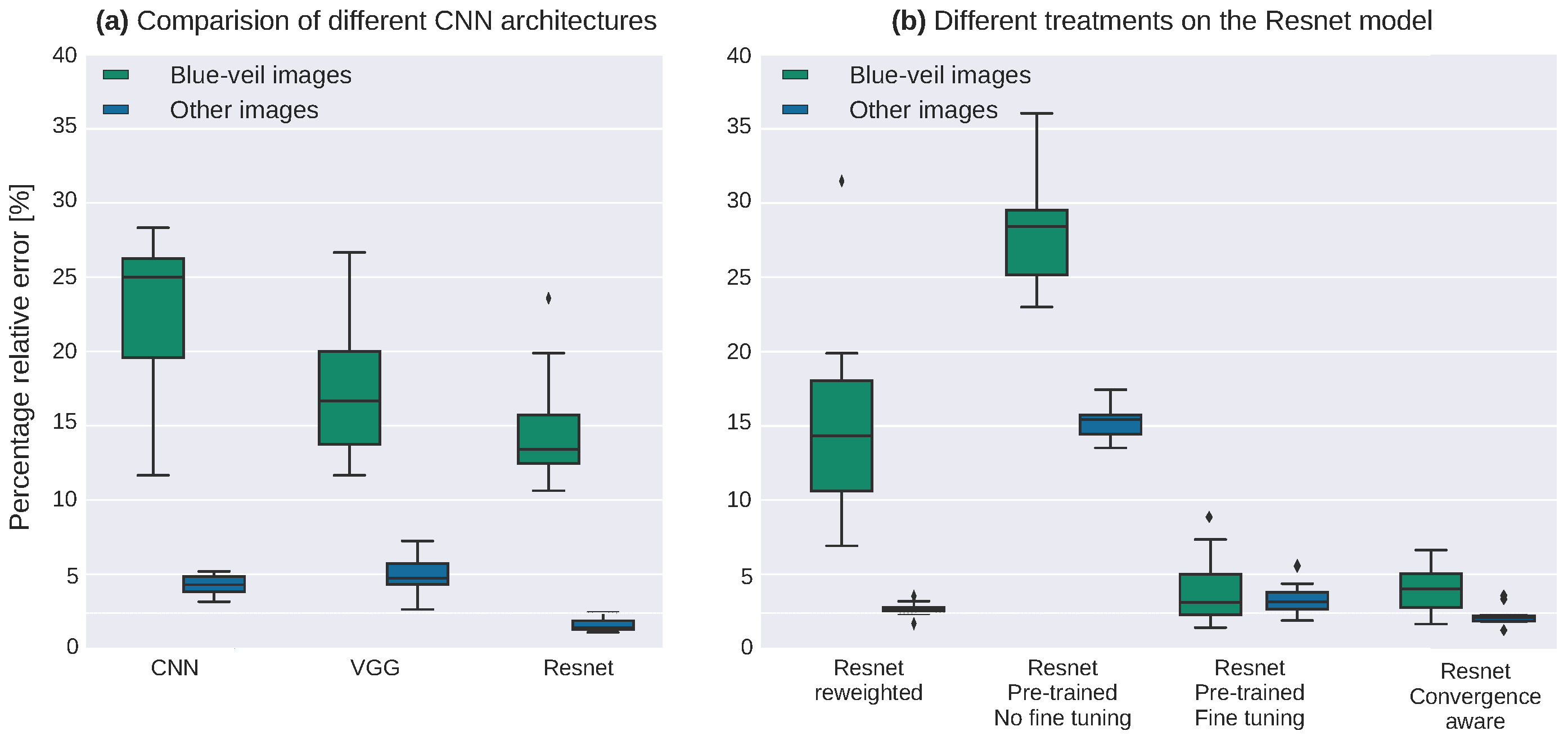
7.1. The Blue Veil Effect in the EuroSAT Dataset

The blue-veil effect is caused by uncommon atmospheric conditions when acquiring Sentinel-2 images on the original 13 spectral bands, and becomes particularly noticeable when they are transformed into the visible spectrum. In essence, the picture acquires a blueish hue, as depicted in Figure 2 (right), that can trick classification models into thinking that it contains a mass of water. About 3% of the dataset is corrupted by what we call the blue-veil effect. Importantly, this blue-veil effect will provide us below a typical example of algorithmic bias with an unknown sensitive variable in high-dimensional data. As we will see, blue-veil images indeed tend to be harder to classify than other images.

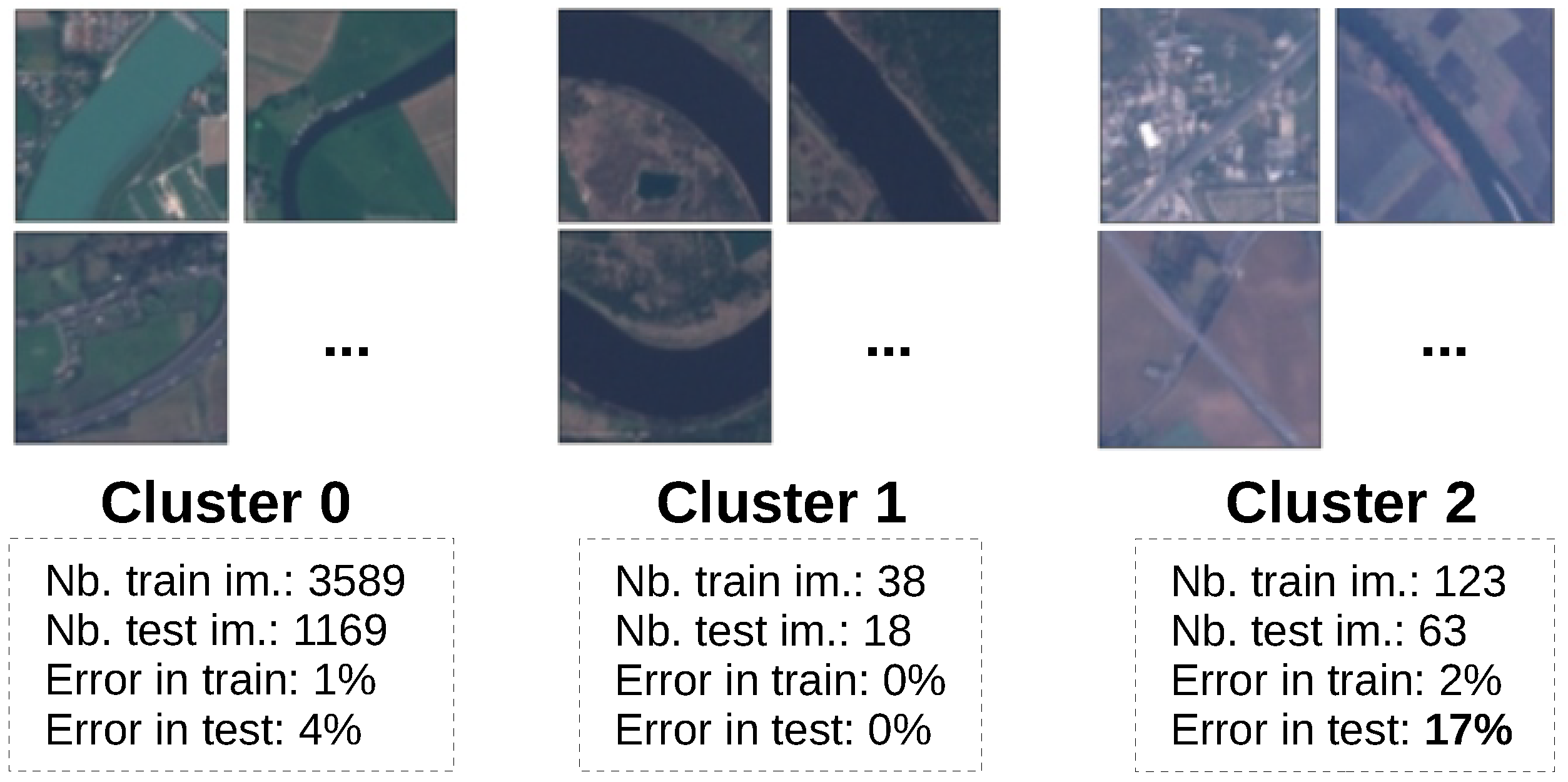
7.2. Detecting Sensitive Variables without Additional Metadata

We explain hereafter how to detect the blue-veil effect as a potential source of bias. The first step is to estimate the importance of each observation of the training dataset for a pre-trained model. This information will then be employed by clustering algorithms on specific image representations in order to automatically find the discriminated group.
We opted for the technique of [93], where first order approximations of NN influence functions were used to determine the importance of each training observation in the trained model. With this objective in mind, a simple and generic 4-layer CNN was trained until convergence. Then, we observed that among the 25 most influential images, 7 of them were blue-veiled images, although such images only represent 3% of the whole dataset. This suggests that training the classifier on blue-veil images is a complex task, or at least that the image features used to classify these images seem to be different from those of the other images.
Since the blue-veil pattern has been semi-automatically identified on several images, we can change the image representation so that a clustering algorithm will straightforwardly find and isolate all the images with this pattern in the training and test sets. For the blue-veiled images, we simply transform the RGB (Red, Green, Blue) colour space into an HSV (Hue, Saturation, Value) space, where the blue-veil images can be characterised by dominant blue colours in the Value channel and reasonably luminous colours in the Hue channel. By using a spectral clustering algorithm on HSV images, we distinguish three image clusters, as shown Figure 3. The first cluster contains normal-looking images, the second one mostly has large and dark rivers, and a last one represents the blue-veiled images we are looking for.

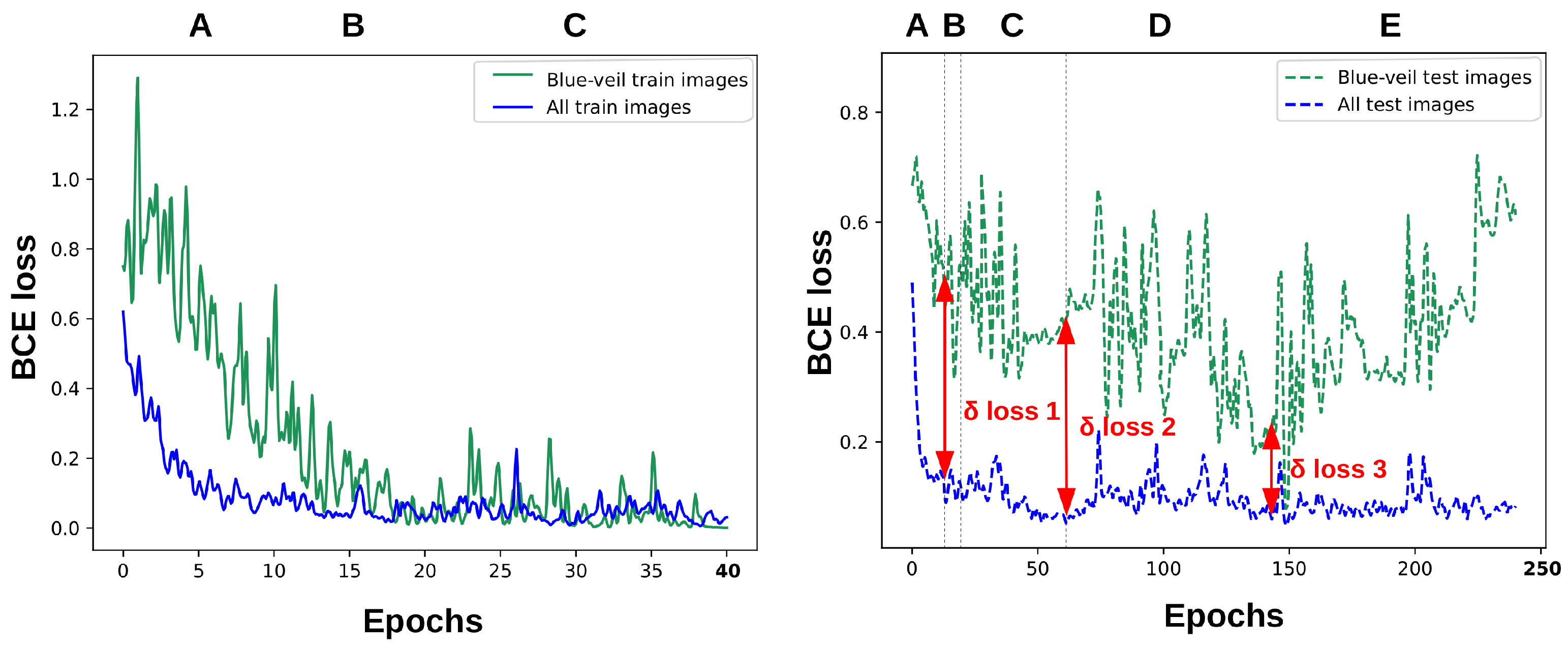
7.3. Measuring the Effect of the Sensitive Variable

Let us check different models’ performances for blue-veiled images and other images. A simple 4-layer CNN, a VGG-16 model, and a ResNet18 model were compared after being trained for 50 epochs. A total of 10 runs per configuration were used to measure the models’ and learning algorithm’s stability. We also focused on the binary classification between Rivers and Highways, which correspond to the two worst performing classes in the 10 class setting. This additionally forced us to train the classifiers with a more limited amount of blue-veiled images, making the problem close to what we can encounter in many industrial applications. The training and test sets indeed contained 3750 and 1250 images, respectively, where only 123 and 63 images were blueish. As shown in Figure 3 and Figure 4a, we can clearly observe that the error rate is considerably higher on blue-veiled images than on other images, thus demonstrating that an undesirable algorithmic bias was learned in the sense of the equality of errors.

7.4. Bias Mitigation

Several strategies to mitigate the undesired bias were also tested. They all used the Resnet18 architecture, as it was the most accurate on blue-veil images (see Figure 4a). Note that we trained the models for 50 epochs by default, just like in the previous subsection. The initial parameters of the neural networks were also randomly drawn, except in two cases that will be mentioned.
We first tested the re-weighting scheme proposed in [106]. The ResNet18 architecture was trained using a weighted loss, where the weights were chosen so that the disparate impact was equal to 1 (reweighted strategy). We also loaded the pre-trained ResNet18 architecture of Torchvision (https://pytorch.org/vision/stable/index.html, accessed on 30 October 2023) and trained its last layer on our EuroSAT data to use the generic transformed image representation of this pre-trained network. It is important to mention that a very large and generic ImageNet database was used for pre-training (Pre-trained, No fine-tuning strategy). We alternatively fine-tuned all layers of this pre-trained network to simultaneously optimise the transformed image representation and the prediction based on this representation, i.e., the parts 1 and 2 of the neural network in Figure 1 (Pre-trained, Fine-tuning strategy). It is important to note that we only trained for 5 epochs instead of 50 when fine-tuning the pre-trained neural networks in order to avoid overfitting. Finally, we randomly drew the initial state of the neural network and trained all layers, but thoroughly distinguished the convergence for all images and for the group of blue-veiled images only. In this case, we stopped training the ResNet18 parameters when an over-fitting phenomenon started being observed in the blue-veiled images (Convergence aware strategy). Results are shown in Figure 4b. A typical detailed convergence of the Convergence aware strategy is also shown in Figure 5.
Finally, we can discuss the results. We can first notice that the re-weighting technique of [106] had little effect on the results. It was indeed designed to correct bias that manifests in the form of disparate impact, so it did not reduce the error rate gap between groups. The debiasing method must then be specifically chosen to target the bias through the metric with which it was measured.
Using the pre-trained network of Torchvision had a disastrous effect when only optimising the last neural network layer, but was particularly efficient when using fine-tuning, i.e., when simultaneously optimising the transformation of the data representation and the final decision rules. Using a relevant initial state, when available, and using fine-tuning then appears as a very good strategy here. This strategy is often denoted by transfer learning in the machine learning literature, and it is widely used when the amount of available data to train a complex neural network is limited. Interestingly, similar results were obtained with a random initial state, when stopping the training procedure at an iteration where the trained neural network had good generalisation properties on the blue-veiled images. Understanding this result requires looking closely at the convergence curves, as illustrated Figure 5 on a typical run.
In Figure 5, we compare the convergence in the whole train and test sets, as well as the blue-veil images only. We can then distinguish five phases in the convergence process. All curves start decreasing in phase A. It can only be remarked that the loss on the blue-veil images slightly increases during the 4 first epochs before decreasing, as in the average trend. We believe that this is due to a minor confounding effect. In phase B, i.e., between epochs 12 and 18, the training algorithm has converged when observed on all training images but not yet on blue-veil images. This is due to the fact that the blue-veil images only represent a small fraction of the training set. Note that if only measuring the convergence on the whole training set, it would be tempting to stop the training process at the beginning of phase B, which would obviously lead to a different treatment of the blue-veiled images and other images (see δ loss 1 in Figure 5). More interestingly for us, the convergence curves are stable on the training set in phase C, but it regularly decreases on the test set. At the end of phase C, the convergence curve is stable on the whole test set, and it is common practice to stop the training process there (early stopping principle). However, it is important to remark that the generalisation properties of the trained neural network are still much poorer for blue-veiled images than other images (see δ loss 2 in Figure 5). This actually explains in Figure 4a the different accuracies observed for the blue-veiled images with respect to the other images. We indeed stopped the convergence after 50 epochs there. Although noisy, the convergence curve obtained on blue-veil test images slowly decreases in phase D until reaching an optimal value at epoch 145 (see δ loss 3 in Figure 5). Finally, the training algorithm starts over-fitting the blue-veiled images in phase E, so the training process should be stopped at its very beginning. It is then essential to point out that obtaining reasonably good generalisation properties on blue-veiled images required about 3 times more epochs than what is made using what is commonly considered to be the good practices, and about 12 times more epochs than what would be made using a naive approach.

8. Conclusions

We have addressed in this paper the issue of algorithmic bias detection and mitigation in machine learning, with a particular focus on complex and high-dimensional data. While, in societal applications, the common sense or new regulations can help the data scientists detecting the sensitive variables related to algorithmic biases, this task can be much more complex in industrial application. The sensitive variables can indeed be unsuspected in this case, as illustrated in our remote sensing use-case, where some training images presented a reconstruction artefact (the blue-veil effect) making the predictions inaccurate.
After stating the various causes of algorithmic bias in machine learning and reviewing the main strategies for measuring, detecting and correcting bias, we then developed in Section 6 a new pipeline to deal with the problem of unknown bias on unsuspected sensitive variables. Interestingly, the application of our pipeline to the use-case of Section 7 additionally pushed us to understand what was the source of the bias on the blue-veil images. In this case, this was due to an insufficient algorithm convergence on this subgroup of images, probably because they were particularly different to other images. We then reframed the problem as an optimizing problem, where we carefully monitored the learning process in order to learn without creating algorithmic bias. This improved learning procedure was, however, only made possible because the unsuspected sensitive variable was identified using our Human-in-the-loop strategy.
To go further than our study, we also believe that an in-depth work is necessary before deploying an AI-based solution, in particular when it will be used for sensitive applications. In that sense, we should see the different regulations arising as an opportunity to gain knowledge on data, deep learning, and optimisation instead of a brake on innovation.
Future work will deal with the extension of our work to Large Language Models, where the possible amount of sensitive variables to detect can be larger than when using conventional industrial training sets. In a sense, this work will require an additional level of abstraction to efficiently use human intelligence in order to robustify the model decisions.

Author Contributions

Conceptualization, L.R., J.-M.L., A.M.P. and L.H.; methodology, L.R., J.-M.L., A.M.P. and L.H.; software, L.R., A.M.P. and L.H.; validation, L.R., A.M.P. and L.H.; formal analysis, L.R., J.-M.L., A.M.P. and L.H.; investigation, L.R., J.-M.L., A.M.P. and L.H.; resources, L.R., A.M.P. and L.H.; data curation, L.R., A.M.P. and L.H.; writing—original draft preparation, L.R., J.-M.L., A.M.P. and L.H.; writing—review and editing, L.R. and J.-M.L.; visualization, A.M.P. and L.R.; supervision, L.R. and J.-M.L.; project administration, J.-M.L.; funding acquisition, J.-M.L. All authors have read and agreed to the published version of the manuscript.

Funding

This work was conducted as part of the DEEL project (www.deel.ai, accessed on 30 October 2023). Funding was provided by ANR-3IA Artificial and Natural Intelligence Toulouse Institute (ANR-19-PI3A-0004).

Data Availability Statement

The EuroSAT dataset is available at the address https://madm.dfki.de/downloads (accessed on 30 October 2023).

Conflicts of Interest

The authors declare no conflict of interest. The funders had no role in the design of the study; in the collection, analyses, or interpretation of data; in the writing of the manuscript; or in the decision to publish the results.

References

  1. Vermeulen, A.F. Industrial Machine Learning, 1st ed.; Apress: Berkeley, CA, USA, 2020. [Google Scholar]
  2. Bertolini, M.; Mezzogori, D.; Neroni, M.; Zammori, F. Machine Learning for industrial applications: A comprehensive literature review. Expert Syst. Appl. 2021, 175, 114820. [Google Scholar] [CrossRef]
  3. Deng, J.; Dong, W.; Socher, R.; Li, L.J.; Li, K.; Li, F.-F. Imagenet: A large-scale hierarchical image database. In Proceedings of the 2009 IEEE Conference on Computer Vision and Pattern Recognition, Miami, FL, USA, 20–25 June 2009; pp. 248–255. [Google Scholar]
  4. LeCun, Y.; Cortes, C.; Burges, C. MNIST Handwritten Digit Database. ATT Labs. Available online: http://yann.lecun.com/exdb/mnist (accessed on 30 October 2023).
  5. Helber, P.; Bischke, B.; Dengel, A.; Borth, D. Eurosat: A novel dataset and deep learning benchmark for land use and land cover classification. IEEE J. Sel. Top. Appl. Earth Obs. Remote Sens. 2019, 12, 2217–2226. [Google Scholar] [CrossRef]
  6. Lin, T.Y.; Maire, M.; Belongie, S.; Hays, J.; Perona, P.; Ramanan, D.; Dollár, P.; Zitnick, C.L. Microsoft coco: Common objects in context. In Proceedings of the European Conference on Computer Vision, Zurich, Switzerland, 6–12 September 2014; pp. 740–755. [Google Scholar]
  7. Cordts, M.; Omran, M.; Ramos, S.; Rehfeld, T.; Enzweiler, M.; Benenson, R.; Franke, U.; Roth, S.; Schiele, B. The Cityscapes Dataset for Semantic Urban Scene Understanding. In Proceedings of the IEEE Conference on Computer Vision and Pattern Recognition (CVPR), Las Vegas, NV, USA, 27–30 June 2016. [Google Scholar]
  8. Koehn, P. Europarl: A Parallel Corpus for Statistical Machine Translation. In Proceedings of the MTSUMMIT, Phuket, Thailand, 6–12 September 2005. [Google Scholar]
  9. Maas, A.L.; Daly, R.E.; Pham, P.T.; Huang, D.; Ng, A.Y.; Potts, C. Learning Word Vectors for Sentiment Analysis. In Proceedings of the 49th Annual Meeting of the Association for Computational Linguistics: Human Language Technologies, Portland, OR, USA, 27–30 June 2011; pp. 142–150. [Google Scholar]
  10. Krizhevsky, A.; Sutskever, I.; Hinton, G.E. Imagenet classification with deep convolutional neural networks. Adv. Neural Inf. Process. Syst. 2012, 25, 12. [Google Scholar] [CrossRef]
  11. Simonyan, K.; Zisserman, A. Very Deep Convolutional Networks for Large-Scale Image Recognition. In Proceedings of the 3rd International Conference on Learning Representations, ICLR, San Diego, CA, USA, 7–9 May 2015. [Google Scholar]
  12. He, K.; Zhang, X.; Ren, S.; Sun, J. Deep residual learning for image recognition. In Proceedings of the IEEE Conference on Computer Vision and Pattern Recognition, Seattle, WA, USA, 14–19 June 2016; pp. 770–778. [Google Scholar]
  13. Ioffe, S.; Szegedy, C. Batch normalization: Accelerating deep network training by reducing internal covariate shift. In Proceedings of the International Conference on Machine Learning, PMLR, Lille, France, 7–9 July 2015; pp. 448–456. [Google Scholar]
  14. LeCun, Y.; Bottou, L.; Bengio, Y.; Haffner, P. Gradient-Based Learning Applied to Document Recognition. Proc. IEEE 1998, 86, 2278–2324. [Google Scholar] [CrossRef]
  15. Vaswani, A.; Shazeer, N.; Parmar, N.; Uszkoreit, J.; Jones, L.; Gomez, A.N.; Kaiser, L.U.; Polosukhin, I. Attention is All you Need. In Proceedings of the Advances in Neural Information Processing Systems, Long Beach, CA, USA, 27–30 June 2017; Volume 30. [Google Scholar]
  16. LeCun, Y.A.; Bottou, L.; Orr, G.B.; Müller, K.R. Efficient BackProp. In Neural Networks: Tricks of the Trade: Second Edition; Montavon, G., Orr, G.B., Muller, K.R., Eds.; Springer: Berlin/Heidelberg, Germany, 2012; pp. 9–48. [Google Scholar]
  17. Arora, R.; Basu, A.; Mianjy, P.; Mukherjee, A. Understanding Deep Neural Networks with Rectified Linear Units. In Proceedings of the International Conference on Learning Representations, Vancouver, BC, Canada, 30 April–3 May 2018. [Google Scholar]
  18. Kingma, D.P.; Welling, M. Auto-Encoding Variational Bayes. In Proceedings of the 2nd International Conference on Learning Representations, ICLR 2014, Banff, AB, Canada, 14–16 April 2014. [Google Scholar]
  19. Ronneberger, O.; Fischer, P.; Brox, T. U-Net: Convolutional Networks for Biomedical Image Segmentation. In Proceedings of the Medical Image Computing and Computer-Assisted Intervention—MICCAI 2015, Munich, Germany, 5–9 October 2015; Navab, N., Hornegger, J., Wells, W.M., Frangi, A.F., Eds.; Springer: Berlin/Heidelberg, Germany, 2015; pp. 234–241. [Google Scholar]
  20. Selvaraju, R.R.; Cogswell, M.; Das, A.; Vedantam, R.; Parikh, D.; Batra, D. Grad-cam: Visual explanations from deep networks via gradient-based localization. In Proceedings of the IEEE International Conference on Computer Vision, Venice, Italy, 22–29 October 2017; pp. 618–626. [Google Scholar]
  21. Fel, T.; Cadène, R.; Chalvidal, M.; Cord, M.; Vigouroux, D.; Serre, T. Look at the Variance! Efficient Black-box Explanations with Sobol-based Sensitivity Analysis. Adv. Neural Inf. Process. Syst. 2021, 34, 21. [Google Scholar]
  22. Ribeiro, M.T.; Singh, S.; Guestrin, C. Why should i trust you? Explaining the predictions of any classifier. In Proceedings of the 22nd ACM SIGKDD International Conference on Knowledge Discovery and Data Mining, San Francisco, CA, USA, 13–17 July 2016; pp. 1135–1144. [Google Scholar]
  23. Olah, C.; Mordvintsev, A.; Schubert, L. Feature Visualization. Distill 2017, 2017, 7. [Google Scholar] [CrossRef]
  24. Jourdan, F.; Picard, A.; Fel, T.; Risser, L.; Loubes, J.M.; Asher, N. COCKATIEL: COntinuous Concept ranKed ATtribution with Interpretable ELements for explaining neural net classifiers on NLP tasks. arXiv 2023, arXiv:2305.06754. [Google Scholar]
  25. Lee, K.; Lee, K.; Lee, H.; Shin, J. A simple unified framework for detecting out-of-distribution samples and adversarial attacks. Adv. Neural Inf. Process. Syst. 2018, 31, 18. [Google Scholar]
  26. Nalisnick, E.; Matsukawa, A.; Teh, Y.W.; Gorur, D.; Lakshminarayanan, B. Do deep generative models know what they don’t know? arXiv 2018, arXiv:1810.09136. [Google Scholar]
  27. Castelnovo, A.; Crupi, R.; Greco, G.; Regoli, D.; Penco, I.G.; Cosentini, A.C. A clarification of the nuances in the fairness metrics landscape. Nat. Sci. Rep. 2022, 12, 22. [Google Scholar] [CrossRef]
  28. Pessach, D.; Shmueli, E. A Review on Fairness in Machine Learning. ACM Comput. Surv. 2022, 55, 23. [Google Scholar] [CrossRef]
  29. Kusner, M.; Loftus, J.; Russell, C.; Silva, R. Counterfactual Fairness. In Proceedings of the 31st International Conference on Neural Information Processing Systems, Long Beach, CA, USA, 4–9 December 2017; pp. 4069–4079. [Google Scholar]
  30. De Lara, L.; González-Sanz, A.; Asher, N.; Loubes, J.M. Transport-based counterfactual models. arXiv 2021, arXiv:2108.13025. [Google Scholar]
  31. Garvie, C.; Frankle, J. Facial-recognition software might have a racial bias problem. The Atlantic 2016, 7, 16. [Google Scholar]
  32. Castelvecchi, D. Is facial recognition too biased to be let loose? Nature 2020, 587, 347–350. [Google Scholar] [CrossRef] [PubMed]
  33. Conti, J.R.; Noiry, N.; Clemencon, S.; Despiegel, V.; Gentric, S. Mitigating Gender Bias in Face Recognition using the von Mises-Fisher Mixture Model. In Proceedings of the International Conference on Machine Learning, PMLR, Baltimore, MA, USA, 17–23 July 2022; pp. 4344–4369. [Google Scholar]
  34. Liu, Z.; Luo, P.; Wang, X.; Tang, X. Deep Learning Face Attributes in the Wild. In Proceedings of the International Conference on Computer Vision (ICCV), Paris, France, 2–4 December 2015. [Google Scholar]
  35. Kuznetsova, A.; Rom, H.; Alldrin, N.; Uijlings, J.; Krasin, I.; Pont-Tuset, J.; Kamali, S.; Popov, S.; Malloci, M.; Kolesnikov, A.; et al. The Open Images Dataset V4. Int. J. Comput. Vis. 2020, 128, 1956–1981. [Google Scholar] [CrossRef]
  36. Fabris, A.; Messina, S.; Silvello, G.; Susto, G.A. Algorithmic Fairness Datasets: The Story so Far. arXiv 2022, arXiv:2202.01711. [Google Scholar] [CrossRef]
  37. Shankar, S.; Halpern, Y.; Breck, E.; Atwood, J.; Wilson, J.; Sculley, D. No classification without representation: Assessing geodiversity issues in open data sets for the developing world. arXiv 2017, arXiv:1711.08536. [Google Scholar]
  38. Riccio, P.; Oliver, N. Racial Bias in the Beautyverse. arXiv 2022, arXiv:2209.13939. [Google Scholar]
  39. Buolamwini, J.; Gebru, T. Gender shades: Intersectional accuracy disparities in commercial gender classification. In Proceedings of the Conference on Fairness, Accountability and Transparency, PMLR, Baltimore, MA, USA, 17–23 June 2018; pp. 77–91. [Google Scholar]
  40. Merler, M.; Ratha, N.; Feris, R.S.; Smith, J.R. Diversity in faces. arXiv 2019, arXiv:1901.10436. [Google Scholar]
  41. Karkkainen, K.; Joo, J. Fairface: Face attribute dataset for balanced race, gender, and age for bias measurement and mitigation. In Proceedings of the IEEE/CVF Winter Conference on Applications of Computer Vision, Waikoloa, HI, USA, 3–7 July 2021; pp. 1548–1558. [Google Scholar]
  42. Johnson, A.E.; Pollard, T.J.; Greenbaum, N.R.; Lungren, M.P.; Deng, C.Y.; Peng, Y.; Lu, Z.; Mark, R.G.; Berkowitz, S.J.; Horng, S. MIMIC-CXR-JPG, a large publicly available database of labeled chest radiographs. arXiv 2019, arXiv:1901.07042. [Google Scholar]
  43. Irvin, J.; Rajpurkar, P.; Ko, M.; Yu, Y.; Ciurea-Ilcus, S.; Chute, C.; Marklund, H.; Haghgoo, B.; Ball, R.; Shpanskaya, K.; et al. Chexpert: A large chest radiograph dataset with uncertainty labels and expert comparison. Proc. AAAI Conf. Artif. Intell. 2019, 33, 590–597. [Google Scholar] [CrossRef]
  44. Tschandl, P.; Rosendahl, C.; Kittler, H. The HAM10000 dataset, a large collection of multi-source dermatoscopic images of common pigmented skin lesions. Sci. Data 2018, 5, 1–9. [Google Scholar] [CrossRef] [PubMed]
  45. Guo, L.N.; Lee, M.S.; Kassamali, B.; Mita, C.; Nambudiri, V.E. Bias in, bias out: Underreporting and underrepresentation of diverse skin types in machine learning research for skin cancer detection—A scoping review. J. Am. Acad. Dermatol. 2021, 87, 157–159. [Google Scholar] [CrossRef] [PubMed]
  46. Bevan, P.J.; Atapour-Abarghouei, A. Skin Deep Unlearning: Artefact and Instrument Debiasing in the Context of Melanoma Classification. arXiv 2021, arXiv:2109.09818. [Google Scholar]
  47. Huang, J.; Galal, G.; Etemadi, M.; Vaidyanathan, M. Evaluation and Mitigation of Racial Bias in Clinical Machine Learning Models: Scoping Review. JMIR Med. Inform. 2022, 10, e36388. [Google Scholar] [CrossRef]
  48. Ross, C.; Katz, B.; Barbu, A. Measuring social biases in grounded vision and language embeddings. In Proceedings of the NAACL, Mexico City, Mexico, 6–11 June 2021. [Google Scholar]
  49. Singh, K.K.; Mahajan, D.; Grauman, K.; Lee, Y.J.; Feiszli, M.; Ghadiyaram, D. Don’t judge an object by its context: Learning to overcome contextual bias. In Proceedings of the IEEE/CVF Conference on Computer Vision and Pattern Recognition, Seattle, WA, USA, 13–19 June 2020; pp. 11070–11078. [Google Scholar]
  50. Saffarian, S.; Elson, E. Statistical analysis of fluorescence correlation spectroscopy: The standard deviation and bias. Biophys. J. 2003, 84, 2030–2042. [Google Scholar] [CrossRef] [PubMed]
  51. Tschandl, P. Risk of Bias and Error From Data Sets Used for Dermatologic Artificial Intelligence. JAMA Dermatol. 2021, 157, 1271–1273. [Google Scholar] [CrossRef]
  52. Pawlowski, N.; Coelho de Castro, D.; Glocker, B. Deep structural causal models for tractable counterfactual inference. Adv. Neural Inf. Process. Syst. 2020, 33, 857–869. [Google Scholar]
  53. Brown, T.B.; Mann, B.; Ryder, N.; Subbiah, M.; Kaplan, J.; Dhariwal, P.; Neelakantan, A.; Shyam, P.; Sastry, G.; Askell, A.; et al. Language Models are Few-Shot Learners. arXiv 2020, arXiv:cs.CL/2005.14165. [Google Scholar]
  54. Lucy, L.; Bamman, D. Gender and representation bias in GPT-3 generated stories. In Proceedings of the Third Workshop on Narrative Understanding, San Francisco, CA, USA, 15 June 2021; pp. 48–55. [Google Scholar]
  55. Locatello, F.; Abbati, G.; Rainforth, T.; Bauer, S.; Scholkopf, B.; Bachem, O. On the Fairness of Disentangled Representations. In Proceedings of the 33rd International Conference on Neural Information Processing Systems, Vancouver, BC, Canada, 6–12 December 2019. [Google Scholar]
  56. Fjeld, J.; Achten, N.; Hilligoss, H.; Nagy, A.; Srikumar, M. Principled Artificial Intelligence: Mapping Consensus in Ethical and Rights-based Approaches to Principles for AI. Berkman Klein Cent. Internet Soc. 2022, 2022, 1. [Google Scholar] [CrossRef]
  57. Banerjee, I.; Bhimireddy, A.R.; Burns, J.L.; Celi, L.A.; Chen, L.; Correa, R.; Dullerud, N.; Ghassemi, M.; Huang, S.; Kuo, P.; et al. Reading Race: AI Recognises Patient’s Racial Identity In Medical Images. arXiv 2021, arXiv:abs/2107.10356. [Google Scholar]
  58. Durán, J.M.; Jongsma, K.R. Who is afraid of black box algorithms? On the epistemological and ethical basis of trust in medical AI. J. Med. Ethics 2021, 47, 329–335. [Google Scholar] [CrossRef] [PubMed]
  59. Muehlematter, U.J.; Daniore, P.; Vokinger, K.N. Approval of artificial intelligence and machine learning-based medical devices in the USA and Europe (2015–20): A comparative analysis. Lancet Digit. Health 2021, 3, e195–e203. [Google Scholar] [CrossRef] [PubMed]
  60. Holzinger, A.; Biemann, C.; Pattichis, C.S.; Kell, D.B. What do we need to build explainable AI systems for the medical domain? arXiv 2017, arXiv:abs/1712.09923. [Google Scholar]
  61. Raji, I.D.; Gebru, T.; Mitchell, M.; Buolamwini, J.; Lee, J.; Denton, E. Saving Face: Investigating the Ethical Concerns of Facial Recognition Auditing. In Proceedings of the AAAI/ACM Conference on AI, Ethics, and Society, New York, NY, USA, 6–12 July 2020; pp. 145–151. [Google Scholar] [CrossRef]
  62. Xu, T.; White, J.; Kalkan, S.; Gunes, H. Investigating Bias and Fairness in Facial Expression Recognition. arXiv 2020, arXiv:abs/2007.10075. [Google Scholar]
  63. Atzori, A.; Fenu, G.; Marras, M. Explaining Bias in Deep Face Recognition via Image Characteristics. IJCB 2022, 2022, 110099. [Google Scholar] [CrossRef]
  64. Hardt, M.; Price, E.; Srebro, N. Equality of opportunity in supervised learning. In Proceedings of the Advances in Neural Information Processing Systems, New York, NY, USA, 6–12 July 2016; pp. 3315–3323. [Google Scholar]
  65. Oneto, L.; Chiappa, S. Fairness in Machine Learning. In Recent Trends in Learning From Data; Springer: Berlin/Heidelberg, Germany, 2020; pp. 155–196. [Google Scholar]
  66. Del Barrio, E.; Gordaliza, P.; Loubes, J.M. Review of Mathematical frameworks for Fairness in Machine Learning. arXiv 2020, arXiv:2005.13755. [Google Scholar]
  67. Chouldechova, A.; Roth, A. A snapshot of the frontiers of fairness in machine learning. Commun. ACM 2020, 63, 82–89. [Google Scholar] [CrossRef]
  68. Feldman, M.; Friedler, S.; Moeller, J.; Scheidegger, C.; Venkatasubramanian, S. Certifying and removing disparate impact. In Proceedings of the 21th ACM SIGKDD International Conference on Knowledge Discovery and Data Mining, Sydney, NSW, Australia, 10–13 August 2015. [Google Scholar]
  69. Zafar, M.B.; Valera, I.; Gomez Rodriguez, M.; Gummadi, K.P. Fairness beyond disparate treatment & disparate impact: Learning classification without disparate mistreatment. In Proceedings of the 26th International Conference on World Wide Web, International World Wide Web Conferences Steering Committee, Perth, Australia, 3–7 April 2017; pp. 1171–1180. [Google Scholar]
  70. Gordaliza, P.; Del Barrio, E.; Gamboa, F.; Loubes, J.M. Obtaining Fairness using Optimal Transport Theory. In Proceedings of the International Conference on Machine Learning (ICML), Virtual Event, 13–18 July 2019; pp. 2357–2365. [Google Scholar]
  71. Chouldechova, A. Fair Prediction with Disparate Impact: A Study of Bias in Recidivism Prediction Instruments. Big Data 2017, 5, 17. [Google Scholar] [CrossRef]
  72. Pleiss, G.; Raghavan, M.; Wu, F.; Kleinberg, J.; Weinberger, K.Q. On Fairness and Calibration. In Proceedings of the Advances in Neural Information Processing Systems, Long Beach, CA, USA, 4–9 December 2017; Volume 30. [Google Scholar]
  73. Barocas, S.; Hardt, M.; Narayanan, A. Fairness in machine learning. Nips Tutor. 2017, 1, 2. [Google Scholar]
  74. Yang, D.; Lafferty, J.; Pollard, D. Fair quantile regression. arXiv 2019, arXiv:1907.08646. [Google Scholar]
  75. Bénesse, C.; Gamboa, F.; Loubes, J.M.; Boissin, T. Fairness seen as global sensitivity analysis. Mach. Learn. 2022, 2022, 1–28. [Google Scholar] [CrossRef]
  76. Ghosh, B.; Basu, D.; Meel, K.S. How Biased is Your Feature? Computing Fairness Influence Functions with Global Sensitivity Analysis. arXiv 2022, arXiv:2206.00667. [Google Scholar]
  77. Kamishima, T.; Akaho, S.; Sakuma, J. Fairness-aware learning through regularization approach. In Proceedings of the 2011 IEEE 11th International Conference on Data Mining Workshops, Vancouver, BC, Canada, 11 December 2011; pp. 643–650. [Google Scholar]
  78. Risser, L.; Sanz, A.G.; Vincenot, Q.; Loubes, J.M. Tackling Algorithmic Bias in Neural-Network Classifiers Using Wasserstein-2 Regularization. J. Math. Imaging Vis. 2022, 64, 672–689. [Google Scholar] [CrossRef]
  79. Oneto, L.; Donini, M.; Luise, G.; Ciliberto, C.; Maurer, A.; Pontil, M. Exploiting MMD and Sinkhorn Divergences for Fair and Transferable Representation Learning. In Proceedings of the 34th International Conference on Neural Information Processing Systems, Red Hook, NY, USA, 14 December 2020. [Google Scholar]
  80. Serna, I.; Pena, A.; Morales, A.; Fierrez, J. InsideBias: Measuring bias in deep networks and application to face gender biometrics. In Proceedings of the 2020 25th International Conference on Pattern Recognition (ICPR), Milano, Italy, 10–15 January 2021; pp. 3720–3727. [Google Scholar]
  81. Serna, I.; Morales, A.; Fierrez, J.; Ortega-Garcia, J. IFBiD: Inference-free bias detection. arXiv 2021, arXiv:2109.04374. [Google Scholar]
  82. Creager, E.; Jacobsen, J.; Zemel, R.S. Exchanging Lessons Between Algorithmic Fairness and Domain Generalization. arXiv 2020, arXiv:abs/2010.07249. [Google Scholar]
  83. Sohoni, N.S.; Dunnmon, J.A.; Angus, G.; Gu, A.; Ré, C. No Subclass Left Behind: Fine-Grained Robustness in Coarse-Grained Classification Problems. arXiv 2020, arXiv:abs/2011.12945. [Google Scholar]
  84. Matsuura, T.; Harada, T. Domain Generalization Using a Mixture of Multiple Latent Domains. arXiv 2019, arXiv:abs/1911.07661. [Google Scholar] [CrossRef]
  85. Ahmed, F.; Bengio, Y.; van Seijen, H.; Courville, A.C. Systematic generalisation with group invariant predictions. In Proceedings of the ICLR, Virtual Event, 3–7 May 2021. [Google Scholar]
  86. Denton, E.; Hutchinson, B.; Mitchell, M.; Gebru, T. Detecting bias with generative counterfactual face attribute augmentation. arXiv 2019, arXiv:1906.06439. [Google Scholar]
  87. Li, Z.; Xu, C. Discover the Unknown Biased Attribute of an Image Classifier. In Proceedings of the IEEE/CVF International Conference on Computer Vision, Montreal, QC, Canada, 10–17 October 2021; pp. 14970–14979. [Google Scholar]
  88. Paul, W.; Burlina, P. Generalizing Fairness: Discovery and Mitigation of Unknown Sensitive Attributes. arXiv 2021, arXiv:abs/2107.13625. [Google Scholar]
  89. Tong, S.; Kagal, L. Investigating bias in image classification using model explanations. arXiv 2020, arXiv:2012.05463. [Google Scholar]
  90. Schaaf, N.; Mitri, O.D.; Kim, H.B.; Windberger, A.; Huber, M.F. Towards measuring bias in image classification. In Proceedings of the International Conference on Artificial Neural Networks, Bratislava, Slovakia, 14–17 September 2021; Springer: Berlin/Heidelberg, Germany, 2021; pp. 433–445. [Google Scholar]
  91. Sirotkin, K.; Carballeira, P.; Escudero-Viñolo, M. A study on the distribution of social biases in self-supervised learning visual models. In Proceedings of the IEEE/CVF Conference on Computer Vision and Pattern Recognition, New Orleans, LA, USA, 18–24 June 2022; pp. 10442–10451. [Google Scholar]
  92. Bao, Y.; Barzilay, R. Learning to Split for Automatic Bias Detection. arXiv 2022, arXiv:abs/2204.13749. [Google Scholar]
  93. Picard, A.M.; Vigouroux, D.; Zamolodtchikov, P.; Vincenot, Q.; Loubes, J.M.; Pauwels, E. Leveraging Influence Functions for Dataset Exploration and Cleaning. In Proceedings of the 11th European Congress Embedded Real Time Systems (ERTS 2022), Toulouse, France, 13 April 2022; pp. 1–8. [Google Scholar]
  94. Mohler, G.; Raje, R.; Carter, J.; Valasik, M.; Brantingham, J. A penalized likelihood method for balancing accuracy and fairness in predictive policing. In Proceedings of the 2018 IEEE International Conference on Systems, Man, and Cybernetics (SMC), Tokyo, Japan, 7–10 October 2018; pp. 2454–2459. [Google Scholar]
  95. Castets-Renard, C.; Besse, P.; Loubes, J.M.; Perrussel, L. Technical and Legal Risk Management of Predictive Policing Activities; French Ministère de l’intérieur: Paris, France, 2019. [Google Scholar]
  96. Balagopalan, A.; Zhang, H.; Hamidieh, K.; Hartvigsen, T.; Rudzicz, F.; Ghassemi, M. The Road to Explainability is Paved with Bias: Measuring the Fairness of Explanations. arXiv 2022, arXiv:2205.03295. [Google Scholar]
  97. Dai, J.; Upadhyay, S.; Aivodji, U.; Bach, S.H.; Lakkaraju, H. Fairness via Explanation Quality: Evaluating Disparities in the Quality of Post hoc Explanations. arXiv 2022, arXiv:2205.07277. [Google Scholar]
  98. Seo, S.; Lee, J.Y.; Han, B. Unsupervised Learning of Debiased Representations with Pseudo-Attributes. In Proceedings of the IEEE/CVF Conference on Computer Vision and Pattern Recognition, Las Vegas, NV, USA, 14–17 July 2022; pp. 16742–16751. [Google Scholar]
  99. Duchi, J.C.; Namkoong, H. Learning models with uniform performance via distributionally robust optimization. Ann. Stat. 2021, 49, 1378–1406. [Google Scholar] [CrossRef]
  100. Zhang, B.H.; Lemoine, B.; Mitchell, M. Mitigating unwanted biases with adversarial learning. In Proceedings of the 2018 AAAI/ACM Conference on AI, Ethics, and Society, New Orleans, LA, USA, 2–3 February 2018; pp. 335–340. [Google Scholar]
  101. Kim, B.; Kim, H.; Kim, K.; Kim, S.; Kim, J. Learning not to learn: Training deep neural networks with biased data. In Proceedings of the IEEE/CVF Conference on Computer Vision and Pattern Recognition, New Orleans, LA, USA, 18–22 June 2019; pp. 9012–9020. [Google Scholar]
  102. Grari, V.; Ruf, B.; Lamprier, S.; Detyniecki, M. Fairness-Aware Neural Rényi Minimization for Continuous Features. IJCAI 2020, 19, 15. [Google Scholar]
  103. Perez-Suay, A.; Gordaliza, P.; Loubes, J.M.; Sejdinovic, D.; Camps-Valls, G. Fair Kernel Regression through Cross-Covariance Operators. Trans. Mach. Learn. Res. 2023, 13, 23. [Google Scholar]
  104. Creager, E.; Madras, D.; Jacobsen, J.H.; Weis, M.; Swersky, K.; Pitassi, T.; Zemel, R. Flexibly fair representation learning by disentanglement. In Proceedings of the International Conference on Machine Learning, PMLR, Long Beach, CA, USA, 9–15 June 2019; pp. 1436–1445. [Google Scholar]
  105. Sarhan, M.H.; Navab, N.; Eslami, A.; Albarqouni, S. Fairness by learning orthogonal disentangled representations. In Proceedings of the European Conference on Computer Vision, Glasgow, UK, 23–28 August 2020; pp. 746–761. [Google Scholar]
  106. Kamiran, F.; Calders, T. Data preprocessing techniques for classification without discrimination. Knowl. Inf. Syst. 2012, 33, 1–33. [Google Scholar] [CrossRef]
  107. Sagawa, S.; Raghunathan, A.; Koh, P.W.; Liang, P. An investigation of why overparameterization exacerbates spurious correlations. In Proceedings of the International Conference on Machine Learning, PMLR, Virtual Event, 13–18 June 2020; pp. 8346–8356. [Google Scholar]
  108. Buda, M.; Maki, A.; Mazurowski, M.A. A systematic study of the class imbalance problem in convolutional neural networks. Neural Netw. 2018, 106, 249–259. [Google Scholar] [CrossRef]
  109. Zhang, H.; Cisse, M.; Dauphin, Y.N.; Lopez-Paz, D. mixup: Beyond empirical risk minimization. arXiv 2017, arXiv:1710.09412. [Google Scholar]
  110. Du, M.; Mukherjee, S.; Wang, G.; Tang, R.; Awadallah, A.; Hu, X. Fairness via representation neutralization. Adv. Neural Inf. Process. Syst. 2021, 34, 12091–12103. [Google Scholar]
  111. Goel, K.; Gu, A.; Li, Y.; Ré, C. Model patching: Closing the subgroup performance gap with data augmentation. In Proceedings of the ICLR, Virtual Event, 3–7 May 2021. [Google Scholar]
  112. Ramaswamy, V.V.; Kim, S.S.; Russakovsky, O. Fair attribute classification through latent space de-biasing. In Proceedings of the IEEE/CVF Conference on Computer Vision and Pattern Recognition, New Orleans, LA, USA, 18–24 June 2021; pp. 9301–9310. [Google Scholar]
  113. Lee, J.; Kim, E.; Lee, J.; Lee, J.; Choo, J. Learning debiased representation via disentangled feature augmentation. Adv. Neural Inf. Process. Syst. 2021, 34, 25123–25133. [Google Scholar]
  114. Jeon, M.; Kim, D.; Lee, W.; Kang, M.; Lee, J. A Conservative Approach for Unbiased Learning on Unknown Biases. In Proceedings of the IEEE/CVF Conference on Computer Vision and Pattern Recognition, New Orleans, LA, USA, 18–24 June 2022; pp. 16752–16760. [Google Scholar]
  115. Grari, V.; Lamprier, S.; Detyniecki, M. Fairness without the sensitive attribute via Causal Variational Autoencoder. IJCAI 2022, 2022, 3. [Google Scholar]
  116. Zhai, R.; Dan, C.; Suggala, A.; Kolter, J.Z.; Ravikumar, P. Boosted CVaR Classification. Adv. Neural Inf. Process. Syst. 2021, 34, 21860–21871. [Google Scholar]
  117. Sinha, A.; Namkoong, H.; Volpi, R.; Duchi, J. Certifying some distributional robustness with principled adversarial training. arXiv 2017, arXiv:1710.10571. [Google Scholar]
  118. Michel, P.; Hashimoto, T.; Neubig, G. Modeling the second player in distributionally robust optimization. arXiv 2021, arXiv:2103.10282. [Google Scholar]
Figure 1. General architecture of a neural network designed for classification or regression tasks on images. It first projects the input image information non-linearly into a latent space, and then uses this transformed information for its prediction.
Algorithms 16 00510 g001
Figure 2. (Left) Images out of the 10 classes of the EuroSAT dataset. Illustration taken from [5]. (Right) Images of the EuroSAT dataset for which the reconstruction in the RGB colour space produced the blue-veil effect.
Algorithms 16 00510 g002
Figure 3. Detection of potentially discriminated groups and confirmation of blue-veiled images using a clustering and group-wise performance evaluation methodology. The generalisation properties of a ResNet18 classifier in cluster 2, i.e., for blue-veil images, are particularly lower than in the two other clusters.
Algorithms 16 00510 g003
Figure 4. Box-plots of the average errors obtained on the test set with the EuroSat dataset using different models and different training strategies. For each strategy, the two boxplots distinguish the average errors on blue-veiled images (green boxplots) and other images (blue boxplots): (a) Baseline results obtained on different neural network architectures; (b) Effect of different treatments on the average accuracy of the Resnet architecture.
Algorithms 16 00510 g004
Figure 5. Detailed convergence of the BCE-loss on all data and on blue-veil images only. Results obtained on the training set (left) and on the test set (right) are represented. Note that the convergence curves obtained on the training set are only represented for the first 40 epochs, and those obtained on the test set are represented on 250 epochs. Five phases A to E are distinguished to discuss the convergence behaviour.
Algorithms 16 00510 g005
Disclaimer/Publisher’s Note: The statements, opinions and data contained in all publications are solely those of the individual author(s) and contributor(s) and not of MDPI and/or the editor(s). MDPI and/or the editor(s) disclaim responsibility for any injury to people or property resulting from any ideas, methods, instructions or products referred to in the content.

