
Remote Sensing of Snow Parameters: A Sensitivity Study of Retrieval Performance Based on Hyperspectral versus Multispectral Data

Abstract
:1. Introduction
2. Models and Data
2.1. Motivation
2.2. Radiative Transfer Model: AccuRT
2.2.1. Atmospheric Gases
2.2.2. Atmospheric Aerosols
2.2.3. Snow Properties
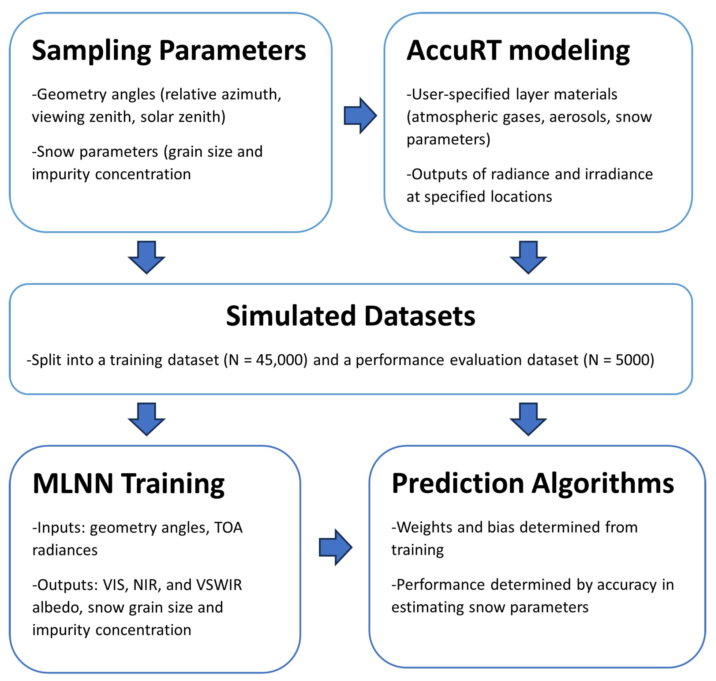
2.3. Synthetic Snow Dataset
2.3.1. Random Data
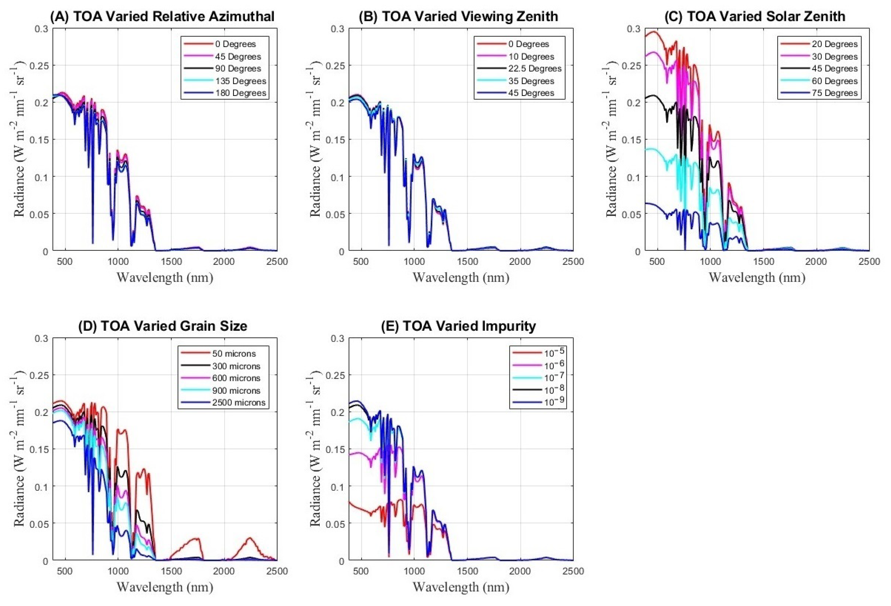
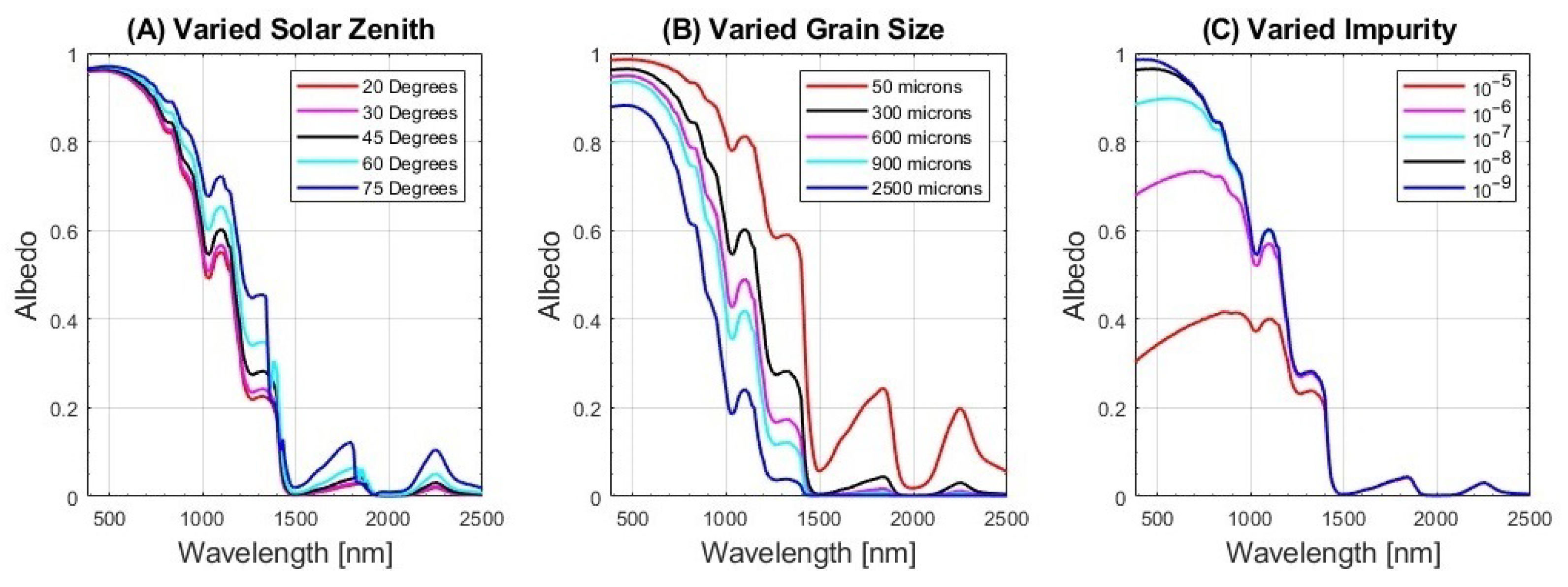
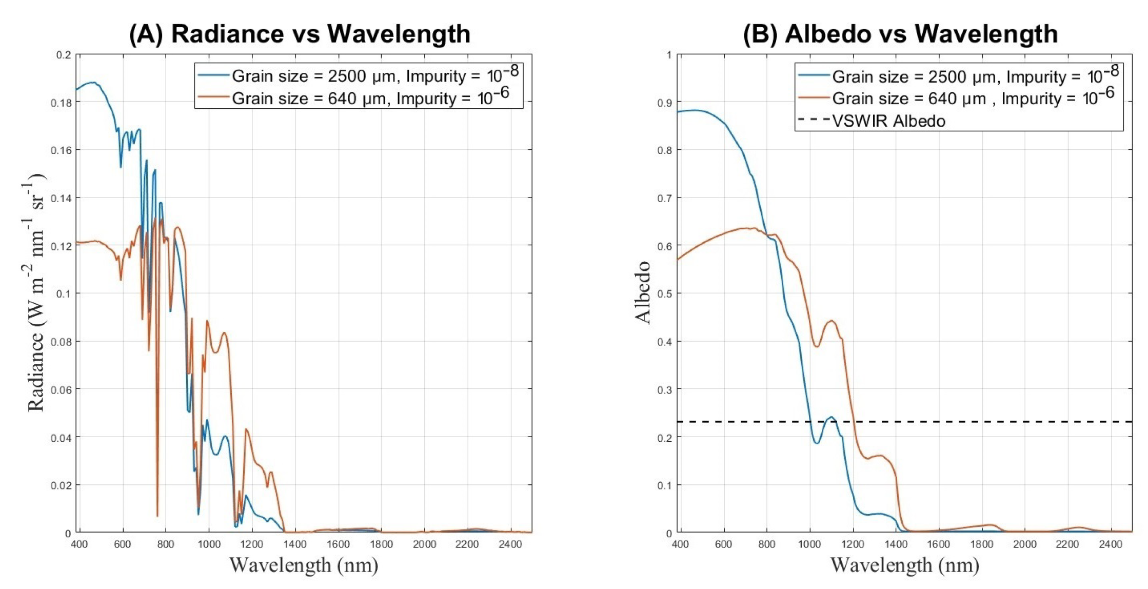
2.3.2. Illustrative Examples
3. Methods
3.1. Multi-Layer Neural Networks
3.1.1. Neural Network Setup
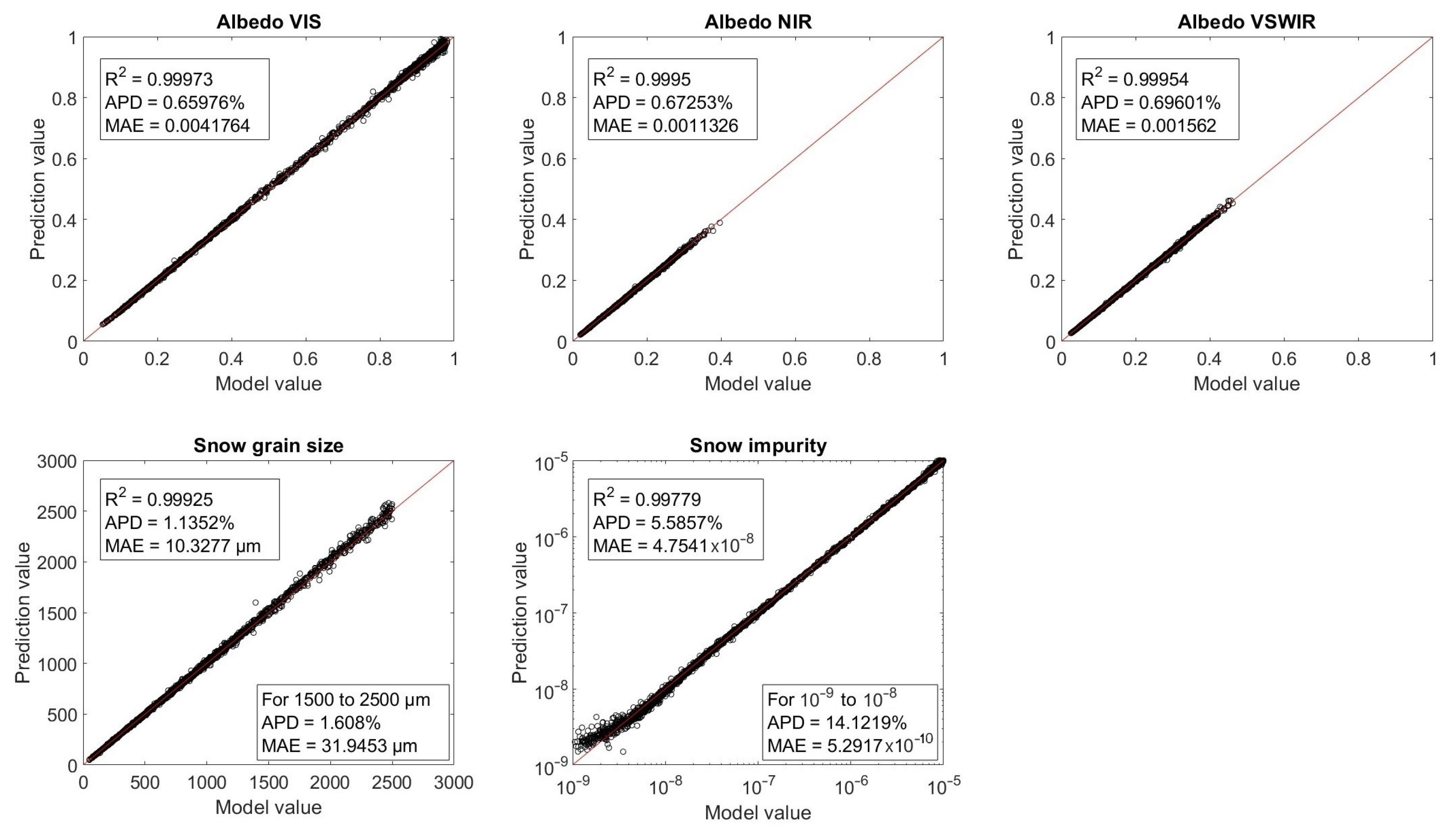
3.1.2. Training Results
3.1.3. Inversion Model
4. Results and Discussion
4.1. Results
4.2. Discussion
5. Conclusions
Author Contributions
Funding
Data Availability Statement
Conflicts of Interest
References
- Frei, A.; Tedesco, M.; Lee, S.; Foster, J.; Hall, D.; Kelly, R.; Robinson, D. A review of global satellite-derived snow products. Adv. Space Res. 2012, 50, 1007–1029. [Google Scholar] [CrossRef]
- Deltz, A.; Kruenzer, C.; Gessner, U.; Dech, S. Remote sensing of snow—A review of available methods. Int. J. Remote Sens. 2012, 33, 4094–4134. [Google Scholar]
- Tedesco, M. Remote Sensing of the Cryosphere; Wiley: New York, NY, USA, 2015. [Google Scholar]
- Stamnes, K.; Li, W.; Eide, H.; Aoki, T.; Hori, M.; Storvold, R. ADEOS-II/GLI snow/ice products: Part I-Scientific basis. Remote Sens. Environ. 2007, 111, 258–273. [Google Scholar] [CrossRef]
- Lyapustin, A.; Tedesco, M.; Wang, Y.; Aoki, T.; Hori, M.; Kokhanovsky, A. Retrieval of snow grain size over greenland from modis. Remote Sens. Environ. 2009, 113, 1976–1987. [Google Scholar] [CrossRef]
- Zege, E.; Katsev, I.; Malinka, A.; Prikhach, A.; Heygster, G.; Wiebe, H. Algorithm for retrieval of the effective snow grain size and pollution amount from satellite measurements. Remote Sens. Environ. 2011, 115, 2674–2685. [Google Scholar] [CrossRef]
- Kokhanovsky, A.; Lamare, M.; Danne, O.; Brockmann, C.; Dumont, M.; Brockmann, C.; Picard, G.; Arnaud, L.; Favier, V.; Jourdain, B.; et al. Retrieval of snow properties from the sentinel-3 ocean and land colour instrument. Remote Sens. 2019, 11, 2280. [Google Scholar] [CrossRef]
- Cawse-Nicholson, K.; Townsend, P.A.; Schimel, D.; Assiri, A.M.; Blake, P.L.; Buongiorno, M.F.; Campbell, P.; Carmon, N.; Casey, K.A.; Correa-Pabó, R.E.; et al. NASA’s surface biology and geology designated observable: A perspective on surface imaging algorithms. Remote Sens. Environ. 2021, 257, 112349. [Google Scholar] [CrossRef]
- National Academies of Sciences Engineering Medicine. Thriving on Our Changing Planet: A Decadal Strategy for Earth Observation from Space; The National Academies Press: Washington, DC, USA, 2018. [Google Scholar]
- Rittger, K.; Painter, T.; Dozier, J. Assessment of methods for mapping snow cover from MODIS. Adv. Water Resour. 2013, 51, 367–380. [Google Scholar] [CrossRef]
- Kokhanovsky, T.; Shimada, R.; Aoki, T.; Hori, M. The determination of snow parameters using SGLI/GCOM-C spaceborne top-of-atmosphere spectral reflectance measurements over Antarcticar. J. Quant. Spectrosc. Radiat. Transf. 2022, 287, 108226. [Google Scholar] [CrossRef]
- Hori, M.; Sugiura, K.; Kobayashi, K.; Aoki, T.; Tanikawa, T.; Kuchiki, K.; Niwano, M.; Enomoto, H. A 38-year (1978–2015) Northern Hemisphere daily snow cover extent product derived using consistent objective criteria from satellite-borne optical sensors. Remote Sens. Environ. 2017, 191, 402–418. [Google Scholar] [CrossRef]
- Thompson, D.; Natraj, V.; Green, R.; Helmlinger, M.; Gao, B.; Eastwood, M. Optimal estimation for imaging spectrometer atmospheric correction. Remote Sens. Environ. 2018, 216, 355–373. [Google Scholar] [CrossRef]
- Painter, T.; Seidel, F.; Bryant, A.; Skiles, S.; Rittger, K. Imaging spectroscopy of albedo and radiative forcing by light-absorbing impurities in mountain snow. J. Geophys. Res.-Atmos. 2013, 118, 9511–9523. [Google Scholar] [CrossRef]
- Gubler, H. Model of dry snow metamorphism by interparticle vapor flux. J. Geophys. Res. 1985, 90, 8081–8092. [Google Scholar] [CrossRef]
- Langham, E. Physics and properties of snowcover. In Handbook of Snow, Principles, Processes, Management and Use; Pergamon Press: Oxford, UK, 1981; pp. 275–337. [Google Scholar]
- Male, D.; Gray, D. Snowcover ablation and runoff. In Handbook of Snow, Principles, Processes, Management and Use; Pergamon Press: Oxford, UK, 1981; pp. 360–436. [Google Scholar]
- Palm, E.; Tveitereid, M. On heat and mass flow through dry snow. J. Geophys. Res. 1979, 84, 745–749. [Google Scholar] [CrossRef]
- Colbeck, S. Theory of metamorphism of dry snow. J. Geophys. Res. 1983, 88, 5475–5482. [Google Scholar] [CrossRef]
- Budd, W.; Dingle, W.; Radok, U. The Byrd snow drift project: Outline and basic results. Stud. Antarct. Meteorol. Am. Geophys. Union Antarct. Res. Ser. 1966, 9, 71–134. [Google Scholar]
- Schmidt, R.; Troendle, C. Sublimation of intercepted snow as a global source of water vapour. In Proceedings of the 60th Annual Western Snow Conference, Jackson Hole, WY, USA, 14–16 April 1992; pp. 1–9. [Google Scholar]
- Marsh, P.; Woo, M. Wetting front advance and freezing of meltwater within a snowcover 1. Observations in the Canadian Arctic. Water Resources Res. 1984, 20, 1853–1864. [Google Scholar] [CrossRef]
- Laszlo, I.; Liu, H.; Kim, H.Y.; Pinker, R.T. Chapter 15-Shortwave Radiation from ABI on the GOES-R Series; The GOES-R Series; Goodman, S.J., Schmit, T.J., Daniels, J., Redmon, R.J., Eds.; Elsevier: Amsterdam, The Netherlands, 2020; pp. 179–191. [Google Scholar]
- Wiscombe, W.; Warren, S. A Model for the Spectral Albedo of Snow. I: Pure Snow. J. Atmos. Sci. 1980, 37, 2712–2733. [Google Scholar] [CrossRef]
- Warren, S.; Wiscombe, W. A Model for the Spectral Albedo of Snow. II: Snow Containing Atmospheric Aerosols. J. Atmos. Sci. 1980, 37, 2734–2745. [Google Scholar] [CrossRef]
- O’Neil, A.; Gray, D. Spatial and temporal variations of the albedo of a prairie snowpack. In The Role of Snow and Ice in Hydrology: Proceedings of the Bang Symposium; Unesco-WMO-IAHS: Paris, France, 1973; pp. 176–186. [Google Scholar]
- Stamnes, K.; Hamre, B.; Stamnes, S.; Chen, N.; Fan, Y.; Li, W.; Lin, Z.; Stamnes, J. Progress in forward-inverse modeling based on radiative transfer tools for coupled atmosphere-snow/ice-ocean systems: A review and description of the AccuRT model. Appl. Sci. 2018, 8, 2682. [Google Scholar] [CrossRef]
- Wang, W.; Dungan, J.; Genovese, V.; Shinozuka, Y.; Yang, Q.; Liu, X.; Poulter, B.; Brosnan, I. Development of the Ames Global Hyperspectral Synthetic Data Set: Surface Bidirectional Reflectance Distribution Function. J. Geophys. Res. Biogeosci. 2023, 128, e2022JG007363. [Google Scholar] [CrossRef]
- Thuillier, G.; Herse, M.; Labs, D.; Foujols, T.; Peetermans, W.; Gillotay, D.; Simon, P.; Mandel, H. The Solar Spectral Irradiance from 200 to 2400 nm as Measured by the SOLSPEC Spectrometer from the Atlas and Eureca Missions. Sol. Phys. 2003, 214, 1–22. [Google Scholar] [CrossRef]
- Anderson, G.; Chetwynd, J.; Wang, J.; Hall, L.; Kneizys, F.; Kimball, L.; Bernstein, L.; Acharya, P.; Berk, A.; Robertson, D.; et al. MODTRAN 3: Suitability as a flux-divergence code. In Proceedings of the 4th ARM Science Team Meeting, Charleston, SC, USA, 28 February–3 March 1994; pp. 75–80. [Google Scholar]
- ATSM Standard G173-03; Standard Tables for Reference Solar Spectral Irradiances: Direct Normal and Hemispherical on 37° Tilted Surface. ASTM International: West Conshohocken, PA, USA, 2020; Volume 114, pp. 1–21.
- Anderson, G.; Clough, S.; Kneizys, F.; Chetwynd, J.; Shettle, E. AFGL Atmospheric Constituent Profiles (0–120 km); AFGL-TR-86-0110; Air Force Geophysics Laboratory: Hanscom, MA, USA, 1986; p. 01736. [Google Scholar]
- Kassianov, E.; Cromwell, E.; Monroe, J.; Riihimaki, L.; Flynn, C.; Barnard, J.; Michalsky, J.J.; Hodges, G.; Shi, Y.; Comstock, J.M. Harmonized and high-quality datasets of aerosol optical depth at a US continental site, 1997–2018. Sci. Data 2021, 8, 82. [Google Scholar] [CrossRef] [PubMed]
- Stamnes, K.; Hamre, B.; Stamnes, J.; Ryzhikov, G.; Birylina, M.; Mahoney, R.; Hauss, B.; Sei, A. Modeling of radiation transport in coupled atmosphere-snow-ice-ocean systems. J. Quant. Spectrosc. Radiat. Transf. 2011, 112, 714–726. [Google Scholar] [CrossRef]
- Grenfell, T.; Warren, S.; Mullen, P. Reflection of solar radiation by the Antarctic snow surface at ultraviolet, visible, and near-infrared wavelengths. J. Geophys. Res. 1994, 99, 669–684. [Google Scholar] [CrossRef]
- Chen, S.; Billings, S.; Grant, P. Non-linear system identification using neural networks. Int. J. Control 1990, 51, 1191–1214. [Google Scholar] [CrossRef]
- D’Alimonte, D.; Zibordi, G. Phytoplankton determination in an optically complex coastal region using a multilayer perceptron neural network. IEEE Trans. Geosci. Remote Sens. 2003, 41, 2861–2868. [Google Scholar] [CrossRef]
- Fan, Y.; Li, W.; Chen, N.; Ahn, J.; Park, Y.; Kratzer, S.; Schroeder, T.; Ishizaka, J.; Chang, R.; Stamnes, K. OC-SMART: A machine learning based data analysis platform for satellite ocean color sensors. Remote Sens. Environ. 2021, 253, 112236. [Google Scholar] [CrossRef]
- Jiang, T.; Gradus, J.; Rosellini, A. Supervised Machine Learning: A Brief Primer. Behav. Ther. 2020, 51, 675–687. [Google Scholar] [CrossRef]
- Mayer, N.; Ilg, E.; Fischer, P.; Hazirbas, C.; Cremers, D.; Dosovitskiy, A.; Brox, T. What Makes Good Synthetic Training Data for Learning Disparity and Optical Flow Estimation? CoRR 2018, 126, 942–960. [Google Scholar] [CrossRef]
- Diederik, P.; Ba, J. Adam: A Method for Stochastic Optimization. arXiv 2015, arXiv:1412.6980. [Google Scholar]


| Parameter | Data Range | Distribution | Mean |
|---|---|---|---|
| Relative azimuth angle | 0 to 180 (degrees) | Uniform | 89.87 |
| Viewing zenith angle | 0 to 45 (degrees) | Uniform | 22.55 |
| Solar zenith angle | 20 to 75 (degrees) | Uniform | 47.62 |
| Snow grain size | 50 to 2500 (µm) | Log-normal | 835 µm |
| Snow impurity concentration | to (ratio) | Log-normal |
| SBG Algorithm | Score | APD | MAE |
| Albedo VIS | 0.999 | 0.660 % | 0.004 |
| Albedo NIR | 0.999 | 0.673 % | 0.001 |
| Albedo VSWIR | 0.999 | 0.670 % | 0.002 |
| Snow grain size | 0.999 | 1.135 % | 10.33 µm |
| Snow impurity | 0.998 | 5.586 % | 4.754 |
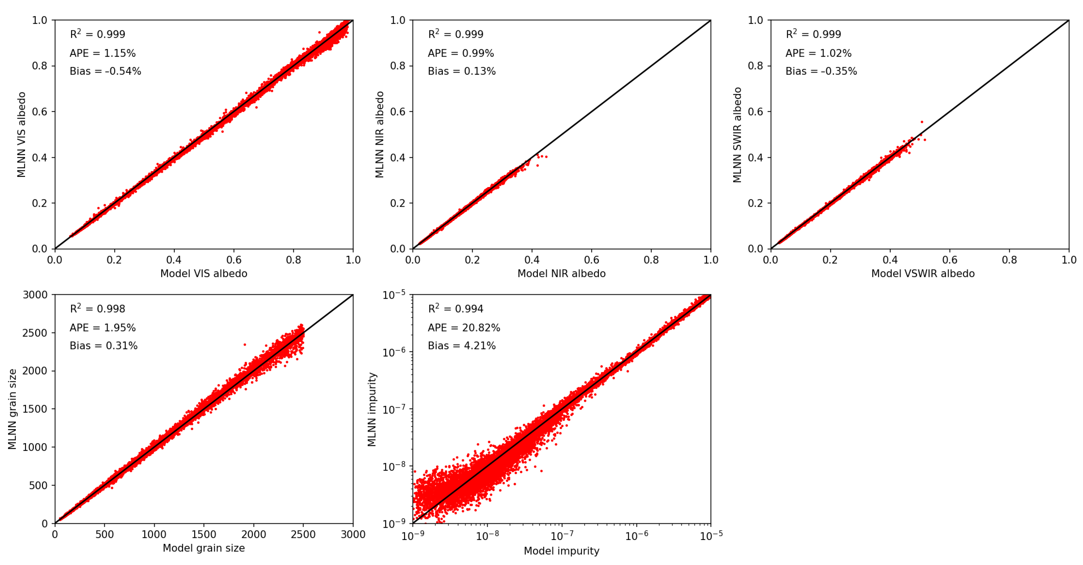
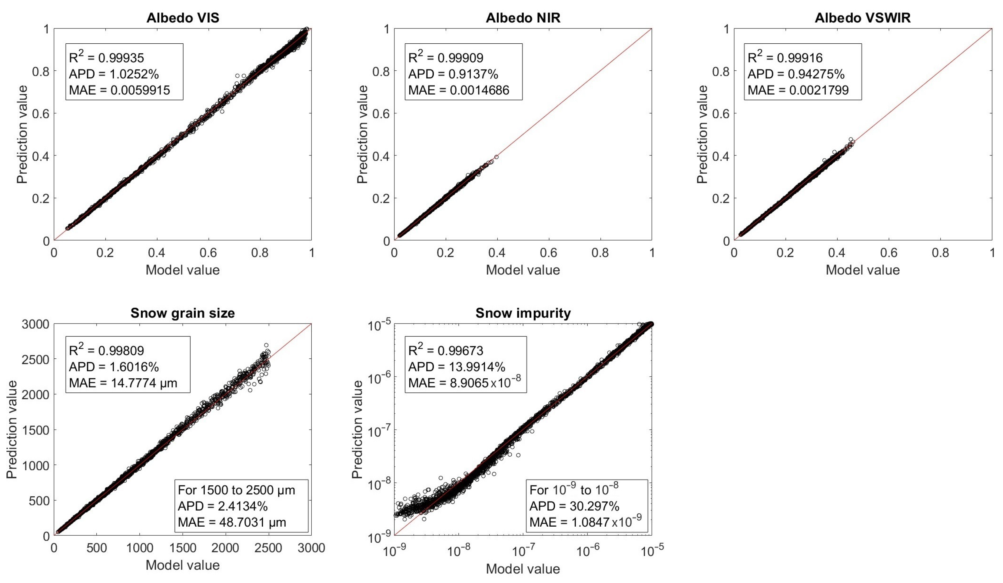
| MODIS algorithm | Score | APD | MAE |
| Albedo VIS | 0.999 | 1.025 % | 0.006 |
| Albedo NIR | 0.999 | 0.914 % | 0.001 |
| Albedo VSWIR | 0.999 | 0.943 % | 0.002 |
| Snow grain size | 0.998 | 1.602 % | 14.78 µm |
| Snow impurity | 0.997 | 13.99 % | 8.907 |
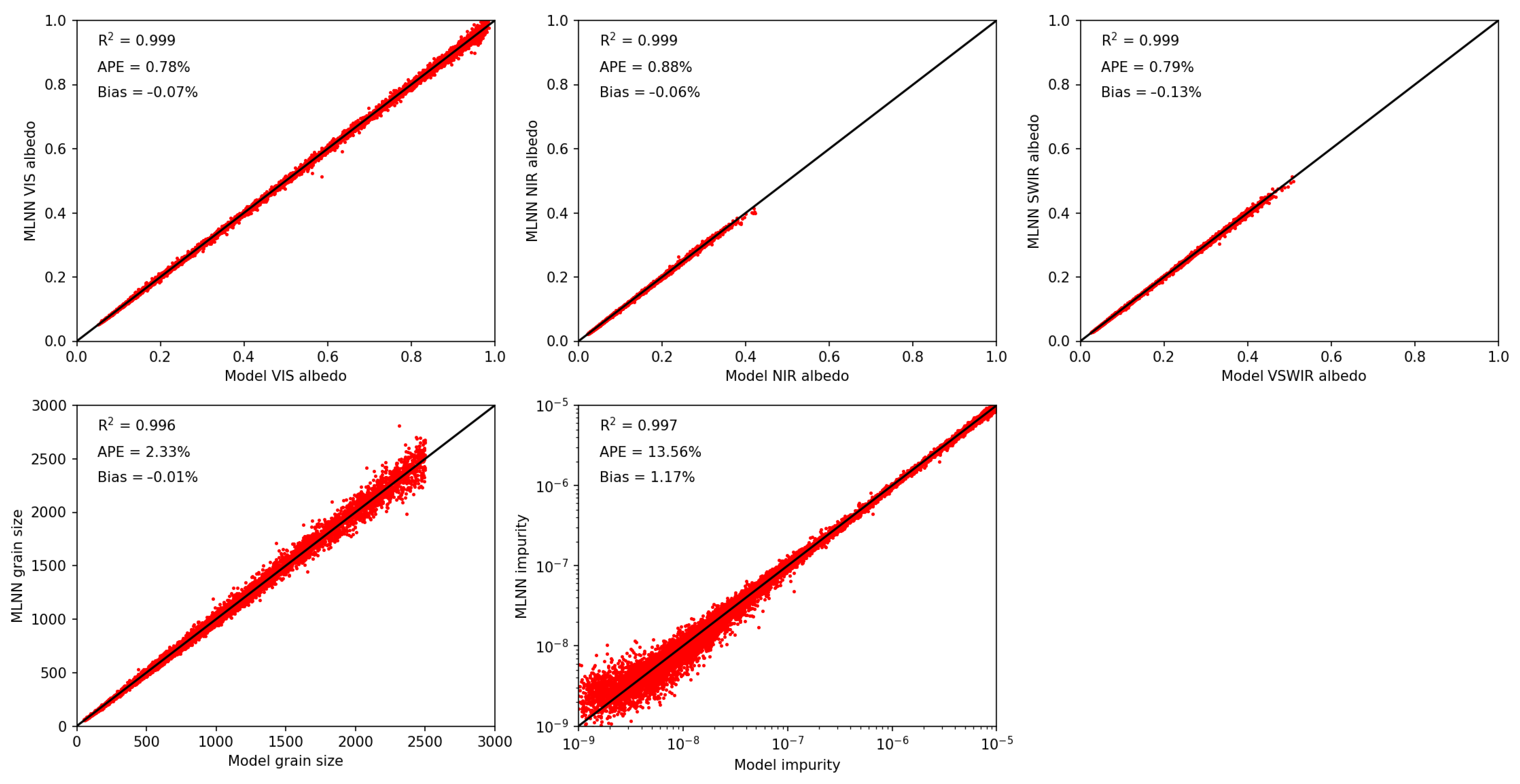
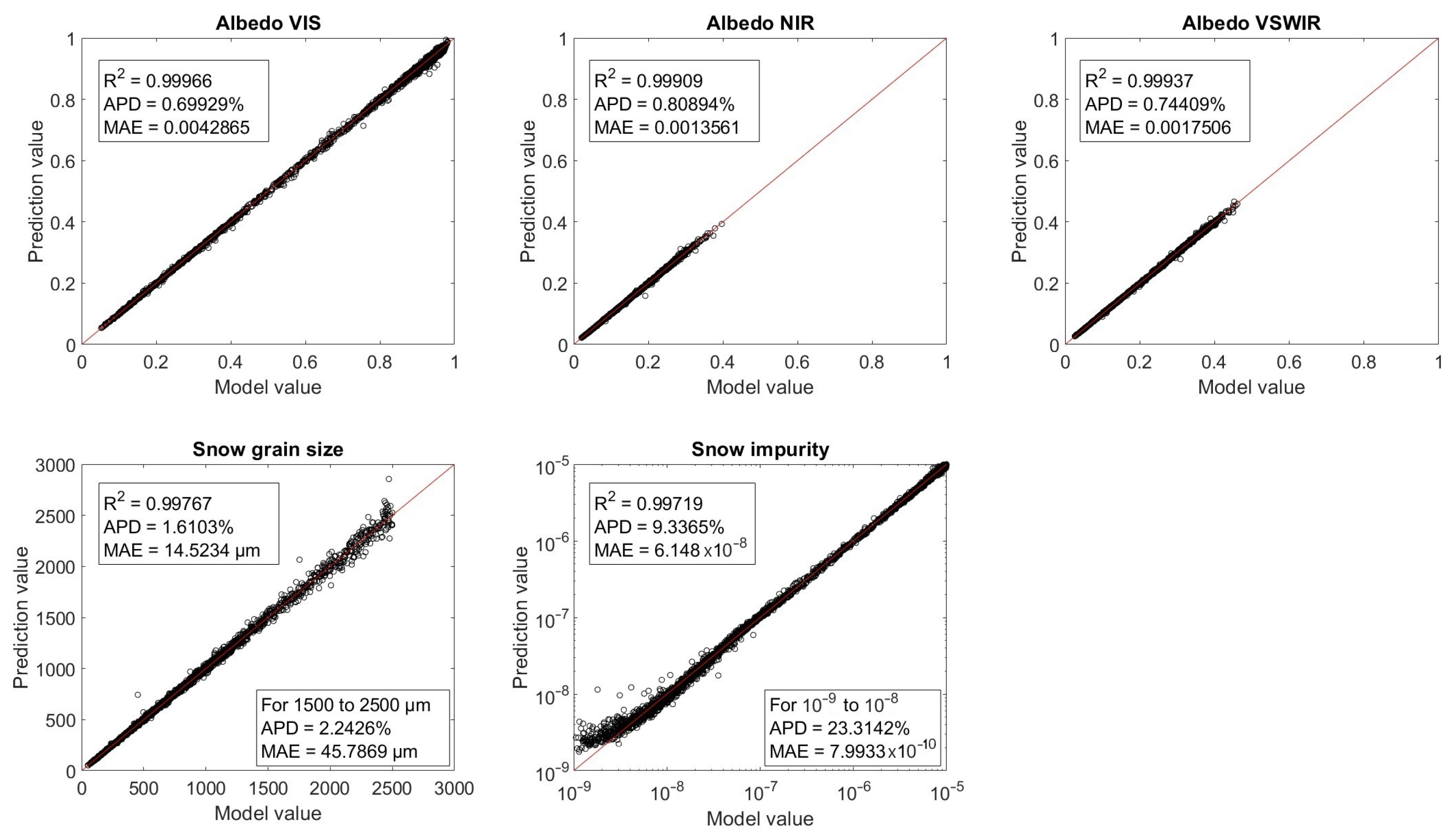
| SGLI algorithm | Score | APD | MAE |
| Albedo VIS | 0.999 | 0.699 % | 0.004 |
| Albedo NIR | 0.999 | 0.809 % | 0.001 |
| Albedo VSWIR | 0.999 | 0.744 % | 0.002 |
| Snow grain size | 0.998 | 1.610 % | 14.52 µm |
| Snow impurity | 0.997 | 9.34 % | 6.148 |
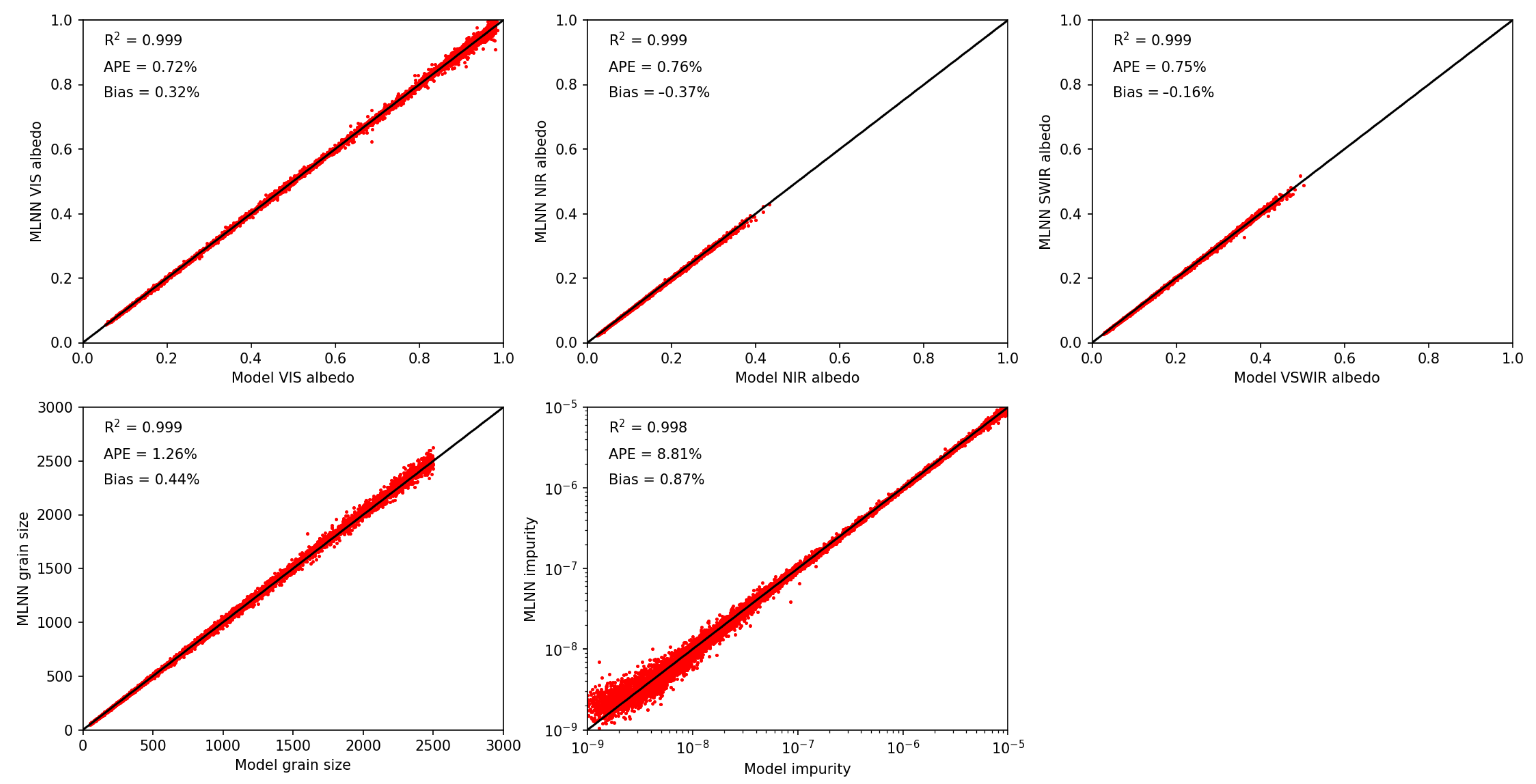
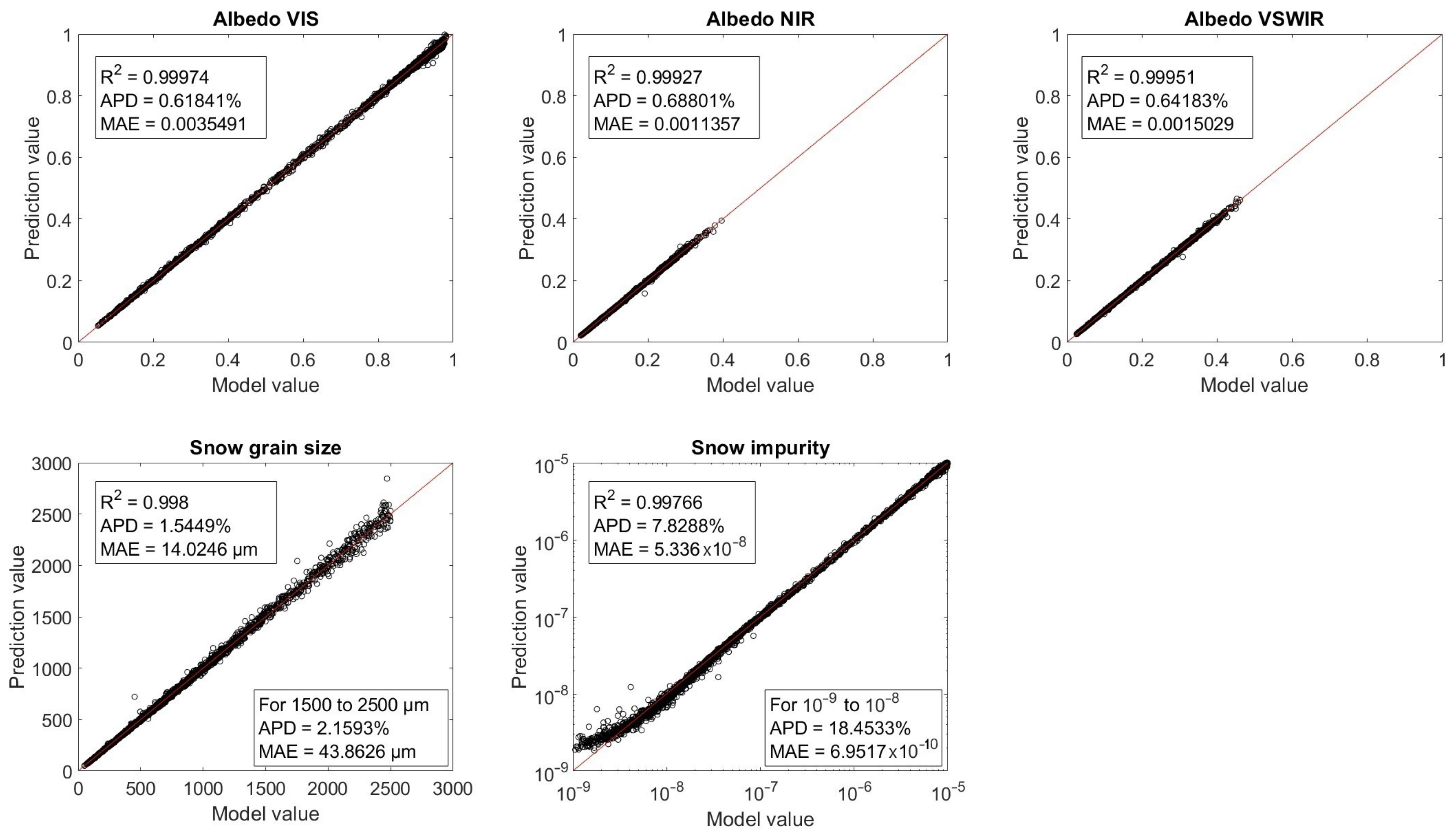
| Max-Min algorithm | Score | APD | MAE |
| Albedo VIS | 0.999 | 0.618 % | 0.004 |
| Albedo NIR | 0.999 | 0.688 % | 0.001 |
| Albedo VSWIR | 0.999 | 0.641 % | 0.002 |
| Snow grain size | 0.998 | 1.545 % | 14.02 µm |
| Snow impurity | 0.998 | 7.829 % | 5.336 |
Disclaimer/Publisher’s Note: The statements, opinions and data contained in all publications are solely those of the individual author(s) and contributor(s) and not of MDPI and/or the editor(s). MDPI and/or the editor(s) disclaim responsibility for any injury to people or property resulting from any ideas, methods, instructions or products referred to in the content. |
© 2023 by the authors. Licensee MDPI, Basel, Switzerland. This article is an open access article distributed under the terms and conditions of the Creative Commons Attribution (CC BY) license (https://creativecommons.org/licenses/by/4.0/).
Share and Cite
Pachniak, E.; Li, W.; Tanikawa, T.; Gatebe, C.; Stamnes, K. Remote Sensing of Snow Parameters: A Sensitivity Study of Retrieval Performance Based on Hyperspectral versus Multispectral Data. Algorithms 2023, 16, 493. https://doi.org/10.3390/a16100493
Pachniak E, Li W, Tanikawa T, Gatebe C, Stamnes K. Remote Sensing of Snow Parameters: A Sensitivity Study of Retrieval Performance Based on Hyperspectral versus Multispectral Data. Algorithms. 2023; 16(10):493. https://doi.org/10.3390/a16100493
Chicago/Turabian StylePachniak, Elliot, Wei Li, Tomonori Tanikawa, Charles Gatebe, and Knut Stamnes. 2023. "Remote Sensing of Snow Parameters: A Sensitivity Study of Retrieval Performance Based on Hyperspectral versus Multispectral Data" Algorithms 16, no. 10: 493. https://doi.org/10.3390/a16100493
APA StylePachniak, E., Li, W., Tanikawa, T., Gatebe, C., & Stamnes, K. (2023). Remote Sensing of Snow Parameters: A Sensitivity Study of Retrieval Performance Based on Hyperspectral versus Multispectral Data. Algorithms, 16(10), 493. https://doi.org/10.3390/a16100493