Predicting Dissolution Kinetics of Tricalcium Silicate Using Deep Learning and Analytical Models

Abstract

The dissolution kinetics of Portland cement is a critical factor in controlling the hydration reaction and improving the performance of concrete. Tricalcium silicate (C₃S), the primary phase in Portland cement, is known to have complex dissolution mechanisms that involve multiple reactions and changes to particle surfaces. As a result, current analytical models are unable to accurately predict the dissolution kinetics of C₃S in various solvents when it is undersaturated with respect to the solvent. This paper employs the deep forest (DF) model to predict the dissolution rate of C₃S in the undersaturated solvent. The DF model takes into account several variables, including the measurement method (i.e., reactor connected to inductive coupled plasma spectrometer and flow chamber with vertical scanning interferometry), temperature, and physicochemical properties of solvents. Next, the DF model evaluates the influence of each variable on the dissolution rate of C₃S, and this information is used to develop a closed-form analytical model that can predict the dissolution rate of C₃S. The coefficients and constant of the analytical model are optimized in two scenarios: generic and alkaline solvents. The results show that both the DF and analytical models are able to produce reliable predictions of the dissolution rate of C₃S when it is undersaturated and far from equilibrium.

1. Introduction

Portland cement (PC) is the fundamental material for modern infrastructure, but its production contributes significantly to global CO₂ emissions, accounting for about 9% of total emissions [1,2,3]. To improve the sustainability and performance of PC, it is important to understand the hydration reaction of its primary component, tricalcium silicate (C₃S). C₃S is the most abundant component in PC, making up more than 50% of its composition [4,5,6]. When C₃S reacts with water, it undergoes a series of chemical reactions that result in the dissolution of calcium and silicate ions, followed by the formation of calcium silicate hydrate and portlandite [4]. While the phase transformations that occur at later stages of the hydration are well documented [4,7], the dissolution kinetics of C₃S at early stages remains a controversial subject. However, it is important to understand the dissolution kinetics of C₃S when it is undersaturated with respect to solvent. The undersaturation of C₃S solution presents the initial and induction periods of cement hydration [4,6]. The dissolution mechanisms of C₃S are different when the solution is in undersaturation and saturation (i.e., hydration products form) [6,8]. By studying the dissolution behaviors of C₃S, we can gain a better understanding of the factors that affect the hydration kinetics of cement. This knowledge can be used to develop novel cement formulations and improve cement performance.

Despite many studies that have sought to uncover the mechanisms (e.g., protective phase [9,10,11] and double layer theory [12]) behind the dissolution of C₃S and minerals in recent decades, a definitive rate-controlling mechanism remains elusive due to the complex interaction of physicochemical parameters between solids and aqueous solvents. The most widely accepted theory to explain the dissolution kinetics of C₃S and minerals is the inverse crystal nucleation theory [6,13,14]. This theory posits that, similar to the process of crystal growth, the dissolution of C₃S and minerals is primarily determined by the density of pre-existing steps on the surface of minerals [14]. These steps are formed by dislocation defects and the nucleation of two-dimensional vacancy islands at impurities or homogenous sites. The growth of vacancy islands on a surface is determined by the Gibbs–Thomson effect, a thermodynamic principle that dictates their critical size [15,16]. If a vacancy exceeds this critical size, it will continue to grow. At the critical size, the free energy change reaches a maximum, creating an energy barrier that must be overcome for vacancy growth to continue. The energy barriers that must be overcome by the vacancy islands have a proportional relationship with the interfacial energy, but an inverse relationship with the degree of undersaturation [15,16]. While the solution is near the equilibrium, the density of steps of the solid is dominated by dislocation defects, as the energy barriers are too high for vacancy islands to overcome.

Except for surface defects, other experimental parameters—for example, solvent chemistry [8,17], surface geometry [18,19,20,21,22,23], and mineral composition [24,25,26]—also substantially influence the dissolution kinetics of C₃S and minerals. By incorporating these parameters into analytical models, it is possible to reveal underlying structures between dissolution kinetics and physicochemical properties of minerals and solvents. The following review focuses on existing analytical models (shown in Table 1) that have been used to predict the dissolution kinetics of C₃S and minerals. Some of these models have been successful in accurately predicting the dissolution kinetics of minerals. The symbols used in these models are defined as follows: $\mathrm{\Delta }{G}_r$ is the Gibbs free energy of the overall reaction; T is the temperature; R is the gas constant; A is the effective surface area of material; a_i is the ion activity of species i; E_a is the activation energy; n, n_i, k, and k_i are constants; and g(I) is the function of ionic strength.

The analytical model developed by Burch et al. [27] is based on the transition state theory and the Burton–Cabrera–Frank theory. It shows that the dissolution rate of a mineral depends exponentially on the Gibbs free energy of the overall dissolution and the temperature. However, this model cannot accurately predict the dissolution kinetics of a solid–solvent system that is near the equilibrium. This is because the model does not account for the transition from step retreat to dislocation-controlled dissolution. The model developed by Lasaga et al. [28] accounts for various factors such as surface area, temperature, ionic strength, H⁺ concentration in the solvent, and the change in Gibbs free energy related to dissolution. This model is widely used in the cement community to predict the dissolution kinetics of C₃S [6]. In addition to modeling from a thermodynamic perspective, several studies [29,30,31,32,33] have explained the dissolution kinetics of minerals using the ion leaching theory. Strachan’s model [29] accounts for both H⁺ and OH⁻ in the leaching process, as these ions leach species from mineral surfaces with different activation energies. Other studies [32,33,34,35,36] have found that cations (excluding H⁺) in solvents can also contribute to mineral surface leaching. Oelkers et al. [32] have emphasized the role of the ion activity ratio of H⁺ to cations in mineral dissolution kinetics. This model divides the process into two scenarios: if the ion activity ratio is small, a large number of cations remain on the material surface, which dominates the leaching and dissolution processes; if the ratio is large, the dissolution rate is independent of cations. This model has been used to predict the dissolution kinetics of various minerals [33].

Table 1. Summary of current dissolution kinetics models for C₃S and minerals.

$Rate=k_1\left[1-\exp \left(-n{\left(\frac{\mathrm{\Delta }{G}_r}{RT}\right)}^{n_1}\right)\right]+k_2{\left[1-\exp \left(-\frac{\mathrm{\Delta }{G}_r}{RT}\right)\right]}^{n_2}$	Burch et al. [27]
$Rate=k_0·A_{min}·\exp \left(-\frac{E_a}{RT}\right)·a_{H+}^{nH+}·{\displaystyle \prod }_i{a}_i^{ni}·g\left(I\right)·f\left(\mathrm{\Delta }{G}_r\right)$	Lasaga et al. [28]
$Rate=k\left[a_{H+}^{n_{OH-}}+a_{OH-}^{n_{OH-}}\right]$	Strachan [29]
$Rate=k{\displaystyle \prod }_{i=1,i\ne k}^i\left[\frac{k_i{\left(\frac{a_{H+}^{Vi}}{a_{Mi}^{Vi}}\right)}^n}{1+k_i{\left(\frac{a_{H+}^{Vi}}{a_{Mi}^{Vi}}\right)}^n}\right]$	Oelkers et al. [32]

Table 1. Summary of current dissolution kinetics models for C₃S and minerals.

$Rate=k_1\left[1-\exp \left(-n{\left(\frac{\mathrm{\Delta }{G}_r}{RT}\right)}^{n_1}\right)\right]+k_2{\left[1-\exp \left(-\frac{\mathrm{\Delta }{G}_r}{RT}\right)\right]}^{n_2}$	Burch et al. [27]
$Rate=k_0·A_{min}·\exp \left(-\frac{E_a}{RT}\right)·a_{H+}^{nH+}·{\displaystyle \prod }_i{a}_i^{ni}·g\left(I\right)·f\left(\mathrm{\Delta }{G}_r\right)$	Lasaga et al. [28]
$Rate=k\left[a_{H+}^{n_{OH-}}+a_{OH-}^{n_{OH-}}\right]$	Strachan [29]
$Rate=k{\displaystyle \prod }_{i=1,i\ne k}^i\left[\frac{k_i{\left(\frac{a_{H+}^{Vi}}{a_{Mi}^{Vi}}\right)}^n}{1+k_i{\left(\frac{a_{H+}^{Vi}}{a_{Mi}^{Vi}}\right)}^n}\right]$	Oelkers et al. [32]

Although previous studies have proposed various models for predicting dissolution kinetics of minerals based on disparate theories, none of these models can predict the dissolution kinetics of C₃S in a high-fidelity manner with a coefficient of determination (R²) above 0.90. This is because there are several knowledge gaps in the state-of-the-art analytical models. First, it is not possible to account for all the influential variables (e.g., ions in the solvent; physicochemical properties of C₃S particles; temperature; etc.) in a single analytical model. Moreover, it is difficult to incorporate a variable into analytical models without a clear understanding of its role in the dissolution process. Next, coefficients are not generic, thus requiring additional calibration while applying the model to a new C₃S-solvent systems. Lastly, some parameters (e.g., ion activity; Gibbs free energy; activation energy; etc.) are obtained from additional quantitative and qualitative analyses of experimental results, which makes the model difficult to use and increases the likelihood of human error.

Measuring the dissolution rate of C₃S is a challenge because the solubility of calcium silicate hydrate is much lower than that of C₃S, which means calcium silicate hydrate will precipitate before C₃S completely dissolves, unless a very small amount of C₃S is used. As a result, only a few studies have attempted to measure the C₃S dissolution rate. Those studies have applied two different methods to measure the dissolution rate of C₃S: reactor connected to inductive coupled plasma (ICP) spectrometer [37,38]; and flow chamber with vertical scanning interferometry (VSI) [39]. In the first method, C₃S particles dissolve into the solvent in a reactor, and the ICP spectrometer measures ion concentrations of the solution for the first couple of minutes to determine the dissolution rate. The change in C₃S surface area can be ignored because of the short measurement duration. In the second method, the solvent is flushed over the surface of the C₃S bulk for a period of time, and the VSI is used to measure the leaching depth and determine the dissolution rate. Because these two methods are based on different experimental principles and use different parameters, a single analytical model cannot be used to predict the dissolution rate from both methods.

Machine learning (ML), a data-driven framework, has been employed in many studies [40,41,42,43,44,45,46,47,48,49,50] to predict properties for multi-component systems (e.g., cement, glass, and biomaterials) in a high-fidelity manner. ML models acquire knowledge of underlying input-output correlations (all possible correlations can be included) from a training dataset, and subsequently utilize such knowledge to produce predictions for new mixture designs, without requiring an understanding of the mechanisms behind the materials. Elçiçek et al. [49] have successfully employed an artificial neural network to discover the underlying structure between the dissolution kinetics of colemanite, a type of boron mineral, in complex dissolution environments. A decision-tree-based ensemble model has demonstrated remarkable performance, in terms of R² ≈ 0.98, on predictions of dissolution rate for bioactive glasses in various pH environments [40]. ML models incorporating topological constraints of glasses have been employed to predict and extrapolate dissolution kinetics of silicate glasses without violating fundamental material laws [43]. Although extensive studies have applied ML methods to predictions of material dissolution kinetics, there is currently no literature that shows that an ML model is a valid approach to predict the dissolution rate of C₃S when it is undersaturated with respect to the solvent.

In this study, a deep forest (DF) model is trained using a heterogenous database of C₃S dissolution rate measured by the reactor connected to ICP spectrometer and flow chamber with VSI methods. The rigorously trained model produces high-fidelity, a priori predictions of the C₃S dissolution rate. It is notable that ML models can predict the hydration kinetics of PC at any given age, which has been shown in our previous studies [51,52,53]. This study only focuses on the dissolution kinetics at the initial period (i.e., undersaturated solution) because the hydration products precipitate and cause the solution to reach saturation after a short time of the dissolution of C₃S. Then, the influence of each input variable on the dissolution rate is evaluated, and this knowledge is used to develop a simple, closed-form analytical model based on fundamental thermodynamic and kinetic frameworks, such as ion activity, ion strength, and ion activity product (IAP). The analytical model reveals fundamental correlations behind the C₃S dissolution process, which are the critical information that cannot be provided by ML models due to their “black-box” nature. Furthermore, the analytical model can be used by all end users, regardless of their background or of their access to ML models. Overall, this study is the first to develop an ML model to predict with high fidelity the dissolution kinetics of C₃S dissolved in various solvents when it is undersaturated and far from equilibrium.

2. Database Collection

The C₃S dissolution database used in this study consists of 292 data records, which were consolidated from Nicoleau et al. [37,38] and Juilland and Gallucci [39]. However, these data records are not compatible with our database due to differences in experimental parameters. For example, Bellmann et al. [54] measured the dissolution rate of C₃S at the induction period and later ages; Damidot et al. [55] and Barret et al. [56] used the filter dissolution technique; and Robin et al. [57] used the face-specific dissolution method to measure the dissolution rate of C₃S. The database used in this study contains 11 input parameters: temperature (°C); specific surface area (SSA) of C₃S (m²/g); flow rate (mL/min/mm²) initial concentration of Na, Cl, Ca, Si, Cs, K, and SO₄ (mM); and initial pH (unitless). The output is the dissolution rate of C₃S (µmol/m²/s). There are 92 data-records from Nicoleau et al. [37,38] measured by the reactor connected to ICP spectrometer method. Since the flow rate is not applicable in this method, it was set as 0. Several solvents with different ions were utilized in the reactor connected to ICP spectrometer method. There were 200 data records from Juilland and Gallucci [39] measured with the flow chamber with VSI method. Moreover, since the SSA of C₃S is not applicable in this method, it was set as 0. The solvents only contained calcium ions at different concentration levels. Four statistical parameters associated with inputs and output of the C₃S dissolution database are summarized in

Table 2. Four statistical parameters pertaining to the 12 parameters (11 inputs and 1 output in bold) of the C₃S dissolution database. The database consists of 292 unique data records.

Attribute	Unit	Min.	Max.	Mean	Std. Dev.
Temperature	°C	10	60	21.07	5.437
SSA of C3S	m2/g	0	0.400	0.112	0.171
Flow Rate	mL/min/mm2	0	1273	79.22	201.8
Initial Na Concentration	mM	0	1000	29.19	101.5
Initial Cl Concentration	mM	0	1000	18.74	113.6
Initial Ca Concentration	mM	0	20	5.824	6.561
Initial Si Concentration	mM	0	0.876	0.006	0.062
Initial Cs Concentration	mM	0	1000	5.513	65.45
Initial K Concentration	mM	0	1000	5.513	65.45
Initial SO4 Concentration	mM	0	200	8.904	34.95
Initial pH	Unitless	6.516	13.09	10.69	2.316
C3S Dissolution rate	µmol/m2/s	0.3800	154.6	27.92	32.61

.

The ML model was trained by 219 randomly selected data records from the original database. The remaining 73 data records were used to validate the performance of the model. The prediction performance was evaluated by five statistical parameters: mean absolute error (MAE); coefficient of determination (R²); mean absolute percentage error (MAPE); Pearson correlation coefficient (R); and root mean square error (RMSE).

3. Deep Forest Model

In this study, a DF model was utilized to predict C₃S dissolution kinetics based on the physicochemical properties of C₃S and solvents. The DF model was developed based on the modified classification-and-regression tree (CART) model with a combination of bagging and random selection techniques [58,59]. The DF model grows a large number of independent trees through a recursive binary split at each node [58]. To be specific, the root node receives information from a bootstrap extracted from the training dataset, and then splits to create two child nodes. This process is repeated until the homogeneity of the child nodes cannot be improved. The tree can grow as deep as it can because none of the usual pruning or smoothing algorithms are applied. This allows the DF model to maintain diversity among trees. The DF model usually contains hundreds of independent trees. Usually, a large-size forest is required to produce reliable predictions while the database contains thousands of data-records. When a testing dataset is applied to a trained DF model, trees produce independent outputs, and subsequently a bagging algorithm averages them to derive the final output. A unique feature (i.e., two-stage randomization) allows the DF model to reduce the variance and bias errors in predictions. The first randomization is that the bootstrap randomly selects data records from the parent database. Second, at each split, several randomly selected variables, instead of all variables, are used to determine the optimal split. The randomization features ensure the decorrelation between trees. Furthermore, due to the growth of a large number of trees, errors from generalization and the likelihood of overfitting are minimized. Owing to those unique features, the DF model can effectively learn input–output correlations from complex databases. Overall, the architecture of the DF can be summarized in the following steps:

N bootstrap samples are randomly selected from the training dataset. N is equal to the number of trees. In this study, N was 200. Each bootstrap can contain ~66% [60,61,62] of the data records of the training dataset. The remaining data records are “out-of-bag” (OOB) data [58].

• Each bootstrap iteration in the DF model grows a single tree. At each split, a subset of input variables is randomly selected and used to determine the optimal split scenario. The number of leaves, or the subset size, was set to five in this study. The cost function (i.e., MAE) is used to evaluate all split scenarios, and the scenario with the minimum cost is selected. Unlike other models, the DF model allows trees to grow to their maximum size without pruning or smoothing.
• Next, the DF model produces predictions for OOB data. The DF model aggregates and averages these predictions to produce an overall OOB prediction and OOB error rate. This OOB error rate can be used to evaluate the importance of each variable in influencing the model’s output.
• Lastly, at the testing stage, the DF model averages outcomes from trees to produce predictions for a new data domain.

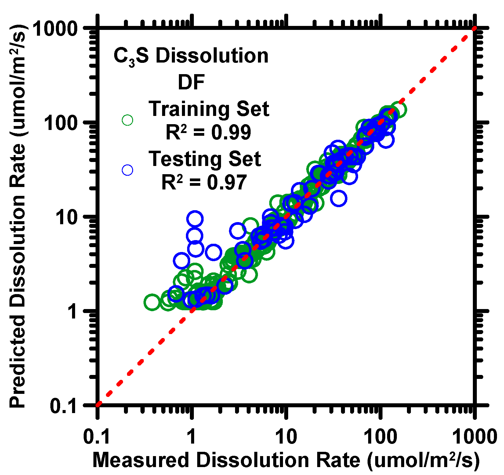
4. Predictions from Deep Forest Model

To optimize the DF model’s performance on new data records, it is crucial to meet the following criteria. First, the model requires sufficient and diverse data records to learn adequate input–output correlations (e.g., pH–dissolution rate). Second, outliers should be included in the database to ensure that the DF model comprehensively learns input–output correlations [63,64]. Herein, the outliers indicated that one or more data-records—although measured and reported properly—did not fit into the trends exhibited by the majority of the data records in the neighborhood because of some underlying (chemical, or kinetic, or thermodynamic) mechanism. Third, it is important to avoid both underfitting and overfitting to datasets. Underfitting occurs when the model is unable to learn the underlying correlations in the data, often due to a small training dataset that does not contain enough information for the model to learn from. On the other hand, overfitting occurs when the model learns local trends instead of global ones from highly similar data, resulting in poor performance on the testing dataset. To address this issue, the hyperparameters of the DF model were the 10-fold cross-validation (CV) [41,65] and grid-search methods [48,52]. These methods can help to prevent underfitting and overfitting by evaluating the model’s performance on multiple splits of the training data and using a range of different hyperparameter settings, respectively. Predictions of C₃S dissolution rate (from training and testing datasets), as produced by the DF model, are demonstrated in Figure 1. The five statistical parameters listed in

Table 3. R, R², MAE, MAPE, and RMSE evaluating prediction accuracy of the DF model against the testing dataset.

Model Name	R	R2	MAE	MAPE	RMSE
DF	Unitless	Unitless	µmol/m2/s	%	µmol/m2/s
	0.9672	0.9354	5.297	47.33	9.373

provide further evidence of the model’s performance and accuracy. Overall, by meeting the aforementioned criteria, the DF model can be trained to make highly accurate predictions on new data records.

The predicted results from the DF model for the dissolution rate of C₃S, as shown in Figure 1 and Table 3, demonstrate the model’s accuracy and reliability. The R² and RMSE values for the dissolution rate predictions were 0.94 and 9.4 µmol/m²/s, respectively, indicating a strong correlation between the predicted and measured values. In Figure 1, the predictions show a larger deviation at low dissolution rates than at high dissolution rates, but this is largely due to the use of a logarithmic scale on the y-axis. The prediction errors, as measured by the mean absolute error (MAE), were 2.01 µmol/m²/s for low dissolution rates (below 20 µmol/m²/s) and 8.67 µmol/m²/s for high dissolution rates, indicating that the DF model is able to produce reliable predictions of the dissolution rate of C₃S, regardless of the experimental method. This is a significant improvement over analytical models, which typically have a prediction accuracy of only 0.78 in terms of R² for silicate compounds [66]. The capability of the DF model to yield reliable predictions of C₃S dissolution rate is largely due to its inherent architecture [59,60,62]. First, by growing a large number (more than 100) of independent trees without smoothing or pruning, the model is able to significantly reduce the variance error in its output. Next, bias error is minimized by adopting the randomization at bootstrap and feature selections [59], which ensures that the output of one tree does not interfere with that of others. Lastly, the utilization of the 10-fold cross-validation method [65] and grid-search method [48,67] autonomously optimized the hyper-parameters so as to establish optimal input–output correlations as well as account for outliers.

The DF model can estimate the influence (in terms of importance) of input variables on the dissolution rate of C₃S. The results of this analysis are shown in Figure 2, which is organized in descending order based on the magnitude of variables’ influence. This rank is also utilized as a guide for feature selection in the development of the analytical model in Section 5.

As can be seen in Figure 2, the initial pH, Ca concentration, SSA of C₃S, and flow rate—ranked from high to low—exhibited the strongest influences on the dissolution rate of C₃S. This is expected because the Ca and OH ions (in terms of pH value) are known to be the main factors that affect the dissolution reaction according to IAP (described in Section 5) of C₃S dissolution, where a high concentration of these ions significantly reduces the dissolution rate. The SSA of C₃S is the third important variable because an increase in the interface between C₃S particles and solvent leads to a monotonical increase of the dissolution rate [20]. Similarly, the flow rate in the flow chamber with VSI method plays a significant role, as it determines the speed at which ions are leached from the surface of the C₃S particles, with higher flow rates leading to an increase in the leaching speed. Temperature is also an important variable, as previous research [27] has shown that the dissolution rate of minerals increases exponentially with an increase in temperature. Other ions in the solvent contribute less significantly to the dissolution rate. This is not a surprise, because no literature has found direct correlations between C₃S dissolution rate and those ions. Interestingly, the Si ion, one of the major ions that affect the dissolution rate of C₃S, was ranked much lower in terms of importance. This is likely because there are only three solvents in the database that contain Si ions, and the dissolution rates for these systems show little variation. As a result, the Si ions are less important than they would be in a larger and more diverse dataset. It should be noted that the importance of input variables can vary depending on the dataset used. Some variables may be found to be more important in one dataset, while being less significant in another. In this study, only a few variables were found to have a strong influence on the dissolution rate of C₃S. However, in a different dataset, different variables may exhibit a greater importance.

5. Analytical Model Development

The abovementioned results demonstrate that the DF model can produce predictions of the dissolution rate of C₃S in a high-fidelity manner. However, the use of machine learning (ML) techniques can have some limitations, such as the “black-box” issue, where the underlying input–output correlations learned by the model are difficult to interpret. Additionally, ML models may not be accessible to end users who do not have a programming background. To address these issues, this section introduces an original, closed-form analytical model that has been distilled from the DF model. This model can be used to predict the dissolution rate of C₃S and provide a better understanding of the input–output correlations involved.

The development of a reliable analytical model involves a wise selection of input variables. The inclusion of influential variables is vital to enhance the performance of the analytical model. Simultaneously, the exclusion of inconsequential variables reduces the complexity of the model. The new analytical model is developed based on Lasaga’s model [28], and some new input variables are added to it. We selected Lasaga’s model as the baseline model because it is the most used model to predict C₃S dissolution kinetics. This model accounts for the SSA of C₃S, solvent pH, temperature, and ions in solvents. The feature importance, shown in Figure 2, also confirms that those parameters dominated the dissolution rate of the C₃S. It is worth pointing out that only data from Nicoleau et al. [37,38] was employed to develop the analytical model. This is because the SSA of C₃S is not applicable in Juilland and Gallucci [39].

In the baseline model, the Gibbs free energy of the overall reaction is one of the major influential variables. To properly quantify this variable, it is important to understand the dissolution mechanism of C₃S. The dissolution process of C₃S can be considered as an inverse nucleation process [13], which is controlled by two major factors: interfacial properties and the driving force. The interfacial properties include chemical composition, chemical bond, surface defects, and impurities in crystals. Generally, the dissolution process can be divided into three steps: (1) horizontal movement at the atomic scale to form a 2D vacancy; (2) etch pit formation at dislocation; and (3) step retreat at pre-existing roughness [6,19]. The driving force of the C₃S dissolution reaction is defined as the energy to overcome the activation energy barriers for the first two steps of the dissolution process. The equation to calculate the driving force is shown in Equation (1) [6,68]:

$$\sigma =\frac{\mathrm{\Delta }\mu }{kT}=\frac{\mathrm{\Delta }{G}^{*}}{RT}=\ln \left(\frac{IAP}{K_{SP}}\right)$$

(1)

Here, $\sigma$ is the undersaturation coefficient; $\mathrm{\Delta }\mu$ is the difference in chemical potential; k is the Boltzmann constant; T is the temperature; $\mathrm{\Delta }{G}^{*}$ is the free energy difference between the undersaturated solution and the solution in equilibrium; R is the gas constant; IAP is the ion activity product to reactant species; and K_SP is the mineral solubility products. The dissolution reaction of C₃S is expressed in Equation (2) [8], and the IAP is defined in Equation (3). a_i is the ion activity of species i. The chemical equilibrium constant (K_SP) for C₃S dissolution has been estimated as 10^−17.65 [8,69].

$${\left(CaO\right)}_{3}Si{O}_2+3H_{2}O\to 3C{a}^{2+}+H_{2}Si{O}_4^{2-}+4O{H}^{-}$$

(2)

$$IAP=a_{C{a}^{2+}}^3·a_{O{H}^{-}}^4·a_{H_{2}S{O}_4^{2-}}$$

(3)

Equation (3) suggests that the value of IAP is solely determined by calcium and hydroxide ion activity. Thus, a high calcium ion activity leads to an equilibrium for the C₃S dissolution, resulting in a slower dissolution rate compared to a solvent without calcium ions [6,70]. Similarly, a basic solvent significantly decreases the dissolution rate of C₃S by containing a large amount of hydroxide ions. In this study, only H₂SiO₄²⁻ was considered in the IAP calculation because H₄SiO₄ and H₃SiO₄⁻ can deprotonate to form H₂SiO₄²⁻ [71,72]. To clearly observe the influence of IAP on dissolution rate, Figure 3 shows the correlation between the degree of undersaturation (IAP/K_sp) and the dissolution rate of C₃S. The general trend of the correlation and order of magnitude of changes in the dissolution rate observed herein are in good agreement with previous studies [6,28]. It is not surprising that the dissolution rate of C₃S decreases as the degree of undersaturation increases, as a high degree of undersaturation indicates that the solution is approaching an equilibrium, which reduces the driving force for dissolution.

As previously discussed in the introduction, Strachan [29] has demonstrated that H⁺ and OH⁻ leach mineral surfaces in different activation energies. Since Lasaga’s model only accounts for the H⁺, the new model includes the ion activities of both H⁺ and OH⁻ in order to interpret the leaching process. Moreover, especially for C₃S dissolution, OH⁻ is one of the main products of the dissolution reaction, as shown in Equation (2).

Previous studies [32,33,34,35,36] have also shown that the concentration of major cations (excluding H⁺) in the solvent can influence the dissolution rate, and this is supported by the data shown in Figure 2, which highlights the importance of Ca concentration in the analytical model. However, previous studies have not explored the relationship between the activity of Ca²⁺ and the dissolution rate of C₃S. Using data from Nicoleau et al. [37,38], we show this relationship in Figure 4, which plots the natural logarithm of the dissolution rate of C₃S against the initial activity of Ca²⁺. The correlation is observed as linear (shown as the red line). This means the relationship between C₃S dissolution rate and Ca²⁺ activity is exponential. Some outliers can be seen in the Figure, which may be due to the influence of other parameters, such as temperature and the specific surface area of C₃S, on the dissolution rate. If all other parameters are kept constant, a more ideal linear relationship should be observed. After embodying OH⁻ and Ca²⁺, the new analytical model, with seven input variables, is formed as Equation (4). Here, C_i is the coefficient for each attribute; T is Temperature (°C); A is the specific surface area of C₃S (m²/g); a_i,j is ion activity of i species at initial/final state (unitless); I is ion strength of initial state (mM); IAP is ion activity product of final state (unitless); K_sp is C₃S solubility product (≈10^−17.65 [8,69]).

$$rate=e^{C_0}*e^{\frac{C_1}{T}}*A^{C_2}*e^{C_3{a}_{Ca,inital}}*a_{OH,inital}^{C_4}*a_{H,inital}^{C_5}*I^{C_6}*{\left(\frac{IAP}{K_{sp}}\right)}^{C_7}$$

(4)

$$\begin{array}{cc}\ln \left(rate\right)=C_0+\frac{C_1}{T}\hfill & +C_2\ln \left(A\right)+C_3{a}_{Ca,inital}+C_4\ln \left(a_{OH,inital}\right)+C_5\ln \left(a_{H,inital}\right)\hfill \\ & +C_6\ln \left(I\right)+C_7\ln \left(\frac{IAP}{K_{sp}}\right)\end{array}$$

(5)

Phreeqc version 3, a geochemical modeling package, was used to simulate chemical reactions and ion transportations in natural and polluted water for laboratory and industrial purposes. The program is based on the equilibrium chemistry of aqueous solutions interacting with other components, including mineral, gas, solid solution, and sorption surface. The model can produce the concentration of an element, molarity of a compound, activity of aqueous species, pH, and phase transformation to achieve equilibrium based on reversible and irreversible chemical reactions [73,74,75]. In this study, the geochemical Phreeqc code was employed to calculate ion activity and ion strength of ions in solutions. Thermodynamic data were obtained from the specific ion interaction theory database to account for the non-ideality of aqueous solutions and used to calculate the speciation and saturation index [73,76]. Temperature and concentration of the species are given as initial conditions with pH as charge balance to calculate the pH, ion strength and ion activity of Na⁺, Cl⁻, OH⁻, Ca²⁺, H₂SiO₄²⁻, Cs⁺, K⁺, and SO₄²⁻.

There are seven coefficients and one constant (i.e., C_i) that ought to be optimized. Two scenarios are considered to optimize the coefficients: (1) C₃S dissolves in generic solvent (pH ≈ 7–13) with a pH range of approximately 7–13, where both H⁺ and OH⁻ can leach the surface of C₃S; and (2) C₃S dissolves in alkaline solvent (pH ≈ 11–13) with a pH range of approximately 11–13, where OH⁻ is the primary leaching ion. An independent optimization for the alkaline scenario was performed in order to improve the prediction accuracy. The optimal values of coefficients were derived from a nonlinear, gradient-descent scheme [40,42,52,77,78,79] and Nelder–Mead multi-dimensional simplex algorithm [80,81].

Table 4. Seven coefficients and one constant (for seven input variables corresponding to the physicochemical properties of C₃S and solvents) optimized for the analytical model of the generic solvent scenario.

C0	59.7404	C1	−17.0531	C2	−0.3166
C3	−231.8133	C4	1.7087	C5	1.7798
C6	0.0256	C7	−0.0646

shows the optimal coefficients of the analytical model for the generic solvent scenario. Predicted results of the C₃S dissolution rate as produced by the analytical model based on the coefficient in Table 4 are demonstrated in Figure 5a. Five statistical parameters pertaining to the predicted results are listed in

Table 5. R, R², MAE, MAPE, and RMSE evaluating the prediction performance of the analytical model for generic and alkaline solvent scenarios against experimental measurements.

	Model Name	R	R2	MAE	MAPE	RMSE
		Unitless	Unitless	µmol/m2/s	%	µmol/m2/s
Generic Solvent	Analytical model	0.8277	0.6851	13.76	55.05	32.90
Alkaline Solvent	Analytical model	0.9566	0.9151	4.921	39.77	9.545

. As demonstrated in Figure 5a and Table 5, the accuracy for predictions made by generic solvent scenario was moderate in terms of R² ≈ 0.69 and RMSE ≈ 32.9 µmol/m²/s. This is expected, because the analytical model cannot account for all influential factors (e.g., other ions in solvents and some processing parameters) compared to the DF model. Furthermore, a large deviation of H⁺ concentration in neutral and alkaline solvents increases the difficulty of optimizing the simple-structure analytical model.

Table 6. Seven coefficients and one constant (for seven input variables corresponding to the physicochemical properties of C₃S and solvents) optimized for the analytical model of the alkaline solvent scenario.

C0	−1160.8543	C1	−1476.3562	C2	−0.6632
C3	−256.4132	C4	−37.9113	C5	−37.9089
C6	−0.3445	C7	−0.0978

shows the optimal coefficients of the analytical model for alkaline solvent scenario. Predicted results of the C₃S dissolution rate, as produced by the analytical model based on the coefficient in Table 6, are demonstrated in Figure 5b. Five statistical parameters pertaining to the results are listed in Table 5. As shown in Figure 5b and Table 6, predictions for the dissolution rate of C₃S were high-fidelity, with R² of 0.92 and RMSE of 9.545 µmol/m²/s, respectively. The predictions of the alkaline solvent scenario are superior, in terms of R², to those from generic solvent scenario. The high-quality prediction is expected because the alkaline solvent scenario minimizes the effect from H⁺; in other words, the input–output correlations become simpler due to the reduction of the influence of H⁺. Therefore, the trend for the simple system can be captured by the analytical model exactly.

6. Conclusions

In this study, the DF and analytical models were demonstrated to predict the dissolution rate of C₃S. The DF model was used to predict the dissolution rate of C₃S in relation to temperature, ion concentration in solvent, and pH, which can be directly obtained from experimental measurements. To the best of the authors’ knowledge, this is the first study to employ ML to predict the dissolution rate of C₃S when it is undersaturated with respect to a wide range of solvents. Another novel point of this study is the leveraging of the DF model for evaluating the influence of input variables and using such knowledge to develop an analytical model.

The database was collected from two distinct experimental setups: reactor connected to ICP spectrometer and flow chamber with VSI. The DF model was rigorously trained by 75% of the parent database that consisted of 292 data records. Subsequently, the model was tested against the remaining 25% of the data records to evaluate prediction performance. The results demonstrated that the DF model was able to yield reliable predictions, with an R² value of approximately 0.97, of C₃S dissolution rate in the undersaturated solution. The DF model allows researchers to acquire the dissolution rate of C₃S by simply knowing the ion concentration and temperature of solvents without the cumbersome dissolution experiments. The DF model was also employed to evaluate the influence of input variables on the dissolution rate of C₃S. It was found that the pH value of solvents and the concentration of Ca²⁺ exerted significant influences on the dissolution process, while the concentration of silicate ions had little influence.

The analytical model (only using data from the reactor connected to ICP spectrometer method) was classified into two scenarios: generic solvent and alkaline solvent. The coefficients of the generic solvent and alkaline solvent scenarios were optimized by 92 data records and 75 data records, respectively. The physiochemical properties—which were used as inputs for both scenarios—comprised SSA of C₃S, temperature, ion activity of Ca²⁺, OH⁻, and H⁺, ionic strength of solvent, and degree of undersaturation. The results showed that the analytical model was able to produce reliable predictions of generic solvent with R ≈ 0.83 and alkaline solvent with R ≈ 0.96 when all coefficients were rigorously optimized. Unlike ML, the analytical model can quantitively interpret aqueous chemistry-dissolution correlations.

Overall, the DF model is an apposite platform that can be used in the future to study the dissolution kinetics of cementitious materials. A large volume and diverse database can further enhance prediction accuracy. By incorporating a wide range of data, the model can better capture the complex dissolution behavior of cementitious materials. This can improve the reliability of the model’s predictions, allowing it to be used more effectively in the design of cementitious materials. Overall, the DF model has the potential to be a valuable tool for studying the dissolution kinetics of cementitious materials.

References

1. Gartner, E.; Hirao, H. A Review of Alternative Approaches to the Reduction of CO2 Emissions Associated with the Manufacture of the Binder Phase in Concrete. Cem. Concr. Res. 2015, 78 Pt A, 126–142. [Google Scholar] [CrossRef] [Green Version]
2. Schneider, M. Process Technology for Efficient and Sustainable Cement Production. Cem. Concr. Res. 2015, 78 Pt A, 14–23. [Google Scholar] [CrossRef]
3. Ludwig, H.-M.; Zhang, W. Research Review of Cement Clinker Chemistry. Cem. Concr. Res. 2015, 78 Pt A, 24–37. [Google Scholar] [CrossRef]
4. Bullard, J.W.; Jennings, H.M.; Livingston, R.A.; Nonat, A.; Scherer, G.W.; Schweitzer, J.S.; Scrivener, K.L.; Thomas, J.J. Mechanisms of Cement Hydration. Cem. Concr. Res. 2011, 41, 1208–1223. [Google Scholar] [CrossRef]
5. Juilland, P.; Kumar, A.; Gallucci, E.; Flatt, R.J.; Scrivener, K.L. Effect of Mixing on the Early Hydration of Alite and OPC Systems. Cem. Concr. Res. 2012, 42, 1175–1188. [Google Scholar] [CrossRef]
6. Juilland, P.; Gallucci, E.; Flatt, R.; Scrivener, K. Dissolution Theory Applied to the Induction Period in Alite Hydration. Cem. Concr. Res. 2010, 40, 831–844. [Google Scholar] [CrossRef]
7. Taylor, H.F.W. Cement Chemistry; Thomas Telford: London, UK, 1997. [Google Scholar]
8. Oey, T.; Kumar, A.; Falzone, G.; Huang, J.; Kennison, S.; Bauchy, M.; Neithalath, N.; Bullard, J.W.; Sant, G. The Influence of Water Activity on the Hydration Rate of Tricalcium Silicate. J. Am. Ceram. Soc. 2016, 99, 2481–2492. [Google Scholar] [CrossRef]
9. Gartner, E.M.; Jennings, H.M. Thermodynamics of Calcium Silicate Hydrates and Their Solutions. J. Am. Ceram. Soc. 1987, 70, 743–749. [Google Scholar] [CrossRef]
10. Gartner, E.; Gaidis, J.M. Hydration Mechanisms. In Materials Science of Concrete; Skalny, J.P., Ed.; The American Ceramic Society: Westerville, OH, USA, 1989. [Google Scholar]
11. Brown, P.W.; Franz, E.; Frohnsdorff, G.; Taylor, H.F.W. Analyses of the Aqueous Phase during Early C3S Hydration. Cem. Concr. Res. 1984, 14, 257–262. [Google Scholar] [CrossRef]
12. Tadros, M.E.; Skalny, J.; Kalyoncu, R.S. Early Hydration of Tricalcium Silicate. J. Am. Ceram. Soc. 1976, 59, 344–347. [Google Scholar] [CrossRef]
13. Cabrera, N.; Levine, M.M. XLV. On the Dislocation Theory of Evaporation of Crystals. Philos. Mag. 1956, 1, 450–458. [Google Scholar] [CrossRef]
14. Dove, P.M.; Han, N.; De Yoreo, J.J. Mechanisms of Classical Crystal Growth Theory Explain Quartz and Silicate Dissolution Behavior. Proc. Natl. Acad. Sci. USA 2005, 102, 15357–15362. [Google Scholar] [CrossRef] [PubMed] [Green Version]
15. Jackson, C.L.; McKenna, G.B. The Melting Behavior of Organic Materials Confined in Porous Solids. J. Chem. Phys. 1990, 93, 9002–9011. [Google Scholar] [CrossRef]
16. Perez, M. Gibbs–Thomson Effects in Phase Transformations. Scr. Mater. 2005, 52, 709–712. [Google Scholar] [CrossRef]
17. Cailleteau, C.; Angeli, F.; Devreux, F.; Gin, S.; Jestin, J.; Jollivet, P.; Spalla, O. Insight into Silicate-Glass Corrosion Mechanisms. Nat. Mater. 2008, 7, 978–983. [Google Scholar] [CrossRef]
18. Anbeek, C. Surface Roughness of Minerals and Implications for Dissolution Studies. Geochim. Cosmochim. Acta 1992, 56, 1461–1469. [Google Scholar] [CrossRef]
19. Brantley, S.L. Kinetics of Mineral Dissolution. In Kinetics of Water-Rock Interaction; Springer: Berlin, Germany, 2008; pp. 151–210. [Google Scholar] [CrossRef]
20. Nicoleau, L.; Nonat, A. A New View on the Kinetics of Tricalcium Silicate Hydration. Cem. Concr. Res. 2016, 86, 1–11. [Google Scholar] [CrossRef]
21. Marchon, D.; Juilland, P.; Gallucci, E.; Frunz, L.; Flatt, R.J. Molecular and Submolecular Scale Effects of Comb-Copolymers on Tri-Calcium Silicate Reactivity: Toward Molecular Design. J. Am. Ceram. Soc. 2017, 100, 817–841. [Google Scholar] [CrossRef] [Green Version]
22. Fierens, P.; Kabuema, Y.; Tirlocq, J. Influence de La Temperature de Recuit Sur La Cinetique de l’hydratation Du Silicate Tricalcique. Cem. Concr. Res. 1982, 12, 455–462. [Google Scholar] [CrossRef]
23. Fischer, C.; Luttge, A. Pulsating Dissolution of Crystalline Matter. Proc. Natl. Acad. Sci. USA 2018, 115, 897–902. [Google Scholar] [CrossRef] [Green Version]
24. Casey, W.; Westrich, H. Control of Dissolution Rates of Orthosilicate Minerals by Divalent Metal–Oxygen Bonds. Nature 1992, 355, 157–159. [Google Scholar] [CrossRef]
25. Ohlin, C.A.; Villa, E.M.; Rustad, J.R.; Casey, W.H. Dissolution of Insulating Oxide Materials at the Molecular Scale. Nat. Mater. 2010, 9, 11–19. [Google Scholar] [CrossRef] [PubMed]
26. Zhang, L.; Lüttge, A. Aluminosilicate Dissolution Kinetics:  A General Stochastic Model. J. Phys. Chem. B 2008, 112, 1736–1742. [Google Scholar] [CrossRef] [PubMed]
27. Burch, T.E.; Nagy, K.L.; Lasaga, A.C. Free Energy Dependence of Albite Dissolution Kinetics at 80 °C and PH 8.8. Chem. Geol. 1993, 105, 137–162. [Google Scholar] [CrossRef]
28. Lasaga, A.C. Kinetic Theory in the Earth Sciences; Princeton University Press: Princeton, NJ, USA, 1998. [Google Scholar]
29. Strachan, D. Glass Dissolution Asa Function of PH and Its Implications for Understanding Mechanisms and Future Experiments. Geochim. Cosmochim. Acta 2017, 219, 111–123. [Google Scholar] [CrossRef]
30. Ganor, J.; Lasaga, A.C. Simple Mechanistic Models for Inhibition of a Dissolution Reaction. Geochim. Cosmochim. Acta 1998, 62, 1295–1306. [Google Scholar] [CrossRef]
31. Lasaga, A.C. Chapter 2. Fundamental Approaches in Describing Mineral Dissolution and Precipitation Rates. In Chemical Weathering Rates of Silicate Minerals; White, A.F., Brantley, S.L., Eds.; De Gruyter: Berlin, Germany, 1995; pp. 23–86. [Google Scholar]
32. Oelkers, E.H.; Schott, J.; Devidal, J.-L. The Effect of Aluminum, PH, and Chemical Affinity on the Rates of Aluminosilicate Dissolution Reactions. Geochim. Cosmochim. Acta 1994, 58, 2011–2024. [Google Scholar] [CrossRef]
33. Oelkers, E.H. General Kinetic Description of Multioxide Silicate Mineral and Glass Dissolution. Geochim. Cosmochim. Acta 2001, 65, 3703–3719. [Google Scholar] [CrossRef]
34. Oelkers, E.H.; Schott, J. An Experimental Study of Enstatite Dissolution Rates as a Function of PH, Temperature, and Aqueous Mg and Si Concentration, and the Mechanism of Pyroxene/Pyroxenoid Dissolution. Geochim. Cosmochim. Acta 2001, 65, 1219–1231. [Google Scholar] [CrossRef]
35. Hellmann, R. The Albite-Water System: Part II. The Time-Evolution of the Stoichiometry of Dissolution as a Function of pH at 100, 200, and 300 °C. Geochim. Cosmochim. Acta 1995, 59, 1669–1697. [Google Scholar] [CrossRef]
36. Brantley, S.L.; Stillings, L. Feldspar Dissolution at 25 °C and Low pH. Am. J. Sci. 1996, 296, 101–127. [Google Scholar] [CrossRef]
37. Nicoleau, L.; Nonat, A.; Perrey, D. The Di- and Tricalcium Silicate Dissolutions. Cem. Concr. Res. 2013, 47, 14–30. [Google Scholar] [CrossRef]
38. Nicoleau, L.; Schreiner, E.; Nonat, A. Ion-Specific Effects Influencing the Dissolution of Tricalcium Silicate. Cem. Concr. Res. 2014, 59, 118–138. [Google Scholar] [CrossRef]
39. Juilland, P.; Gallucci, E. Morpho-Topological Investigation of the Mechanisms and Kinetic Regimes of Alite Dissolution. Cem. Concr. Res. 2015, 76, 180–191. [Google Scholar] [CrossRef]
40. Han, T.; Stone-Weiss, N.; Huang, J.; Goel, A.; Kumar, A. Machine Learning as a Tool to Design Glasses with Controlled Dissolution for Application in Healthcare Industry. Acta Biomater. 2020, 107, 286–298. [Google Scholar] [CrossRef]
41. Cook, R.; Lapeyre, J.; Ma, H.; Kumar, A. Prediction of Compressive Strength of Concrete: A Critical Comparison of Performance of a Hybrid Machine Learning Model with Standalone Models. ASCE J. Mater. Civ. Eng. 2019, 31, 04019255. [Google Scholar] [CrossRef]
42. Han, T.; Siddique, A.; Khayat, K.; Huang, J.; Kumar, A. An Ensemble Machine Learning Approach for Prediction and Optimization of Modulus of Elasticity of Recycled Aggregate Concrete. Constr. Build. Mater. 2020, 244, 118271. [Google Scholar] [CrossRef]
43. Liu, H.; Zhang, T.; Anoop Krishnan, N.M.; Smedskjaer, M.M.; Ryan, J.V.; Gin, S.; Bauchy, M. Predicting the Dissolution Kinetics of Silicate Glasses by Topology-Informed Machine Learning. npj Mater. Degrad. 2019, 3, 32. [Google Scholar] [CrossRef] [Green Version]
44. Chou, J.-S.; Tsai, C.-F. Concrete Compressive Strength Analysis Using a Combined Classification and Regression Technique. Autom. Constr. 2012, 24, 52–60. [Google Scholar] [CrossRef]
45. Omran, B.A.; Chen, Q.; Jin, R. Comparison of Data Mining Techniques for Predicting Compressive Strength of Environmentally Friendly Concrete. J. Comput. Civ. Eng. 2016, 30, 04016029. [Google Scholar] [CrossRef] [Green Version]
46. Duan, Z.H.; Kou, S.C.; Poon, C.S. Using Artificial Neural Networks for Predicting the Elastic Modulus of Recycled Aggregate Concrete. Constr. Build. Mater. 2013, 44, 524–532. [Google Scholar] [CrossRef]
47. Bangaru, S.S.; Wang, C.; Hassan, M.; Jeon, H.W.; Ayiluri, T. Estimation of the Degree of Hydration of Concrete through Automated Machine Learning Based Microstructure Analysis—A Study on Effect of Image Magnification. Adv. Eng. Inform. 2019, 42, 100975. [Google Scholar] [CrossRef]
48. Gomaa, E.; Han, T.; ElGawady, M.; Huang, J.; Kumar, A. Machine Learning to Predict Properties of Fresh and Hardened Alkali-Activated Concrete. Cem. Concr. Compos. 2021, 115, 103863. [Google Scholar] [CrossRef]
49. Elçiçek, H.; Akdoğan, E.; Karagöz, S. The Use of Artificial Neural Network for Prediction of Dissolution Kinetics. Sci. World J. 2014, 2014, e194874. [Google Scholar] [CrossRef] [Green Version]
50. Xu, X.; Han, T.; Huang, J.; Kruger, A.A.; Kumar, A.; Goel, A. Machine Learning Enabled Models to Predict Sulfur Solubility in Nuclear Waste Glasses. ACS Appl. Mater. Interfaces 2021, 13, 53375–53387. [Google Scholar] [CrossRef]
51. Cook, R.; Han, T.; Childers, A.; Ryckman, C.; Khayat, K.; Ma, H.; Huang, J.; Kumar, A. Machine Learning for High-Fidelity Prediction of Cement Hydration Kinetics in Blended Systems. Mater. Des. 2021, 208, 109920. [Google Scholar] [CrossRef]
52. Lapeyre, J.; Han, T.; Wiles, B.; Ma, H.; Huang, J.; Sant, G.; Kumar, A. Machine Learning Enables Prompt Prediction of Hydration Kinetics of Multicomponent Cementitious Systems. Sci. Rep. 2021, 11, 3922. [Google Scholar] [CrossRef]
53. Han, T.; Ponduru, S.A.; Cook, R.; Huang, J.; Sant, G.; Kumar, A. A Deep Learning Approach to Design and Discover Sustainable Cementitious Binders: Strategies to Learn from Small Databases and Develop Closed-Form Analytical Models. Front. Mater. 2022, 8, 796476. [Google Scholar] [CrossRef]
54. Bellmann, F.; Sowoidnich, T.; Ludwig, H.-M.; Damidot, D. Dissolution Rates During the Early Hydration of Tricalcium Silicate. Cem. Concr. Res. 2015, 72, 108–116. [Google Scholar] [CrossRef]
55. Damidot, D.; Bellmann, F.; Sovoidnich, T.; Möser, B. Measurement and Simulation of the Dissolution Rate at Room Temperature in Conditions Close to a Cement Paste: From Gypsum to Tricalcium Silicate. J. Sustain. Cem.-Based Mater. 2012, 1, 94–110. [Google Scholar] [CrossRef]
56. Barret, P.; Ménétrier, D. Filter Dissolution of C3S as a Function of the Lime Concentration in a Limited Amount of Lime Water. Cem. Concr. Res. 1980, 10, 521–534. [Google Scholar] [CrossRef]
57. Robin, V.; Wild, B.; Daval, D.; Pollet-Villard, M.; Nonat, A.; Nicoleau, L. Experimental Study and Numerical Simulation of the Dissolution Anisotropy of Tricalcium Silicate. Chem. Geol. 2018, 497, 64–73. [Google Scholar] [CrossRef]
58. Breiman, L. Bagging Predictors. Mach. Learn. 1996, 24, 123–140. [Google Scholar] [CrossRef] [Green Version]
59. Breiman, L. Random Forests. Mach. Learn. 2001, 45, 5–32. [Google Scholar] [CrossRef] [Green Version]
60. Chen, X.; Ishwaran, H. Random Forests for Genomic Data Analysis. Genomics 2012, 99, 323–329. [Google Scholar] [CrossRef] [Green Version]
61. Ibrahim, I.A.; Khatib, T. A Novel Hybrid Model for Hourly Global Solar Radiation Prediction Using Random Forests Technique and Firefly Algorithm. Energy Convers. Manag. 2017, 138, 413–425. [Google Scholar] [CrossRef]
62. Svetnik, V.; Liaw, A.; Tong, C.; Culberson, J.C.; Sheridan, R.P.; Feuston, B.P. Random Forest: A Classification and Regression Tool for Compound Classification and QSAR Modeling. J. Chem. Inf. Comput. Sci. 2003, 43, 1947–1958. [Google Scholar] [CrossRef]
63. Carlini, N.; Erlingsson, Ú.; Papernot, N. Distribution Density, Tails, and Outliers in Machine Learning: Metrics and Applications. arXiv 2019. [Google Scholar] [CrossRef]
64. Chakravarty, S.; Demirhan, H.; Baser, F. Fuzzy Regression Functions with a Noise Cluster and the Impact of Outliers on Mainstream Machine Learning Methods in the Regression Setting. Appl. Soft Comput. 2020, 96, 106535. [Google Scholar] [CrossRef]
65. Schaffer, C. Selecting a Classification Method by Cross-Validation. Mach. Learn. 1993, 13, 135–143. [Google Scholar] [CrossRef] [Green Version]
66. Crundwell, F.K. On the Mechanism of the Dissolution of Quartz and Silica in Aqueous Solutions. ACS Omega 2017, 2, 1116. [Google Scholar] [CrossRef] [PubMed]
67. Bergstra, J.; Bengio, Y. Random Search for Hyper-Parameter Optimization. J. Mach. Learn. Res. 2012, 13, 281–305. [Google Scholar]
68. Dove, P.M.; Han, N. Kinetics of Mineral Dissolution and Growth as Reciprocal Microscopic Surface Processes across Chemical Driving Force. AIP Conf. Proc. 2007, 916, 215. [Google Scholar] [CrossRef]
69. Flatt, R.J.; Scherer, G.W.; Bullard, J.W. Why Alite Stops Hydrating below 80% Relative Humidity. Cem. Concr. Res. 2011, 41, 987–992. [Google Scholar] [CrossRef]
70. Kumar, A.; Bishnoi, S.; Scrivener, K.L. Modelling Early Age Hydration Kinetics of Alite. Cem. Concr. Res. 2012, 42, 903–918. [Google Scholar] [CrossRef]
71. Zhang, Z.; Han, F.; Yan, P. Modelling the Dissolution and Precipitation Process of the Early Hydration of C3S. Cem. Concr. Res. 2020, 136, 106174. [Google Scholar] [CrossRef]
72. Bullard, J.W.; Scherer, G.W.; Thomas, J.J. Time Dependent Driving Forces and the Kinetics of Tricalcium Silicate Hydration. Cem. Concr. Res. 2015, 74, 26–34. [Google Scholar] [CrossRef]
73. USGS—Description of Input and Examples for PHREEQC Version 3—A Computer Program for Speciation, Batch-Reaction, One-Dimensional Transport, and Inverse Geochemical Calculations. Available online: https://pubs.usgs.gov/tm/06/a43/pdf/tm6-A43.pdf (accessed on 13 November 2022).
74. Bothe, J.V.; Brown, P.W. PhreeqC Modeling of Friedel’s Salt Equilibria at 23 ± 1 °C. Cem. Concr. Res. 2004, 34, 1057–1063. [Google Scholar] [CrossRef]
75. Halim, C.E.; Short, S.A.; Scott, J.A.; Amal, R.; Low, G. Modelling the Leaching of Pb, Cd, As, and Cr from Cementitious Waste Using PHREEQC. J. Hazard. Mater. 2005, 125, 45–61. [Google Scholar] [CrossRef]
76. Benavente, D.; Brimblecombe, P.; Grossi, C.M. Thermodynamic Calculations for the Salt Crystallisation Damage in Porous Built Heritage Using PHREEQC. Environ. Earth Sci. 2015, 74, 2297–2313. [Google Scholar] [CrossRef]
77. Friedman, J.H. Stochastic Gradient Boosting. Comput. Stat. Data Anal. 2002, 38, 367–378. [Google Scholar] [CrossRef]
78. Lapeyre, J.; Kumar, A. Influence of Pozzolanic Additives on Hydration Mechanisms of Tricalcium Silicate. J. Am. Ceram. Soc. 2018, 101, 3557–3574. [Google Scholar] [CrossRef]
79. Meng, W.; Lunkad, P.; Kumar, A.; Khayat, K. Influence of Silica Fume and Polycarboxylate Ether Dispersant on Hydration Mechanisms of Cement. J. Phys. Chem. C 2016, 120, 26814–26823. [Google Scholar] [CrossRef]
80. Nelder, J.A.; Mead, R. A Simplex Method for Function Minimization. Comput. J. 1965, 7, 308–313. [Google Scholar] [CrossRef]
81. McKinnon, K.I.M. Convergence of the Nelder--Mead Simplex Method to a Nonstationary Point. SIAM J. Optim. 1998, 9, 148–158. [Google Scholar] [CrossRef] [Green Version]
Figure 1. DF model’s predictions of C3S dissolution rate against experimental measurements of training and testing datasets. Coefficient of determination (R2) is shown in the legend, providing a measure of the prediction performance. The dashed line represents the ideal prediction.
Algorithms 16 00007 g001
Figure 2. The influence (importance) of input variables based on their contributions towards the C3S dissolution rate. The permutation of the rank is shown in a descending manner, where variables on the left side have more influence.
Algorithms 16 00007 g002
Figure 3. The correlation between the degree of undersaturation (IAP/Ksp) and the dissolution rate of C3S. The x-axis shows in a logarithmic scale due to the small magnitude of the degree of undersaturation.
Algorithms 16 00007 g003
Figure 4. The dissolution rate of C3S, expressed in terms of natural logarithm, against the ion activity of Ca2+ in solvents. The red line indicates the linear correlation.
Algorithms 16 00007 g004
Figure 5. The analytical model’s predictions of C3S dissolution rate against experimental measurements for (a) generic solvent and (b) alkaline solvent. Coefficient of determination (R2) is shown in the legend, providing a measure of the prediction performance. The dashed line represents the ideal prediction.
Algorithms 16 00007 g005