A Discrete Partially Observable Markov Decision Process Model for the Maintenance Optimization of Oil and Gas Pipelines

Abstract

Corrosion is one of the major causes of failure in pipelines for transporting oil and gas products. To mitigate the impact of this problem, organizations perform different maintenance operations, including detecting corrosion, determining corrosion growth, and implementing optimal maintenance policies. This paper proposes a partially observable Markov decision process (POMDP) model for optimizing maintenance based on the corrosion progress, which is monitored by an inline inspection to assess the extent of pipeline corrosion. The states are defined by dividing the deterioration range equally, whereas the actions are determined based on the specific states and pipeline attributes. Monte Carlo simulation and a pure birth Markov process method are used for computing the transition matrix. The cost of maintenance and failure are considered when calculating the rewards. The inline inspection methods and tool measurement errors may cause reading distortion, which is used to formulate the observations and the observation function. The model is demonstrated with two numerical examples constructed based on problems and parameters in the literature. The result shows that the proposed model performs well with the added advantage of integrating measurement errors and recommending actions for multiple-state situations. Overall, this discrete model can serve the maintenance decision-making process by better representing the stochastic features.

1. Introduction

Pipeline networks are the most economical method of transporting oil and gas products at different stages of the production process [1]. They carry different products, which include crude oil, natural gas, and semi-processed and finished oil and gas products. These products are not only health hazards (flammable, poisonous) but also pose a serious environmental risk in the case of pipeline damage. Some of the causes for pipeline damage include corrosion, cracks, improper operation and maintenance, physical damage (accidents as a result of excavation, vehicle operation), and natural disasters. Corrosion ranks as one of the major causes of failure. According to the Association for Materials Protection and Performance (AMPP), the oil and gas industry loses $1.372 billion per year, of which $589 million (43%) is related to the pipeline distribution network [2].

A three-step procedure can be adopted to implement corrosion maintenance to pipelines in the industry [3]. The first step is to detect and identify corrosion by performing inspections, monitoring, or analysis. Information on the extent of the corrosion is collected using technical personnel, inline inspection (ILI) tools, non-destructive tests, and other evaluation methods. ILI, the most commonly used corrosion detection method, includes magnetic flux leakage (MFL—either circumferential or triaxial), Ultrasonic Tools (UTs), electromagnetic acoustic technology (EMAT), and eddy current testing (EC) [4]. In the second step, the pipeline’s failure time is forecasted using corrosion growth rate (degradation) estimation methods. These methods comprise deterministic (such as single-value, linear, and nonlinear corrosion growth rate) and probabilistic (such as the Markov model—Markov process (MP), (partially observable) Markov decision process ((PO)MDP), Monte-Carlo simulation, time-dependent/independent generalized extreme value distribution, Gamma process, and Wiener process) models [4,5]. Finally, maintenance objectives are optimized, including determining the best inspection intervals and efficient repair or replacement operations. Optimization tools include mathematical (exact) methods, heuristics and metaheuristics, and machine learning.

Heidarydashtarjandi, Prasad-Rao, and Groth [6], Bediako et al. [7], and Yinka-Banjo et al. [8] presented MDP models, whereas Compare et al. [9] discussed a POMDP model for oil and gas pipeline-network-related problems. Heidarydashtarjandi, Prasad-Rao, and Groth [6] and Bediako et al. [7] proposed Monte Carlo simulation and non-stationary Gamma distribution models, respectively, for determining the degradation of pipelines based on physical attributes. These articles formulated pipeline states using data collected from ILI or simulation models. The MDP model was used to optimize the maintenance actions based on these states. Yinka-Banjo et al. [8] discussed the implementation of the MDP models, where the states of the pipeline were determined by using unmanned vehicles for inspection. The research focused on the vehicles′ proficiency in detecting corrosion along with its severity. Compare et al. [9] demonstrated the implementation of the POMDP in the maintenance of gas transmission networks. It considered the network as a system with different states (defined by the degradation and future load of nodes in the network) that cannot be directly observed at any given time. Maintenance actions were optimized in addition to some economic analysis based on the accuracy of the model.

This paper presents a model for the optimization of maintenance actions where ILI methods detect corrosion defects while the POMDP formulates the deterioration rate and respective maintenance action. The corrosion data collected through ILI is used to determine the transition intensity rates for equally spaced deterioration states. The intensity rate is used to calculate the transition probability, where Kolmogorov’s forward equations for a pure birth process is applied to construct the transition of deterioration from one state to the next. This matrix is transformed into an n-step transition probability matrix. The reading errors of the ILI method, two sources, formulate the observation function. Two observation formulation methods are considered in the model to assess the incorporation of ILI errors. The cost of maintenance and failure define the rewards attained by implementing a certain action. A numerical example is used to explain the model formulation and implementation.

The proposed methodology reported optimal maintenance action when the pipeline degradation state could not be pinpointed to a specific state. The benefits of Markov’s chain modeling (such as the consideration of only consecutive states and the integration of a variety of actions) were retained in this method. However, the requirement for the exact determination of the deterioration state, which in most ILI methods is difficult to achieve, has been improved by introducing belief states. This gives maintenance technicians and managers the flexibility to consider additional deterioration states to decide on the appropriate operation. Furthermore, different factors that affect the ILI’s accuracy can be defined in the model rather than implicitly expressed in the states.

The rest of the paper is organized as follows. Section 2 discusses the basic concepts of the POMDP method and its application. Section 3 presents the POMDP model for pipeline maintenance optimization based on an ILI method. This section describes the framework of the problem and the available solver that can be adopted to solve the problem. In Section 4, the application of the proposed model is demonstrated using modified numerical data from the literature. Finally, Section 5 gives some concluding remarks and future research extension directions for the proposed model.

2. Partially Observable Markov Decision Process (POMDP)

Markov decision process (MDP) is a decision-making process where a given state of the system/components is determined based on the immediate predecessor situation (state) and the action taken at this state. The MDP model consists of states (present and succeeding), action, transition probabilities (defines the probability of arriving at the different states or remaining in a given state), and reward (the cost/benefit of taking action under a given state). Even though the MDP has a wide range of applications in pipeline maintenance optimization, the approach has some limitations when applied to real-world problems. For most pipelines, detecting and identifying the defect state (corrosion deterioration, in this case) is challenging due to several factors. For example, ILI technologies are inherently inaccurate due to noise and other factors, which result in erroneous output. Pipe corrosion monitoring systems and inspection technicians can also contribute to these detection errors. The corrosion growth rate can only be estimated due to the stochastic nature of corrosion processes, which contributes to the distortion in the reading of the true deterioration state. When the underlying state cannot be accurately determined (or observed), a partially observable Markov decision process (POMDP) framework can be used instead. A POMDP uses a probabilistic observation model (or function) to relate possible observations to states. The MDP core states are broken down into a finite number of belief states, for most cases, using the observation function for the POMDP model. Actions, as well as rewards, are calculated based on these belief states when solving the problem.

A POMDP model consists of states (S), which include the current state (s, Ɐs ∈ S) and succeeding state (s′, Ɐs′ ∈ S), action (a, Ɐa ∈ A), transition probabilities (P(s′, s), Ɐs, s′ ∈ S), observation (o, Ɐo ∈ O), observation function (o(s), Ɐs ∈ S, Ɐo ∈ O), belief state (b(s), Ɐs ∈ S), and reward (r(s, a), Ɐa ∈ A, Ɐs ∈ S). Bayes′ rules are applied to update the probability of each belief state in each iteration (Equation (1)). The probability of being in a succeeding state s′ when observing o after taking action a (P(o|s′, a)) was normalized by dividing it by the observation o in all belief states for action a (P(o|b,a)). Multiplying this normalized value by the expected belief of transitioning from the current state to the succeeding state gives the updated belief state (b′(s)). The new belief state is the update of the old belief (b(s)) based on the probability of observation and transition.

$$b^{\prime }\left(s^{\prime }\right)=\frac{P(o|s^{\prime },a)}{P(o|b,a)}{\displaystyle \sum _{s \in S}}P\left(s^{\prime }|s,a\right)b\left(s\right)$$

(1)

where

$$P\left(o|b,a\right)={\displaystyle \sum _{s^{\prime } \in S}}P\left(o|s^{\prime },a\right){\displaystyle \sum _{s \in S}}P\left(s^{\prime }|s,a\right)b\left(s\right)$$

For most POMDP problem models, the value (reward) obtained by taking an action at a given stage is computed by adding the expected reward (V(b)) for the new belief state to the discounted expected rewards from all old belief states accumulated in each iteration. Starting from some initial value, the reward from a belief of being in a succeeding state s′ multiplied by the belief was used to compute the expected marginal reward. The discounting factor (γ) is included to control the overall impact of older rewards in the decision-making process. The optimal value (V*(b)) (action) is the maximum of the value function (V(b)) for all actions. The value function can be expressed as a piecewise-linear and convex function under a finite time horizon. This optimal solution can also be represented as a set of vectors (α-vector). The formulation for both approaches is given in Equations (2) and (3), respectively.

$$V^{*}\left(b\right)=\underset{a}{\max }\left({\displaystyle \sum _{s^{\prime }\in S}}r\left(s^{\prime },a\right)b\left(s^{\prime }\right)+\gamma {\displaystyle \sum _{o\in O}}P\left(o|b,a\right)V^{*}\left(b\right)\right)$$

(2)

where

$$r\left(s^{\prime },a\right)={\displaystyle \sum _{s\in S}}{\displaystyle \sum _{o\in O}}r\left(s^{\prime },a,s,o\right)P\left(s|s^{\prime },a\right)P(o|s,a)$$

$$V^{*}\left(b\right)=\underset{a}{\max }\left({\displaystyle \sum _{s^{\prime }\in S}}\alpha \left(s^{\prime },a\right)b\left(s^{\prime }\right)\right)$$

(3)

Another variation for attaining an optimal solution (policy) is to link the belief state to actions (referred to as policy iteration). In this approach, the optimization searches for the optimal policy (δ*), i.e., the optimal state–action combination [10].

$${\delta }^{*}\left(b\right)=\underset{a}{\max }\left({\displaystyle \sum _{s\in S}}b\left(s\right)r\left(s,b\right)+\gamma {\displaystyle \sum _{o\in O}}P\left(o|b,a\right)V\left(b\left(a,o\right)\right)\right)$$

(4)

Different search algorithms can be found in the literature to attain optimal values or policies for a POMDP problem model. Kıvanç, Özgür-Ünlüakın, and Bilgiç [11] categorized these algorithms into two broad categories: exact and approximate algorithms. In exact algorithms, every α-vector for the complete belief state is defined, including the actions. This approach becomes computationally complex as the number of iterations increases, making it unsuitable for large-scale optimization problems. Some of the algorithms categorized in this group include Monahan’s enumeration (identifies all possible α-vectors and only keeps those that are relevant to the problem in each iteration), One Pass (generate an α-vector and search the belief space where this vector is dominant for any action or outcome), Linear Support (modified version of One Pass where only the actions are searched), and Incremental Pruning (combines Monahan’s enumeration with Witness). Value and policy functions are used to search for the best solutions in the sub-space believed to have contained these solutions. MDP-based solvers include Most Likely State (searches the state with the best action-using probability), QMDP (uses Q-function search, picking one vector at a time with all future states being observable to compute the value function), and Fast Informed Bound (searches the best action-state combination using the observation function). Grid-based solvers include a Fixed Grid Method (a fixed number of grids are used to represent an infinite number of states, which could be searched using some boundaries to calculate the value function) and a Variable Grid Method (continually varying the grid point, which would lead to generating a policy) [12]. Point-based solvers search the solution space by sampling the belief states. Some of the algorithms include Point-Based Value Iteration (starts from an initial state and gradually builds up by selecting the best points), Randomized Point-Based Value Iteration—Perseus (builds up by randomly selecting points), and Heuristic Search Value Iteration, HSVI- SARSOP (uses heuristics to select points for value functions bounded by upper and lower limits). Monte Carlo simulation-based models have also been developed to solve large POMDP models. For example, Monte Carlo Tree Search (MCTS) combined random sampling and tree search approaches to balance the search effort between exploitation and exploration [13]. These Monte Carlo methods have also been applied to the continuous POMDP models (refer to Sunberg and Kochenderfer [14] and Mern et al. [15]).

The implementation of the POMDP to corrosion maintenance optimization requires the adoption of this general formulation model in order to apply the solution to attain the recommended maintenance action. The next section discusses this formulation of the model by defining each POMDP component, as presented above.

3. Model Formulation

The POMDP model consists of five major components: states, actions, transition probability, observation function, and reward. In this section, these model components are discussed in order to formulate and solve the pipeline maintenance problem model.

3.1. State

(PO)MDP states for the pipeline problem describe the degradation level due to pipeline corrosion. Degradation in the pipeline constitutes two processes: the formation of corrosion and the growth of the formed corrosion. These processes can be formulated either independently or in an aggregated form to determine the degradation state. In most cases, corrosion formation is considered a Poisson distribution process [16]. However, Valor et al. [17] have shown that negative binomial distribution can also be used to model it. Deterministic and stochastic models have been developed to formulate the growth of corrosion [4]. Deterministic methods include single-value, linear, and nonlinear growth models, whereas stochastic methods include the Gamma process, Markov process (pure birth process), Monte-Carlo simulation, and time-dependent or independent generalized extreme value distribution. For the aggregated formation and growth model, a Markov process-based model has been frequently adopted in the literature [6,18]. A Markov process is a continuous process where only the immediate predecessor state impacts the current state. Therefore, the degradation states extend over the life of the pipeline (from no corrosion to the maximum allowable corrosion defect level—failure). For a discrete state model formulation, the degradation level range was broken down into distinct states. After determining the number of states, dividing the total deterioration range by the number of states will give each state’s deterioration range.

3.2. Action

The maintenance (repair) activities are considered actions that can be undertaken for a given state of the pipeline. For example, an earlier state of degradation can be treated with corrosion inhibitors to retard the growth. As the degradation exacerbates, coating and pigging should be prioritized as the better methods of maintenance. Corrosion can also be mitigated by coating cathodic protection. These maintenance actions must justify their investment. Otherwise, a do-nothing action should be taken into account, which is the case for most newly installed pipelines. When the degradation levels go beyond any financially viable maintenance action, the pipelines are replaced, starting a new cycle of degradation calculation.

3.3. Transition

The transition probability from one state to another for the POMDP model can be formulated using different methods. When a Markov process defines the states (for a do-nothing action), the degradation process is modeled as either a homogenous or non-homogeneous growth process (pure birth process). Heidarydashtarjandi, Prasad-Rao, & Groth [6] and Timashev et al. [19] used the transition intensity to formulate a transition matrix for a continuous time horizon with a non-homogenous growth rate. The method first determined the probability of a degradation state (Prob(s)) by computing the ratio of each state to the total number of defects obtained either from ILI or a simulation model such as Monte Carlo (Equation (5)).

$$Prob\left(s\right)=\frac{n_s}{N} \forall s, s\in S$$

(5)

where

$$n_s = \mathrm{the} \mathrm{number} \mathrm{of} \mathrm{defects} \mathrm{in} \mathrm{state} \mathrm{s}$$

N = the total number of corrosion defects detected

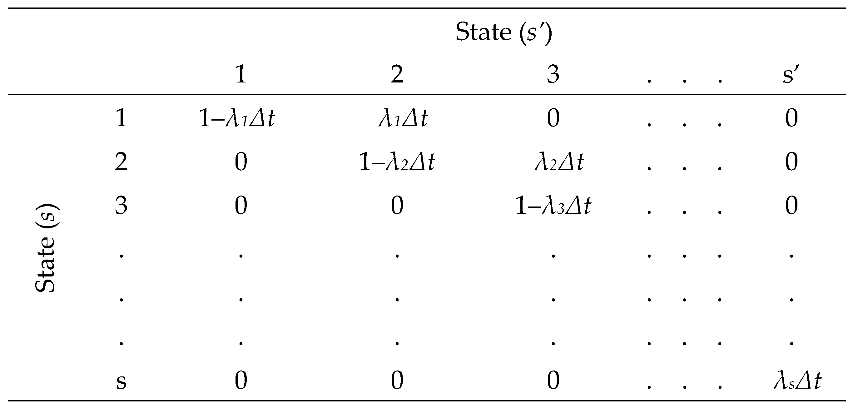
Then, the transition intensity (λ) was calculated by sequentially differentiating Kolmogorov’s forward equations for a pure birth process. The equation was solved for a very small time interval (∆t), where a maximum of one state transition can occur. For a pure birth process, the initial transition matrix is defined as the product of transition intensity and time interval (i.e., λ_s∆t), as shown in Figure 1. This is a square matrix (s (current state) by s′ (succeeding state) where s = s′). An n-step transition matrix (based on the initial transition) determines the transition probability for any inspection time interval t.

The determination of a small time interval (∆t) value could be subjective. However, a general guideline can be set to create a time interval for only a single state transition. A Poisson distribution defines the number of events (in this case, the transition to another state) for a Markov process (pure birth process). The value of ∆t was set to make the probability of having more than one event a sufficiently small value.

The Markov method can be modified to meet some specific process requirements. For example, Caleyo et al. [20] have presented a method for incorporating additional growth-rate factors, such as soil conditions or the surrounding environment for external corrosion (based on empirical data), in the transition probability to describe the degradation level better. As Bushinskaya [21] demonstrated, the Markov method based on the pure birth process can be transposed to create a pure death process and compute the strength of the pipeline instead of the degradation. Li et al. [22] proposed an empirical method for formulating the transition probability. This method defined the corrosion states (i.e., deterioration ranges for each state) first, then the transition probability matrix was calculated by categorizing the expected deterioration per year (for the time horizon under consideration) under each state and analyzing these yearly deteriorations under each state independently.

3.4. Observation

Because of the limitations of ILI equipment and methods, the actual state of the pipeline can be hard to accurately observe. The POMDP observation values are what is reported as a reading from the ILI. The observation, however, can be related to the actual states through a probability distribution. This can be determined empirically or by a numerical analysis of the main contributors to these discrepancies.

Dann and Maes [23] illustrated four sources of ILI tool errors: detection errors, sizing errors, false call errors, and reporting threshold errors. Detection errors occur when the ILI equipment fails to detect existing corrosion. This error increases as the size of the corrosion decrease since small-size corrosion defects are easy to miss. The probability of detection (PoD) is defined as a function of defect depth (d > 0) and tool detection capacity (k_d) [16]. The tool detection capacity can be replaced by mean detection thresholds (defined as 1/k_d), which are information supplied by the manufacturers.

$$PoD=1-e^{-d{k}_d}$$

(6)

where

$$d = \mathrm{defect}\mathrm{depth};k_d = \mathrm{tool} \mathrm{detection} \mathrm{capacity}$$

Random measurement errors (ϵ) are generated due to the inherent nature of the tool. Thus, they cannot be avoided. This error can be formulated as an independent, normally distributed function [16]. The actual corrosion defect depth d is the sum of the depth reading of the equipment (d_r) and the measuring error (ϵ).

False calls are created when ILI equipment reports a defect that does not exist in the pipeline. According to Dann and Maes [23], the cause for this error can be attributed to noises in the reading process or the misinterpretation of readings. This error depends on the ILI tool’s state (quality) and the corrosion defect’s size. In this case, the probability of committing an error increases as the size of the defect increases. Therefore, the probability of making a true call (PoTC) in the ILI reading is defined as a function of the equipment working condition factor (k_w) and the depth of the defect (d).

$$PoTC=1-e^{-d{k}_w}$$

(7)

where

$$d = \mathrm{defect}\mathrm{depth};k_w = \mathrm{tool} \mathrm{detection} \mathrm{capacity}$$

Reporting threshold errors arise from the limitations of the ILI equipment. Most manufacturers label their equipment’s threshold level, meaning any corrosion defects below this level will not be detected. All sources of error identified above refer to defects above this threshold level.

3.5. Reward

The cost of maintenance operations comprises the reward function in this model. Heidarydashtarjandi, Prasad-Rao, and Groth [6] proposed the sum of inspection, maintenance action cost (defined as a function of state and action), and failure cost as the reward function. The failure cost was computed by defining the types of failures (such as small leaks, large leaks, and ruptures) and their probability under each state. This cost integrated the risk associated with failures due to unexecuted maintenance actions. Zhang and Zhou (2014) detailed the maintenance cost, which incorporates excavation, sleeving, and recoating, which are commonly applied to repair pipelines. All the cost computation approaches discussed in the articles can be adopted for POMDP reward function computation. However, the inspection cost would have a meaningful impact if the POMDP model is formulated in such a way that different inspection intervals are considered in the problem.

$$R_{S,A}=C{M}_{S,A}+C{F}_S \left(+CI\right)$$

(8)

where

$${CM}_{S,A}—\mathrm{the} \mathrm{cost} \mathrm{of} \mathrm{maintenance} (\mathrm{costs} \mathrm{such} \mathrm{as} \mathrm{excavation}, \mathrm{sleeving}, \mathrm{coating}, \mathrm{labor}, \mathrm{and} \mathrm{equipment})$$

$${CF}_S—\mathrm{the} \mathrm{cost} \mathrm{of} \mathrm{failure}$$

$$CI—\mathrm{the} \mathrm{cost} \mathrm{of} \mathrm{inspection}$$

4. Numerical Examples

Two numerical examples were formulated to demonstrate the implementation of the proposed model in the preceding section. The first example implements a maintenance optimization method for a single pipeline. Based on this, this section discussed a two-pipeline system maintenance optimization method as another significantly more complex example.

4.1. Numerical Example 1

4.1.1. Model Formulation

Numerical values from various articles have been compiled in order to create a POMDP model to demonstrate the implementation of the proposed approach. The MDP model proposed by Heidarydashtarjandi, Prasad-Rao, and Groth [6] defined eight equally spaced deterioration states with four actions (do-nothing, inhibitor application, pigging, and replacement) to mitigate deterioration. The transition matrix (do-nothing action) was adopted by modifying data from the article. Thus, the probability of a pipeline inspected to be in each state is computed using a Monte Carlo simulation. A pure birth transition intensity was computed using this probability. Then, the intensity was used to find the probability of transitioning to the succeeding state and remaining in the current state (for ∆t = 0.0005 years). For the inspection interval of 5 years, a 10,000-step transition matrix was used to define the transition probability.

Table 1. State probability and transition intensity (modified from the source: Heidarydashtarjandi, Prasad-Rao, and Groth [6])).

State	Probability of the State	Transition Intensity (λi) in Years
1	0.01%	1.842068074
2	1.96%	0.043999123
3	58.87%	0.221188399
4	32.39%	0.173228351
5	3.62%	0.011165733
6	1.10%	0.00227737
7	0.55%	0.001113594
8	1.49%	0

and

Table 2. Transition matrix using a pure birth Markov process and n-step transition do-nothing (modified from the source: Heidarydashtarjandi, Prasad-Rao, and Groth [6]).

		State (S′)
		1	2	3	4	5	6	7	8
State (S)	1	0.000	0.822	0.111	0.051	0.016	0.000	0.000	0.000
	2	0.000	0.803	0.117	0.060	0.020	0.000	0.000	0.000
	3	0.000	0.000	0.331	0.414	0.250	0.005	0.000	0.000
	4	0.000	0.000	0.000	0.421	0.561	0.018	0.000	0.000
	5	0.000	0.000	0.000	0.000	0.946	0.054	0.000	0.000
	6	0.000	0.000	0.000	0.000	0.000	0.989	0.011	0.000
	7	0.000	0.000	0.000	0.000	0.000	0.000	0.994	0.006
	8	0.000	0.000	0.000	0.000	0.000	0.000	0.000	1.000

present these parameters for the model.

For the observation matrix, the ILI errors were estimated based on the numerical example published by Dann and Maes (2018). Mean values of 0.93 and 0.9 were obtained for the PoD and PoTC (actual depth 40–80% of wall thickness and mean detection 10–25% of wall thickness). Based on this, a reading error of 15% was considered for the numerical analysis. In other words, a 1.2 state deviation was estimated as the error in reading for an eight-state model (i.e., 1.2 = 8 ∗ 0.15). The other factor considered in the model was how the observation errors were applied. The first case defined the multiple observed states overlapping with actual states, whereas the second categorized the observed states as only pre-defined multiple actual states (see

Table 3. Observation probability matrix.

		Observation (O)
		1	2	3	4	5	6	7	8
State (S)	1	1.00	0.00	0.00	0.00	0.00	0.00	0.00	0.00
	2	0.00	0.80	0.20	0.00	0.00	0.00	0.00	0.00
	3	0.00	0.20	0.60	0.30	0.00	0.00	0.00	0.00
	4	0.00	0.00	0.20	0.40	0.32	0.25	0.00	0.00
	5	0.00	0.00	0.00	0.30	0.35	0.25	0.00	0.00
	6	0.00	0.00	0.00	0.00	0.33	0.25	0.30	0.00
	7	0.00	0.00	0.00	0.00	0.00	0.25	0.50	0.00
	8	0.00	0.00	0.00	0.00	0.00	0.00	0.20	1.00
(a) Overlapping observed states
State (S)	1	1.00	0.00	0.00	0.00	0.00	0.00	0.00	0.00
	2	0.00	1.00	0.00	0.00	0.00	0.00	0.00	0.00
	3	0.00	0.00	0.50	0.50	0.00	0.00	0.00	0.00
	4	0.00	0.00	0.50	0.50	0.00	0.00	0.00	0.00
	5	0.00	0.00	0.00	0.00	0.30	0.30	0.30	0.00
	6	0.00	0.00	0.00	0.00	0.35	0.35	0.35	0.00
	7	0.00	0.00	0.00	0.00	0.35	0.35	0.35	0.00
	8	0.00	0.00	0.00	0.00	0.00	0.00	0.00	1.00
(b) Non-overlapping observed states

).

Finally, the reward function combined the maintenance and failure cost for each state–action pairing. The failure costs were adopted from Heidarydashtarjandi, Prasad-Rao, and Groth [6], whereas the failure-type probability was generated based on some understanding of the nature of the failures across the states (

Table 4. Cost of failure (modified from the source: Heidarydashtarjandi, Prasad-Rao, and Groth [6].)

	Cost of Failure	Probability of Failure
		1	2	3	4	5	6	7	8
No failure	0.00	0.90	0.69	0.45	0.30	0.05	0.00	0.00	0.00
Small leak	1000.00	0.10	0.30	0.50	0.60	0.70	0.60	0.20	0.00
Large leak	8000.00	0.00	0.01	0.05	0.10	0.20	0.30	0.60	0.80
Rapture	40,000.00	0.00	0.00	0.00	0.00	0.05	0.10	0.20	0.20

). The reward for do-nothing decreases as the deterioration of the pipeline increases due to the loss of potential savings by prolonged life through maintenance. Inhibitors, pigging, and replacement can only be applied to certain states, and the remaining states were assigned large values.

Table 5. Reward function (values).

		States
		1	2	3	4	5	6	7	8
Action	Do nothing	−20	−200	−300	−400	−500	−600	−700	−800
	Inhibitors	−180	100	250	300	−5500	−5500	−5500	−5500
	Pigging	−5500	−5500	−5500	−400	1100	1700	2000	−5500
	Replace	−5500	−5500	−5500	−5500	−5500	−5500	200	1580

presents the reward values applied to the test model.

4.1.2. Results

MATLAB MDPToolBox [24] was used to solve this problem. Even though the tool primarily solves the MDP model, it has integrated packages (pomdp and pomdpsolve) to convert POMDP models into MDP forms using belief states. The test model was formulated for a 5-year operational run of a pipeline. The backward iteration of the Bellman equation method solver was used to solve the problem. Only ten belief states were defined for each deterioration state in order to meet the computation limit of MATLAB. An MSI GT72S 6QE Dominator laptop with Intel Core i7-6820 and 48 GB RAM was used to run the model.

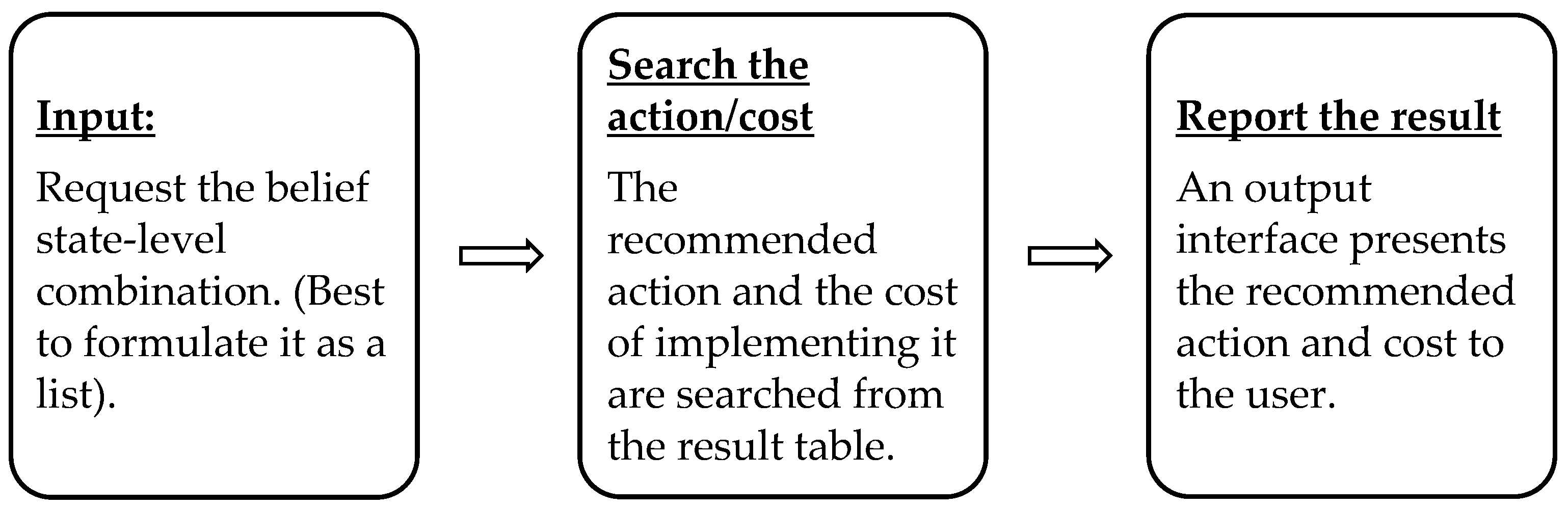
For both observation matrix formulations, the solver reported a do-nothing action for state 1, the application of inhibitors for states 2 and 3, pigging for states 3 through 6, and replacement for states 7 and 8 when the POMDP model considered all states that can be fully observed. In other words, this result is what would be attained when the model is formulated as an MDP (i.e., the states are fully observable). The main objective of this modeling was to obtain a recommendation for optimal maintenance operations for different belief states of pipeline deterioration. Accordingly, the result of the model consisted of recommendations for 19,448 belief states combinations. These are obtained from the ten belief states (for each of the eight states) that add up to 1. The optimal action and its cost were given for these belief states. A user interface will be required to read the maintenance action for the specific belief states′ combination since the reported combination of belief states is large. Figure 2 gives the general framework of this interface. Do-nothing was recommended at 80.5% (15,662 combinations) and 72% (13,996 combinations) for overlapping and no-overlapping models, respectively. Inhibitors, pigging, and replacement were reported at 1.2% and 1.4%, 3.3% and 3.8%, and 15% and 22.9%, respectively, for the two models.

4.2. Numerical Example 2

4.2.1. Model Formulation

Pipeline maintenance can be performed based on routing and segments, where each consists of multiple pipes. If maintenance decisions need to be made on the routing/segment level, a systemic approach would have to be applied to consider the interaction of components. The individual pipeline model components described above were combined to construct a two-pipeline system model. For identical pipes and ILI readings, the states of the system were formulated as s₁, s₂ (Ɐs₁ ∈ S₁, Ɐs₂ ∈ S₂), which combined the states of each pipe [25]. It is assumed that the deterioration of each pipeline is independent and identical. Dependent pipelines and multi-component pipeline systems′ [26] deterioration were considered outside of the scope of this study. A total of 64 states were created for an eight-state pipeline system. The actions were considered to be the same since the pipeline system consists of identical pipes. The transition matrix was computed for the individual pipes, which were used to formulate the system’s transitions. Therefore, for a one state transition of this two-pipeline system, the transition matrix consisted of both pipes remaining in their current states, one of the pipes moving to the next state, and both pipes transitioning to the next state. A similar procedure was adopted to transform the matrix into an n-state transition matrix (

Table 6. Transition probability for a two-pipe system based on pipeline 1 (P1) and pipeline 2 (P2).

				State (S’)
			P1	1	1	1	1	1	1	1	1	2	2	2	2	2	2	.	.	.	8	8	8	8
			P2	1	2	3	4	5	6	7	8	1	2	3	4	5	6	.	.	.	5	6	7	8
	P1	P2		1	2	3	4	5	6	7	8	9	10	11	12	13	14	.	.	.	61	62	63	64
State (S)	1	1	1	0	0	0	0	0	0	0	0	0	0.68	0.09	0.04	0.01	0	.	.	.	0	0	0	0
	1	2	2	0	0	0	0	0	0	0	0	0	0.66	0.10	0.05	0.02	0	.	.	.	0	0	0	0
	1	3	3	0	0	0	0	0	0	0	0	0	0	0.27	0.34	0.21	0.01	.	.	.	0	0	0	0
	1	4	4	0	0	0	0	0	0	0	0	0	0	0	0.35	0.46	0.02	.	.	.	0	0	0	0
	1	5	5	0	0	0	0	0	0	0	0	0	0	0	0	0.78	0.04	.	.	.	0	0	0	0
	1	6	6	0	0	0	0	0	0	0	0	0	0	0	0	0	0.81	.	.	.	0	0	0	0
	1	7	7	0	0	0	0	0	0	0	0	0	0	0	0	0	0	.	.	.	0	0	0	0
	1	8	8	0	0	0	0	0	0	0	0	0	0	0	0	0	0	.	.	.	0	0	0	0
	2	1	9	0	0	0	0	0	0	0	0	0	0.66	0.09	0.04	0.01	0	.	.	.	0	0	0	0
	2	2	10	0	0	0	0	0	0	0	0	0	0.64	0.09	0.05	0.02	0	.	.	.	0	0	0	0
	2	3	11	0	0	0	0	0	0	0	0	0	0	0.27	0.33	0.20	0	.	.	.	0	0	0	0
	2	4	12	0	0	0	0	0	0	0	0	0	0	0	0.34	0.45	0.01	.	.	.	0	0	0	0
	2	5	13	0	0	0	0	0	0	0	0	0	0	0	0	0.76	0.04	.	.	.	0	0	0	0
	2	6	14	0	0	0	0	0	0	0	0	0	0	0	0	0	0.79	.	.	.	0	0	0	0
	.	.	.	.	.	.	.	.	.	.	.	.	.	.	.	.	.	.	.	.	.	.	.	.
	.	.	.	.	.	.	.	.	.	.	.	.	.	.	.	.	.	.	.	.	.	.	.	.
	.	.	.	.	.	.	.	.	.	.	.	.	.	.	.	.	.	.	.	.	.	.	.	.
	8	5	61	0	0	0	0	0	0	0	0	0	0	0	0	0	0	.	.	.	0.95	0.05	0	0
	8	6	62	0	0	0	0	0	0	0	0	0	0	0	0	0	0	.	.	.	0	0.99	0.01	0
	8	7	63	0	0	0	0	0	0	0	0	0	0	0	0	0	0	.	.	.	0	0	0.99	0.01
	8	8	64	0	0	0	0	0	0	0	0	0	0	0	0	0	0	.	.	.	0	0	0	1.00

).

The observations and reward functions have been calculated by multiplying the respective state’s values.

Table 7. Observation probability (overlapping case) and reward for a two-pipe system based on pipeline 1 (P1) and pipeline 2 (P2).

				State (S’)
			P1	1	1	1	1	.	.	.	8	8	8	8
			P2	1	2	3	4	.	.	.	5	6	7	8
	P1	P2		1	2	3	4	.	.	.	61	62	63	64
State (S)	1	1	1	1.00	0	0	0	.	.	.	0	0	0	0
	1	2	2	0	0.90	0.20	0.00	.	.	.	0	0	0	0
	1	3	3	0	0.10	0.60	0.30	.	.	.	0	0	0	0
	1	4	4	0	0	0.20	0.40	.	.	.	0	0	0	0
	.	.	.	.	.	.	.	.	.	.	.	.	.	.
	.	.	.	.	.	.	.	.	.	.	.	.	.	.
	.	.	.	.	.	.	.	.	.	.	.	.	.	.
	8	5	61	0	0	0	0	.	.	.	0.35	0.25	0	0
	8	6	62	0	0	0	0	.	.	.	0.33	0.25	0.30	0
	8	7	63	0	0	0	0	.	.	.	0	0.25	0.50	0
	8	8	64	0	0	0	0	.	.	.	0	0	0.20	1.00
				Reward
	P1			1	1	1	1	.	.	.	8	8	8	8
	P2			1	2	3	4	.	.	.	5	6	7	8
				1	2	3	4	.	.	.	61	62	63	64
Action (A)	1			−40	−220	−320	−420	.	.	.	−1300	−1400	−1500	−1600
	2			−360	−80	70	120	.	.	.	−11,000	−11,000	−11,000	−11,000
	3			−11,000	−11,000	−11,000	−5900	.	.	.	−4400	−3800	−3500	−11,000
	4			−11,000	−11,000	−11,000	−11,000	.	.	.	−3920	−3920	1780	3160

gives the observation probabilities for the overlapping case of the model’s formulation and the cost of taking a given action under a specific state.

4.2.2. Result

The same solver tool, i.e., MDPToolBox [24], was used on the same laptop to run the two-pipeline system POMDP model. Three belief states were defined for each deterioration state in order to meet the computation limit of MATLAB (lack of available memory size). The backward iteration of the Bellman equation method was also selected from the solver toolbox.

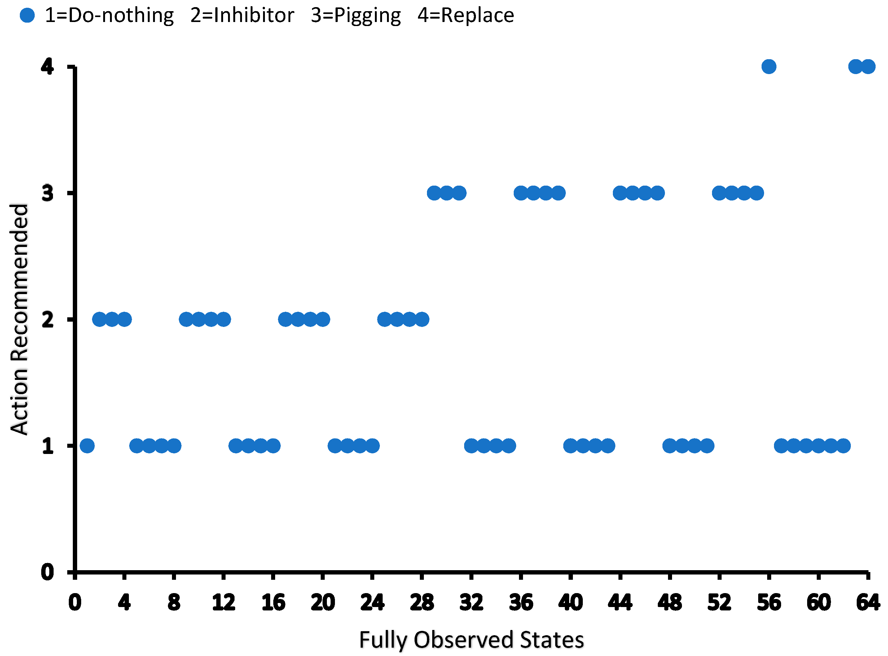
The two-pipeline system also reported the same maintenance action for the fully observable state under the two setups. The recommended actions for each observable deterioration state are given in Figure 3.

The result of this model run comprised 45,760 combinations of belief states for the 64 states of pipeline deterioration. The distribution of the recommended actions is given in

Table 8. Recommended action percentage for single and two-pipeline systems.

		Single Pipeline	Two Pipelines System
Action	Do-nothing	64.2%	87.0%
	Inhibit	15.0%	1.8%
	Pigging	18.3%	10.7%
	Replace	2.5%	0.5%

, along with a three-belief-state-run of the single pipeline model for comparison.

The run time is significantly increased for the two-pipeline system, as expected. For the single pipeline, it took 8 milliseconds (fully observable states) and 3 milliseconds (POMDP) for the first observation setup, whereas the second setup needed 0.7 milliseconds (fully observable states) and 0.6 milliseconds (POMDP) to obtain the results. The two-pipeline system required 2 milliseconds (fully observable states) and 1100 milliseconds (POMDP) for the first setup, while 1 millisecond and 300 milliseconds run times were obtained for the second setup.

4.3. Discussion

Analysis of the recommended action under each observation model can aid the development of a framework that defines the belief state combination for taking each action. After screening out the belief states for each action, the level and combination of these states can be studied to determine the deterioration state level. With such a kind of demarcation, the decision alternative on the type of maintenance action can better be estimated under different uncertainty levels of deterioration.

The transitional probability was computed for time (∆t) and inspection interval time (T) values equal to 0.0005 years and 5 years, respectively. However, these values are not necessarily fixed and should be adjusted to meet the needs of specific pipelines. The transitional probability change significantly impacts each belief state’s recommended actions. It determines which actions are allowed to be taken in a particular state. The probability matrix for specific maintenance actions can be computed using historical data, expert-opinion analysis methods, or a combination of both. For the POMDP model considered in this paper, only inline instrumentational errors have been considered as the sources of the observational disparity. Nevertheless, other sources of errors can be integrated, including the maintenance technician’s skill level, pipeline locations, surroundings, and the type of product transported. The variation in the formulation of the observation for one- and two-pipe systems has a limited impact on the overall recommended action except for the run time. When more ILIs are considered, this variation influences the actions. The cost of maintenance can be computed from the actual operating expenses and service charges. A more detailed assessment of these costs would have to be performed to estimate the true value. It is possible to exclude the cost of failure if the deterioration states considered in the model are located well above the risk limits. This means that pipelines will be replaced before reaching risky deterioration levels. Inspection costs can be added to the reward if they can be related to the action. Otherwise, it will not have any impact on the reward since it is a constant value.

5. Conclusions

The accurate determination of corrosion in pipelines is difficult in most real-world cases. These inaccuracies emanate from different sources, including equipment errors, human limitations, the environment, and/or the nature of pipeline transportation systems. Maintenance operations are performed with all these limitations, which can lead to additional resource expenditure and maintenance costs. This paper proposed a POMDP maintenance optimization model, which accommodates these inaccuracies (using equipment error as an example) to identify the pipelines′ operating condition and propose the optimal maintenance action. Each state represented a uniformly progressive level that covered the entire corrosion deterioration range. The different corrosion mitigation methods were considered as maintenance actions for the model. Transition intensity was used to define the probability of transition between states. The analysis of the inspection errors formulated the observation probability. The cost of maintenance and failure made up the reward function for a given state and action.

A single-pipeline and two-pipeline system corrosion maintenance optimization problem model were formulated to demonstrate the implementation of the proposed model. The result of the model run showed that the optimal action and the cost of implementing it could be obtained for the different probabilities of deterioration states. This loosens the need for a strictly defined deterioration state, which would provide flexibility in decision-making for maintenance technicians and managers.

The implementation of the POMDP for optimizing maintenance operations can be further extended in different directions. The problem formulation and size of the model could be enhanced to create a very complex pipeline system. With this approach, the study could address the implementation of the POMDP method for the maintenance of a system consisting of tens and hundreds of pipelines. The model could also include the interaction among different components of the pipeline system. Furthermore, the method can be explored for its suitability in determining maintenance criticality assessment and policy optimization. Maintenance operations criticality can improve the utilization of limited maintenance resources. Different preventive maintenance policies, including multi-policy approaches, could also be adopted in the implementation of maintenance actions in the models.

Companies in the oil and gas industries carry out pipeline maintenance under uncertain conditions. The proposed model attempts to address these uncertainties to improve the pipeline’s overall performance and safety. Maintenance is one of the industry’s major functions that affect the success of a company.