Crossover Rate Sorting in Adaptive Differential Evolution

Abstract

Differential evolution (DE) is a popular and efficient heuristic numerical optimization algorithm that has found many applications in various fields. One of the main disadvantages of DE is its sensitivity to parameter values. In this study, we investigate the effect of the previously proposed crossover rate sorting mechanism on modern versions of DE. The sorting of the crossover rates, generated by a parameter adaptation mechanism prior to applying them in the crossover operation, enables the algorithm to make smaller changes to better individuals, and larger changes to worse ones, resulting in better exploration and exploitation. The experiments in this study were performed on several modern algorithms, namely L-SHADE-RSP, NL-SHADE-RSP, NL-SHADE-LBC and L-NTADE and two benchmark suites of test problems, CEC 2017 and CEC 2022. It is shown that crossover rate sorting does not result in significant additional computational efforts, but may improve results in certain scenarios, especially for high-dimensional problems.

1. Introduction

The area of computational intelligence (CI) in recent years has undergone significant development by researchers from around the world. The reason for such interest is the ability of the approaches, such as neural networks (NNs), fuzzy logic (FL) and evolutionary computation (EC), to solve complex problems, which were considered unsolvable before. Among evolutionary computation algorithms, and numerical optimization methods in particular, differential evolution (DE) has become one of the most popular algorithms. The reason for such popularity is the simplicity of the basic algorithm and its high efficiency even for complex, multi-dimensional problems. Since the original algorithm proposal by Storn and Price [1], there have been many modifications proposed for DE, seeking to eliminate its weak sides, such as high sensitivity to parameter values.

Most of the studies on differential evolution are aimed at proposing new parameter adaptation techniques or new mutation and crossover strategies; however, some research considers different algorithmic schemes and population control strategies. The adaptive and self-adaptive mechanisms were proposed in SaDE [2], jDE [3], JADE [4], SHADE [5], MPEDE [6], jSO [7], and many others. Several surveys, such as [8,9], as well as more recent ones [10,11], indicate that most studies on DE are searching for a balance between exploration and exploitation properties, which is important for preventing premature convergence and improving the final solutions. One of such techniques is the crossover rate sorting (CRS), originally proposed in [12], where it was applied to the JADE algorithm.

In this study, the crossover rate sorting is applied to more modern DE versions, which were presented for the IEEE Congress on Evolutionary Computation (CEC) competitions on bound-constrained single-objective numerical optimization. The reason for this is to check the effect of this modification on more complex approaches than JADE, as it is well known that more complex and well-performing algorithms are more difficult to improve. For the purposes of this study, four baseline approaches have been chosen, in particular, L-SHADE-RSP [13], NL-SHADE-RSP [14], NL-SHADE-LBC [15] and the recently proposed L-NTADE [16]. Two benchmarks were chosen for testing, namely CEC 2017 [17] and CEC 2022 [18], due to their different number of functions, different set of dimensions and algorithms efficiency comparison methods. The main contributions of this study are the following:

• The crossover rate sorting is capable of significantly improving the performance of modern DE algorithms, although there are cases where it decreases the performance;
• The crossover rate sorting has larger effect on high-dimensional problems, as well as multimodal problems;
• For relatively simple unimodal problems, sorting the crossover rates significantly increases the convergence speed but at the cost of decreased diversity.
• The crossover rates saved in the memory cells are much larger if the crossover rate sorting is applied.

The rest of the paper is organized as follows. Section 2 contains an overview of related work, the third section describes the proposed approach, the fourth section contains the experimental setup and results, then a discussion of the results is provided, and the last section concludes the paper.

2. Materials and Methods

2.1. Differential Evolution

Like every evolutionary algorithm, the DE begins with initializing a population of solutions, randomly distributed in a search space. The initial population size is N, and the individuals are D-dimensional points, $x_i=(x_{i,1},x_{i,2},\cdots ,x_{i,D})$, $i=1,\cdots ,N$, generated as follows:

$$x_{i,j}=x_{lb,j}+rand\times (x_{ub,j}-x_{lb,j}).$$

(1)

where $j=1,\cdots ,D$, $x_{ub,j}$ and $x_{lb,j}$ are the upper and lower boundaries.

The main loop of DE consists of three operations: mutation, crossover and selection. The mutation operator is a main feature of DE, and it generates donor vector $v_{i,j}$ using individuals from the population and a scaling factor parameter F as follows:

$$v_{i,j}=x_{r1,j}+F\times (x_{r2,j}-x_{r3,j}),$$

(2)

where $x_{i,j}$ is the j-th coordinate of the i-th solution, and indexes i, $r1$, $r2$ and $r3$ are different from each other. The presented strategy is called rand/1, and was presented in [19] together with several other strategies, such as rand/2, best/1, best/2. The scaling factor parameter was originally proposed to be set in range $[0,2]$; however, most studies nowadays set it in the $[0,1]$ range. The differential evolution is highly sensitive to this setting, thus requiring adaptive schemes to be applied.

The crossover step combines the genetic information of mutant vector $v_i$ and the target vector $x_i$ to obtain an offspring, called trial vector $u_i$. There are two popular crossover schemes in DE, namely exponential and binomial, the latter being used more frequently. The binomial crossover uses a parameter value $Cr$ and works as follows:

$$u_{i,j}=\left\{\begin{array}{cc}{v}_{i,j},\hfill & \mathrm{if}rand(0,1)<Cr\mathrm{or}j=jrand\hfill \\ x_{i,j},\hfill & \mathrm{otherwise}\hfill \end{array}\right.$$

(3)

where $Cr$ is the crossover rate, and $jrand$ is a randomly generated index in $[1,D]$, required to make sure that at least one component is taken from the mutant vector. Without $jrand$, small $Cr$ values may result in evaluating the same vector, which would be a waste of computational resource. However, recent studies show that evaluating the same vector may still be an issue in DE [20].

Once the trial vector $u_i$ is generated, it is checked to be within the upper and lower boundaries $x_{ub,j}$ and $x_{lb,j}$, and if not, a bound-constraint handling method is applied, for example, midpoint target.

In DE, a greedy selection mechanism is applied, i.e., the trial vector $u_i$ replaces the target vector $x_i$ only if it has better fitness. This scheme can be described as follows:

$$x_i=\left\{\begin{array}{cc}{u}_i,\hfill & \mathrm{if}f\left(u_i\right)\le f\left(x_i\right)\hfill \\ x_i,\hfill & \mathrm{if}f\left(u_i\right)>f\left(x_i\right).\hfill \end{array}\right.$$

(4)

Despite the efficiency of such an approach, some attempts were made to modify the selection step, for example, with neighborhood information [21] or by introducing novel algorithmic schemes with two populations [16].

2.2. Parameter Adaptation for Mutation and Crossover

The simplicity and efficiency of DE made it a highly popular numerical optimization algorithm, leading to vast amounts of studies. As the current study is not focused on a comprehensive review, interested readers are redirected to several older surveys, such as [8,9,22], as well as more recent ones [10,11], and studies dedicated to parameter adaptation [23]. Moreover, several studies have made attempts to design parameter adaptation techniques automatically with genetic programming [24] or neuroevolution [25].

The most commonly used parameter adaptation mechanism, which tunes both scaling factor F and crossover rated $Cr$, was introduced in the SHADE algorithm [5] and further extended in L-SHADE [26] by adding population size control called LPSR. The parameter adaptation in SHADE originated from JADE and maintains a set of memory cells, containing averaged successful values of F and $Cr$. These memory cells are updated at the end of each generation based on which the values result in an improvement in terms of fitness. However, since the JADE algorithm, the most well-performing DE methods use almost the same adaptation scheme for the crossover rate, although its influence on the performance is crucial [27]. In SHADE, the crossover rates are generated with normal distribution and $0.1$ variance from the memory cell values $M_{Cr,r}$, where $r\in [1,H]$ is chosen randomly for each individual, and H is the memory size as follows:

$$Cr=randn(M_{Cr,r},0.1),$$

(5)

where $randn(m,\sigma )$ is a normally distributed random value. If $Cr$ generated for the i-th individual is outside $[0,1]$, it is truncated to this range. The update of the memory cell is performed with the weighted Lehmer mean:

$$mea{n}_{wL}=\frac{{\sum }_{j=1}^{|S^{Cr}|}{w}_j{\left(S_j^{Cr}\right)}^2}{{\sum }_{j=1}^{|S^{Cr}|}{w}_j{S}_j^{Cr}},$$

(6)

where $w_j={S_{\Delta f}^{Cr}}_j/\left({\sum }_{k=1}^{\left|S\right|}{S_{\Delta f}^{Cr}}_k\right)$, $S^{Cr}$ is a set of successful crossover rates. The values are updated as follows:

$$M_{Cr,k}^{g+1}=0.5(M_{Cr,k}^g+mea{n}_{(wL,Cr)}),$$

(7)

where g is the current generation number, and k is the index of the memory cell to be updated, iterated in the range $[1,H]$.

Various studies have investigated ways of improving DE crossover. For example, in [28], the repairing of the crossover rate was proposed, which considered the actual rate of the crossover applied to certain individuals instead of the set $Cr$ value. This enabled the more accurate tuning of $Cr$ and increased performance in certain scenarios. In [29], the hybrid linkage crossover (HLX) is proposed, aimed at detecting the linkages between pairs of variables and consisting of three parts: constructing linkage matrix, grouping variables, and applying group-wise crossover. In [30], the rotating crossover operator (RCO) is proposed to mitigate the problem of inefficient crossover due to rotated objective function landscape. The RCO enables us to adjust the rotation vectors, resulting in more efficient utilization of the computational resource. In [31], the superior–inferior (SI) crossover scheme is considered, which was developed to improve the diversity of the population when individuals are excessively clustered. If this is the case, the SI scheme recombines superior and inferior individuals in the crossover; otherwise, the superior–superior scheme is applied. Several studies, such as [32,33], applied several crossover strategies to generate offspring, combining exponential and binomial crossover.

In [12], the crossover rate sorting was proposed for the JADE algorithm, and the modification was called JADE_sort. The sorting was performed according to fitness values, with smaller $Cr$ values assigned to better target vectors. For the sorting to be possible, all $Cr$ values were generated before the crossover step. In addition to this, the scheme retention mechanism was proposed to improve local search. The JADE_sort was shown to improve performance in many cases, although it failed to do so on hybrid composition functions. The same sorting scheme was applied in LADEwSE in [34], as well as NL-SHADE-RSP [14] and NL-SHADE-LBC [15], but its effects were not studied. In the next subsection, the application of crossover rate sorting will be considered.

2.3. Proposed Approach

The idea of sorting a pool of generated crossover rates before applying them in creating offspring is relatively straightforward, and can be applied to most JADE and SHADE-based algorithms. Nevertheless, it is not widely applied in most well-performing DE algorithms, judging by the top algorithms in the CEC 2021 and CEC 2022 competitions. Here, in addition to the NL-SHADE-RSP and NL-SHADE-LBC algorithms, L-SHADE-RSP and L-NTADE will be considered, for which the crossover rate sorting was not applied before. For L-SHADE-RSP [13], the modification is quite simple; however, the L-NTADE algorithm [16], which has a different algorithmic structure, requires a more thorough discussion.

L-NTADE maintains two populations instead of one on the classical DE scheme. The first population is the continuously updated population of newest solutions $x^{new}$, while the second one contains the best individuals from the whole search, and is called the top population $x^{top}$. The idea of dividing the population in two parts was inspired by the unbounded differential evolution approach, proposed in [35]. The parameter adaptation applied in L-NTADE is the same success-history adaptation, as in L-SHADE; and thus, a pool of crossover rates $C{r}_i$, $i=1\cdots N$ can be generated at the beginning of the generation, before creating new solutions with mutation and crossover. However, in L-NTADE, there are several different mutation strategies applied, which combine individuals from both populations in a way similar to the current-to-pbest strategy. If the target vector is chosen from the newest population, the index $r1$ of the target vector to be used is generated randomly. In this study, the r-new-to-ptop/n/t is used, described as follows: $v_{i,j}=x_{r1,j}^{new}+F\times (x_{pbest,j}^{top}-x_{i,j}^{new})+F\times (x_{r2,j}^{new}-x_{r3,j}^{top})$.

Random sampling of the $r1$ index from the newest population means that if there are N crossover rates, $C{r}_i$ generated and sorted before the crossover, then some of them can be used twice within the same generation. However, this should not be a major problem, as the $Cr$ values are used for the random choice of donor vector components to be taken into the offspring solution. The selection step in L-NTADE updates an individual in the newest population with index $nc$, iterated from 1 to current population size N, but the trial vector’s fitness is compared to the fitness of the $r1$-th individual:

$$x_{nc}=\left\{\begin{array}{cc}{u}_i,\hfill & \mathrm{if}f\left(u_i\right)\le f\left(x_{r1}^n\right)\hfill \\ x_{nc},\hfill & \mathrm{if}f\left(u_i\right)>f\left(x_{r1}^n\right).\hfill \end{array}\right.$$

(8)

This means that it is possible in L-NTADE_s, with the crossover rate sorting, to generate two new successful solutions with the same $Cr$ value; hence, the same value is used in updating memory cells in the success-history adaptation mechanism.

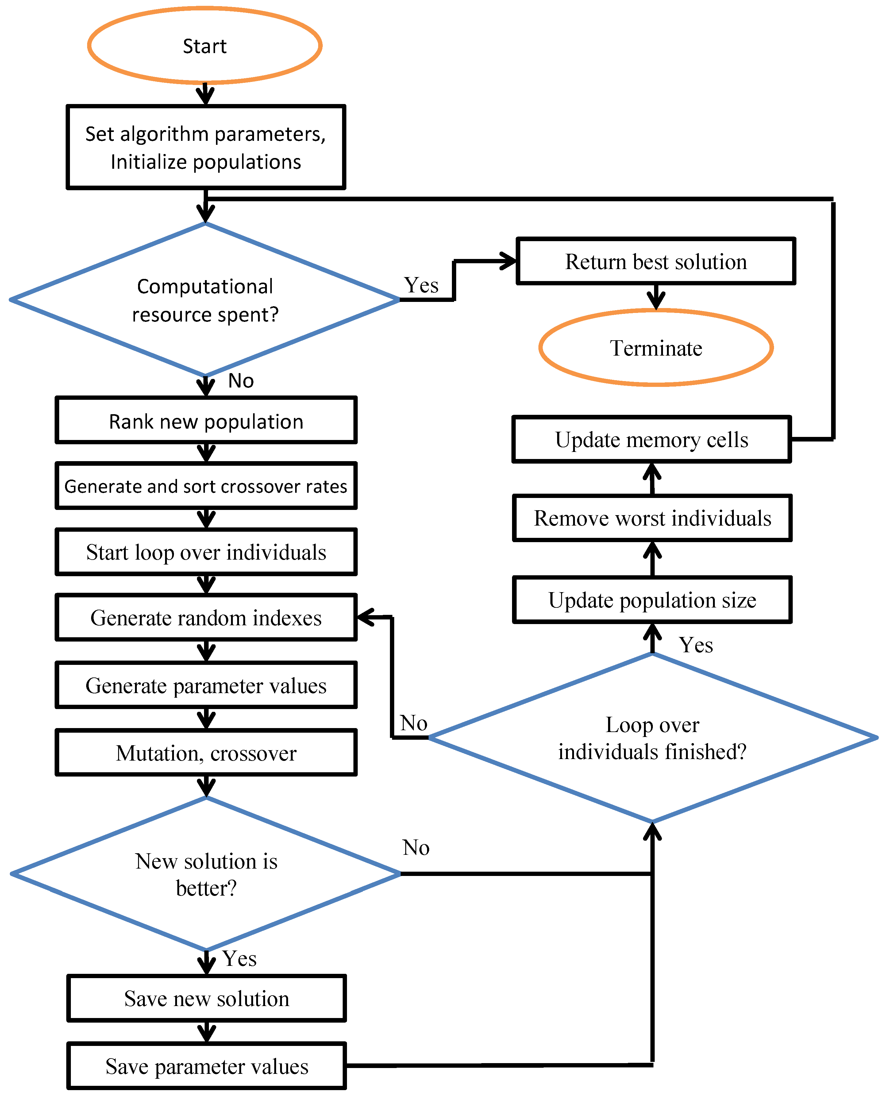
The pseudocode of the L-NTADE_s is shown in Algorithm 1.

Algorithm 1 L-NTADE_s

1: Input: D, $NF{E}_{max}$, $N_{max}$, objective function $f\left(x\right)$ 2: Output: $x_{best}^{top}$, $f\left(x_{best}^{top}\right)$ 3: Set $N_{cur}^0=N_{max}$, $N_{min}=4$, $H=5$, $M_{F,r}=0.3$, $M_{Cr,r}=1$ 4: Set $pb=0.3$, $k=1$, $g=0$, $nc=1$, $kp=0$, $pm=2$ 5: Initialize population $(x_{1,j}^{new},...,x_{N_{max},j}^{new})$ randomly, calculate $f\left(x^{new}\right)$ 6: Copy $x^{new}$ to $x^{top}$, $f\left(x^{new}\right)$ to $f\left(x^{top}\right)$ 7: while$NFE<NF{E}_{max}$do 8:     $S_F=\varnothing$, $S_{Cr}=\varnothing$, $S_{\Delta f}=\varnothing$ 9:     Rank either $x^{new}$ by $f\left(x^{new}\right)$ 10:     for $i=1$ to $N_{cur}^g$ do 11:         Current memory index $r=randInt[1,H+1]$ 12:         Crossover rates $C{r}_i=randn(M_{Cr,r},0.1)$ 13:         $C{r}_i=min(1,max(0,Cr))$ 14:     end for 15:     Sort crossover rates according to $f\left(x^{new}\right)$ 16:     for $i=1$ to $N_{cur}^g$ do 17:         $r1=randInt\left(N_{cur}^g\right)$ 18:         Current memory index $r=randInt[1,H+1]$ 19:         repeat 20:            $F_i=randc(M_{F,r},0.1)$ 21:         until $F_i\ge 0$ 22:         $F_i=min(1,F_i)$ 23:         repeat 24:            $pbest=randInt(1,N_{cur}^g\ast pb)$ 25:            $r2=randInt(1,N_{cur}^g)$ or with rank-based selection 26:            $r3=randInt(1,N_{cur}^g)$ 27:         until indexes $r1$, $r2$, $r3$ and $pbest$ are different 28:         Apply mutation to produce $v_i$ with $F_i$ 29:         Apply binomial crossover to produce $u_i$ with $C{r}_i$ 30:         Apply bound constraint handling method 31:         Calculate $f\left(u_i\right)$ 32:         if $f\left(u_i\right)<f\left(x_{r1}^{new}\right)$ then 33:            $u_i\to x^{temp}$ 34:            $F\to S_F$, $Cr\to S_{Cr}$ 35:            $\Delta f=f\left(x_{r1}^{new}\right)-f\left(u_i\right)$ 36:            $\Delta f\to S_{\Delta f}$ 37:            $x_{nc}^{new}=u_i$ 38:            $nc=mod(nc+1,N_{cur}^g)$ 39:         end if 40:     end for 41:     Get $N_{cur}^{g+1}$ with LPSR 42:     Join together $x^{top}$ and $x^{temp}$, sort and copy best $N_{cur}^{g+1}$ to $x^{top}$ 43:     if $N_{cur}^g>N_{cur}^{g+1}$ then 44:         Remove worst individuals from $x^{new}$ 45:     end if 46:     Update $M_{F,k}$, $M_{Cr,k}$ 47:     $k=mod(k+1,H)$ 48:     $g=g+1$ 49: end while 50: Return $x_{best}^{top}$, $f\left(x_{best}^{top}\right)$

The block-scheme of the algorithm is shown in Figure 1.

3. Results

3.1. Benchmark Functions and Parameters

The idea of this study is to evaluate the performance benefits delivered by the crossover rate sorting in different scenarios. For this purpose, two sets of test functions were chosen, namely CEC 2017 [17] and CEC 2022 [18]. The first benchmark, introduced for the Congress on Evolutionary Computation competition on single-objective numerical optimization in 2017 and used also in 2018, contains 30 test functions, including unimodal, multimodal, hybrid and composition functions and problem dimensions 10, 30, 50 and 100. The CEC 2022 contains 12 functions and dimensions 10 and 20, but sets a larger computational resource: $\mathrm{10,000}\ast D$ for CEC 2017 and $2\times {10}^5$ for $10\ast D$, ${10}^6$ for $20\ast D$ for CEC 2022. For CEC 2017, there are 51 independent runs and 30 runs for CEC 2022. In CEC 2022, the algorithms are compared not only by the best found objective function values but also by the convergence speed, unlike CEC 2017. This makes these two benchmarks different from each other, allowing the comprehensive testing of crossover rate sorting.

All developed algorithms were implemented in C++, compiled with GCC and ran under Ubuntu 20.04. Due to the large amount of computations required for the experiments, the algorithms were paralleled with OpenMPI 4.0.3, and ran on a cluster of 8 MD Ryzen 3700 PRO. The results’ post-processing was performed with Python 3.6.

3.2. Numerical Results

The parameter settings for the mentioned algorithms were taken from the original papers. For example, for L-SHADE-RSP, the initial population size was set to $N_{max}=75\ast D^{\frac{2}{3}}$ and memory size $H=5$; for NL-SHADE-RSP, the initial population size $N_{max}=30\ast D$, and memory size $H=20\ast D$; and for NL-SHADE-LBC, the population size $N_{max}=23\ast D$, and $H=20\ast D$. For the L-NTADE algorithm, the following values were used: $N_{max}=20\ast D$, selective pressure parameter $kp=3$, biased parameter adaptation coefficient $pm=4$, and mutation strategy r-new-to-ptop/n/t. These values were set, as they enable us to achieve good results on both CEC 2017 and CEC 2022 benchmarks. The algorithms with crossover rate sorting were marked with _s, e.g., L-SHADE-RSP_s. It should be mentioned that the NL-SHADE-RSP and NL-SHADE-LBC had the sorting procedure in their standard setting, so here, the standard setting is denoted as NL-SHADE-RSP_s and NL-SHADE-LBC_s.

The efficiency comparison of the tested algorithms was performed with the Mann–Whitney statistical test with normal approximation and tie-breaking to compare variants with and without crossover rates sorting. Using normal approximation is possible due to the sufficient sample sizes (30 or 51 independent runs). It also enables us to calculate the standard score (Z-score), which simplifies the reasoning and estimating the difference between algorithm variants. If the decision about the significance of such a difference is to be made, the significance level equal to $0.01$ is used, which corresponds to the threshold Z score of $\left|2.58\right|$ (two-tailed test). In addition to the Mann–Whitney test, the Friedman ranking procedure was used to analyze the performance of the algorithms. The ranks were calculated for every function and then summed, with lower ranks being better.

In the first set of experiments, the algorithms are compared on the CEC 2017 benchmark. The results are shown in

Table 1. Algorithms with and without crossover rate sorting, CEC 2017, Mann–Whitney tests and total standard score.

Algorithms	$10\ast \mathit{D}$	$30\ast \mathit{D}$	$50\ast \mathit{D}$	$100\ast \mathit{D}$
L-SHADE-RSP vs.	1/27/2	6/24/0	4/25/1	7/22/1
L-SHADE-RSP_s	(2.07)	(29.45)	(28.24)	(21.21)
NL-SHADE-RSP vs.	3/27/0	1/28/1	1/29/0	0/28/2
NL-SHADE-RSP_s	(12.67)	(3.23)	(8.59)	(−8.92)
NL-SHADE-LBC vs.	1/27/2	3/26/1	13/15/2	11/17/2
NL-SHADE-LBC_s	(−9.51)	(26.43)	(51.53)	(50.23)
L-NTADE vs.	0/28/2	1/22/7	2/19/9	4/15/11
L-NTADE_s	(−10.58)	(−27.31)	(−14.32)	(−32.69)

and

Table 2. Algorithms with and without crossover rate sorting, CEC 2017, and Friedman ranks.

Algorithm	$10\ast \mathit{D}$	$30\ast \mathit{D}$	$50\ast \mathit{D}$	$100\ast \mathit{D}$	Total
LSHADE-RSP	109.00	99.45	96.85	96.72	402.02
LSHADE-RSP_s	99.21	92.85	95.21	92.23	379.49
NL-SHADE-RSP	127.16	120.21	114.37	110.51	472.25
NL-SHADE-RSP_s	121.92	119.51	114.37	110.51	466.31
NL-SHADE-LBC	88.43	104.06	110.52	108.70	411.71
NL-SHADE-LBC_s	83.47	101.79	109.83	108.28	403.38
L-NTADE	109.83	104.54	98.81	106.25	419.43
L-NTADE_s	100.98	97.59	100.03	106.81	405.41

, the latter of which contains the Friedman ranking of the results.

The values in Table 1 shown in every cell are the number of wins/ties/losses of the algorithm without crossover rate sorting, and with it, the sum of these three equals the number of test functions. The number in brackets is the total standard score, i.e., sum of all standard scores of the Mann–Whitney test over all test functions. The results indicate that the effect of the sorting crossover rates is not always positive. For example, for L-NTADE, the sorting results in worse performance in most cases, although for $100\ast D$ functions, there are 4 improvements out of 30. However, the NL-SHADE-LBC algorithm receives significant improvements, as well as L-SHADE-RSP, which becomes better for 7 functions out of 30. At the same time, the NL-SHADE-RSP algorithm does not seem to be influenced by this modification, and its performance stays almost at the same level. The Friedman ranking demonstrates that the algorithms with crossover rate sorting received lower or equal ranks in almost all cases, except L-NTADE in $50\ast D$ and $100\ast D$.

Table 3. Algorithms with and without crossover rate sorting, CEC 2022, Mann–Whitney tests and total standard score.

Algorithms	$10\ast \mathit{D}$	$20\ast \mathit{D}$
L-SHADE-RSP vs.	4/8/0	4/8/0
L-SHADE-RSP_s	(27.44)	(25.92)
NL-SHADE-RSP vs.	6/5/1	2/9/1
NL-SHADE-RSP_s	(26.49)	(11.32)
NL-SHADE-LBC vs.	6/6/0	5/7/0
NL-SHADE-LBC_s	(36.62)	(31.43)
L-NTADE vs.	5/7/0	3/8/1
L-NTADE_s	(27.05)	(14.40)

shows the comparison on the CEC 2022 benchmark, and

Table 4. Algorithms with and without crossover rate sorting, CEC 2022, Friedman ranks.

Algorithm	$10\ast \mathit{D}$	$20\ast \mathit{D}$	Total
LSHADE-RSP	47.25	41.40	88.65
LSHADE-RSP_s	41.83	34.45	76.28
NL-SHADE-RSP	54.77	59.25	114.02
NL-SHADE-RSP_s	51.23	57.50	108.73
NL-SHADE-LBC	30.62	38.78	69.40
NL-SHADE-LBC_s	23.63	30.33	53.97
L-NTADE	45.73	38.65	84.38
L-NTADE_s	40.93	35.63	76.57

contains the Friedman ranking of the results.

The results of the modified algorithms with crossover rate sorting, shown in Table 3, are much better, with the only exception being the NL-SHADE-RSP algorithm in the $20\ast D$ case. Other algorithms achieved improvements on up to 6 functions out of 12, often without performance losses. However, it is important to mention here that most of the improvements are observed on functions, which are easily solved by the algorithm, and the improvement is in terms of convergence speed, i.e., number of function evaluations required to achieve the optimum. For the NL-SHADE-RSP algorithm, there was a performance loss observed on the 10-th function, i.e., Composition Function 2, combining Rotated Schwefel’s Function, Rotated Rastrigin’s Function and the HGBat Function. The Friedman ranking in Table 4 shows that the crossover rate sorting leads to significant performance improvements in all cases.

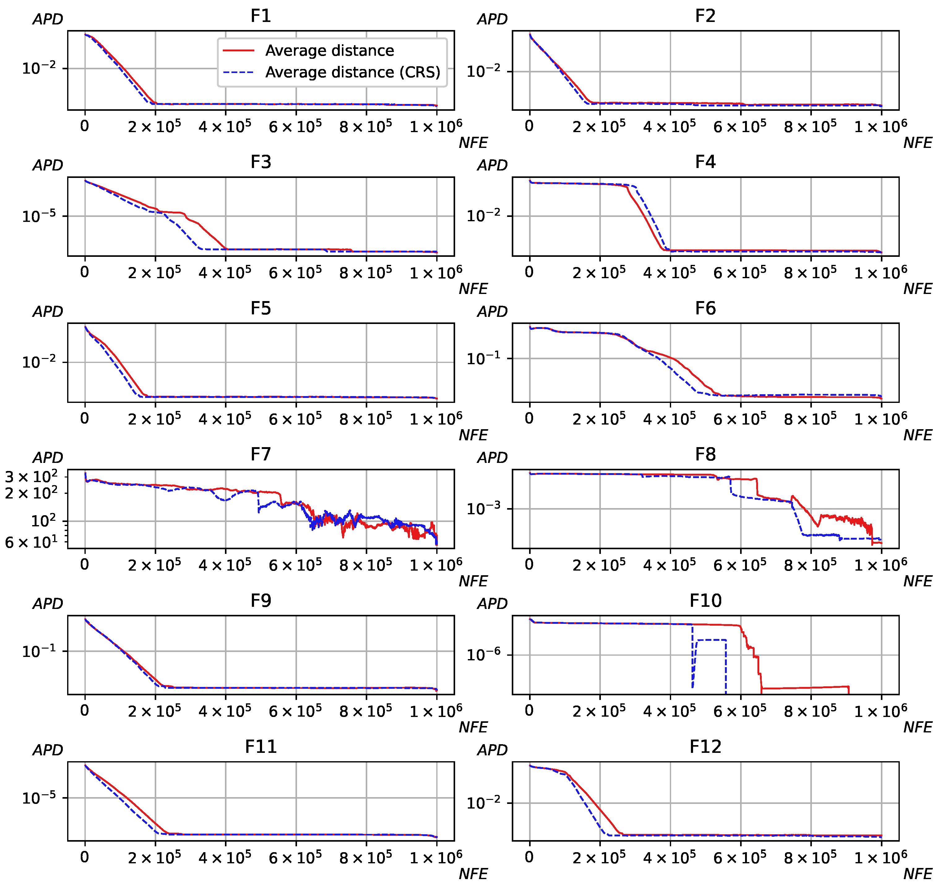
The presented comparison shows that there is a certain effect of the crossover rate sorting; however, it is important to understand the reasons for the algorithms’ different behaviors and convergence speeds. For this purpose, first of all, the diversity measure is introduced as the average pairwise distance ($APD$) between individuals:

$$APD=\frac{2}{N(N-1)}\sum _{i=1}^N\sum _{k=i+1}^N\sqrt{{\sum }_{j=1}^D{(x_{i,j}-x_{k,j})}^2}$$

(9)

Figure 2 shows the diversity of the newest population in the L-NTADE algorithm with and without crossover rate sorting (CRS), CEC 2022, $20\ast D$ case.

The graphs in Figure 2 demonstrate that applying crossover rate sorting results in earlier diversity loss in the population in most cases. The only exception here is F4, Shifted and Rotated Non-Continuous Rastrigin’s Function, where the diversity stays at a high level for a longer period. Hence, the improvement on the CEC 2022 benchmark can be explained by faster convergence. However, this convergence may be premature, for example, like on F10, where applying crossover rate sorting leads to early stop of the search process. Two other important cases are hybrid functions F7 and F8, where diversity oscillated, but here, it is also lower with CRS. Similar trends are observed for other algorithms in both CEC 2022 and CEC 2017 benchmarks.

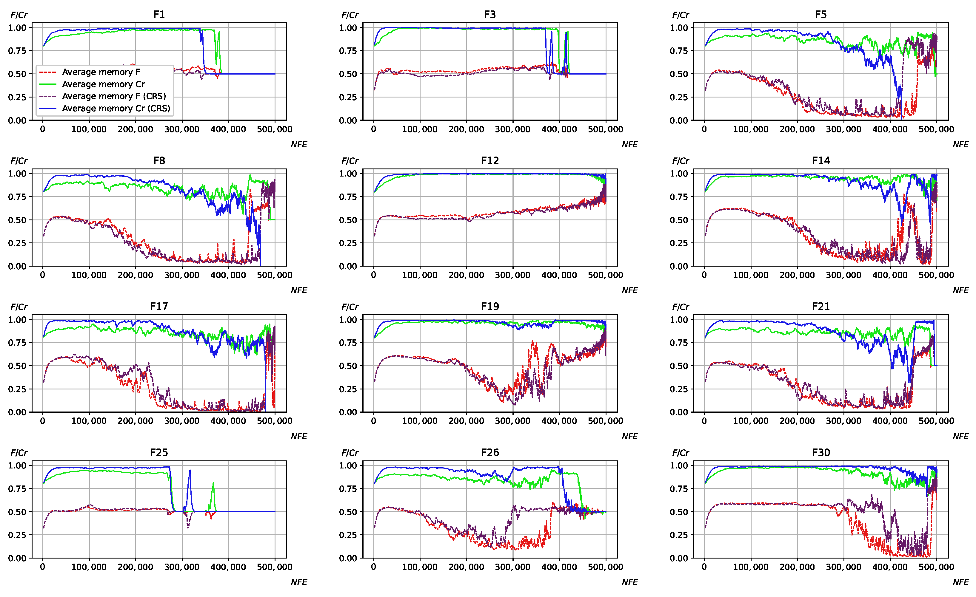
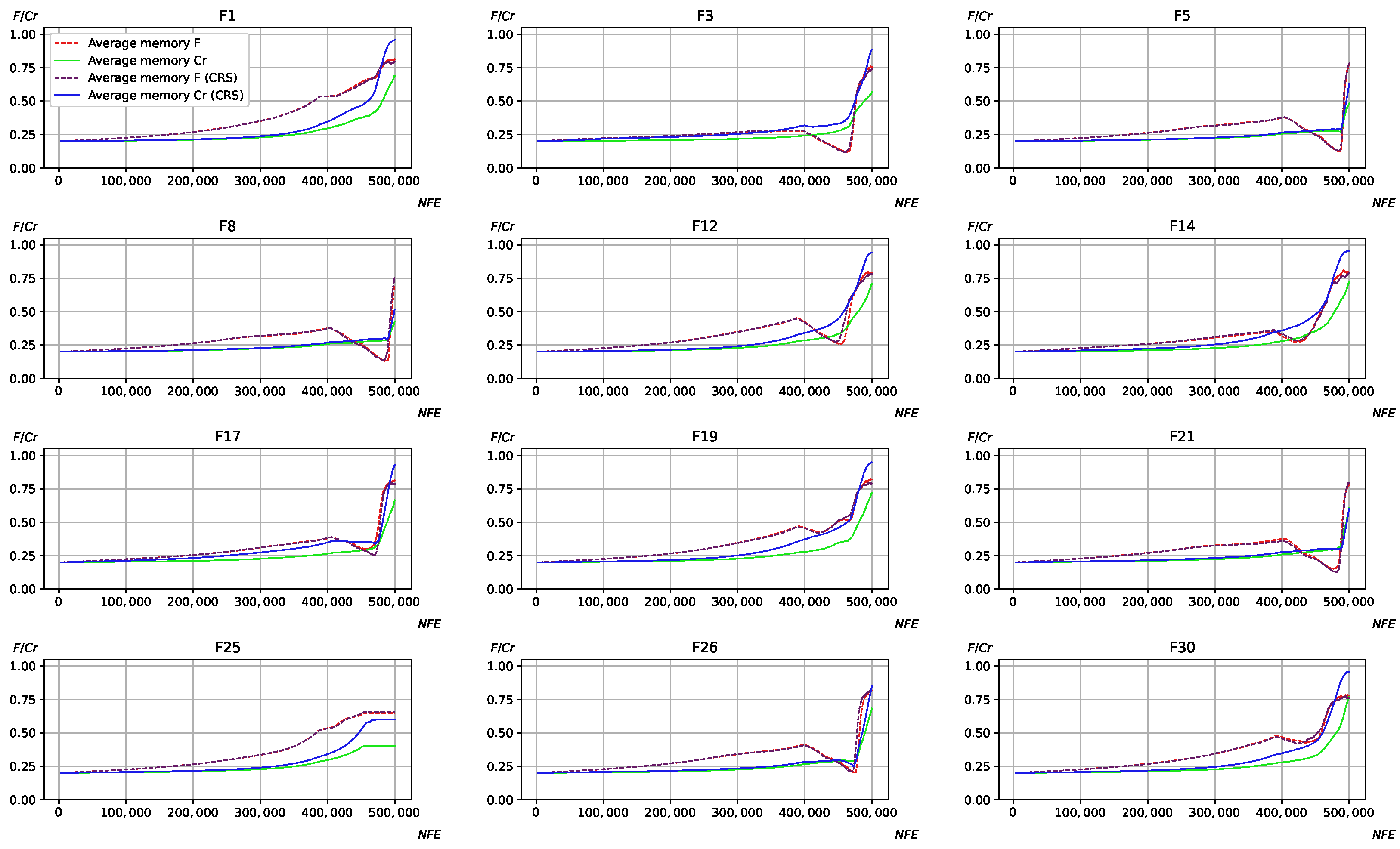
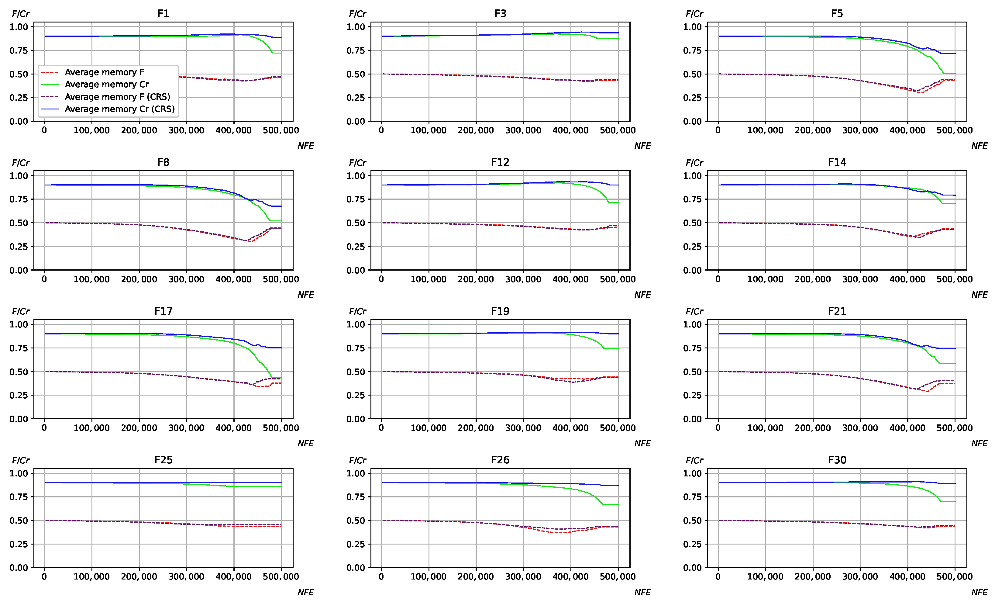
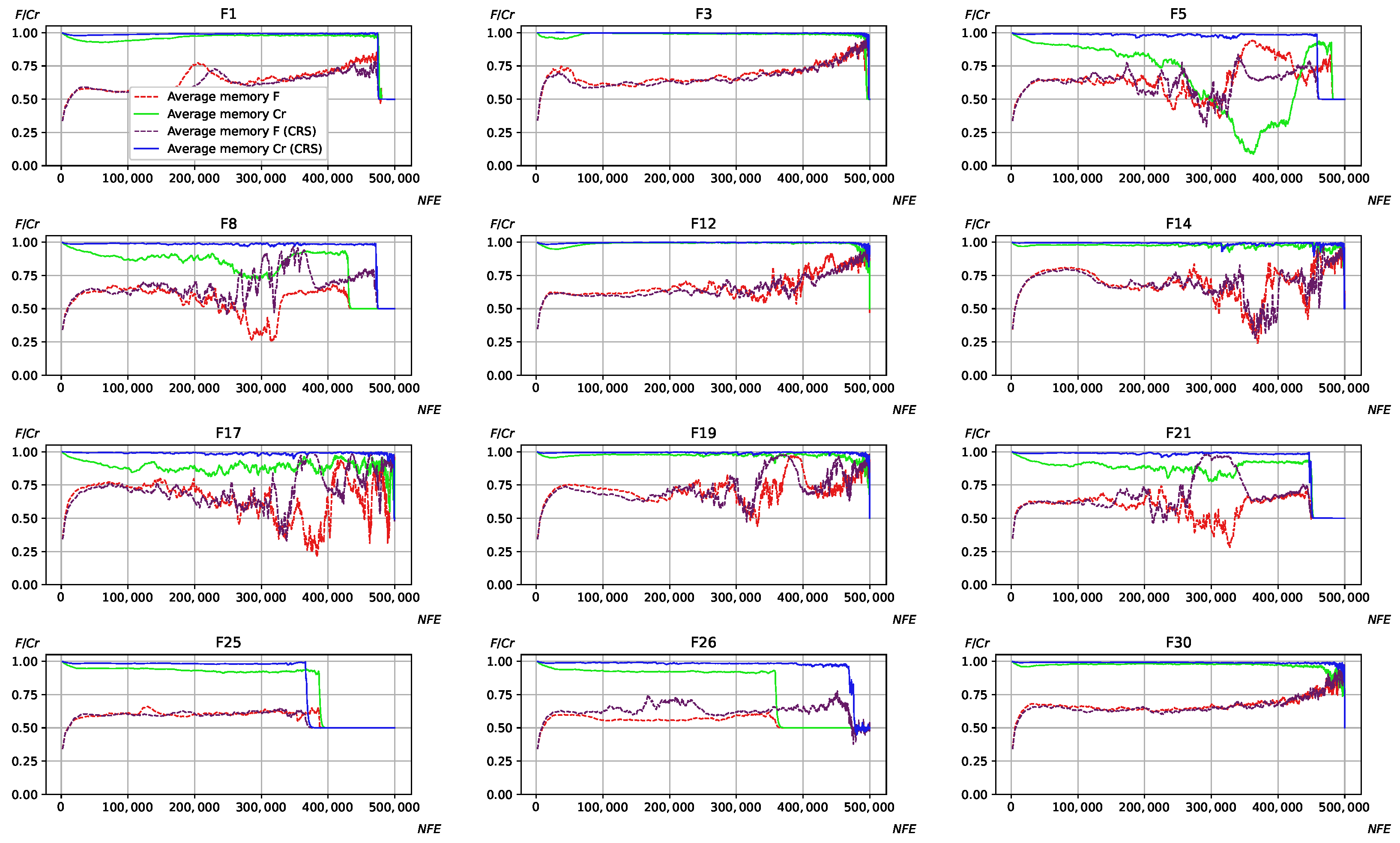
Another question worth investigating is the influence of crossover rate sorting on the process of parameter adaptation. For this purpose, the average values of all memory cells were calculated for F and $Cr$ for all algorithms. Figure 3, Figure 4, Figure 5 and Figure 6 show the adaptation process on CEC 2017, $50\ast D$ case.

Considering the results in Figure 3, Figure 4, Figure 5 and Figure 6, it can be observed that applying CRS results in larger $Cr$ values stored in the memory cells in the majority of cases. Moreover, $Cr$ often reaches 1, and rarely decreases, especially for L-SHADE-RSP and L-NTADE, where the memory size is rather small. The NL-SHADE-RSP is characterized by a more rapid increase in the average of the $Cr$ values in the memory cells, while L-SHADE-LBC keeps larger $Cr$ values for a longer period of time. The scaling factor parameter F is also affected, especially for the L-NTADE algorithm, where its behavior may differ significantly, e.g., in cases such as F8, F17, and F21. One explanation for this could be that decreased diversity leads to different F values to become more promising, usually resulting in larger F values in the memory cells.

The presented graphs may lead to the following question: is the faster convergence and larger $Cr$ values generated the only effects of the crossover rate sorting? Is it possible to achieve the same results simply by setting larger $Cr$ values, without any sorting? To answer these questions, another set of experiments was performed. In these experiments, the biased parameter adaptation approach [23] was applied; in particular, the Lehmer mean parameter p in memory cells update was increased. The standard setting for this parameter in L-SHADE-RSP, NL-SHADE-RSP and L-NTADE is 2, and it was increased to 4. In L-SHADE-LBC, this parameter is linearly controlled so that it is increased by 2. Larger values of p lead to a bias toward larger parameter values generated.

Table 5. Algorithms with crossover rate sorting and biased Lehmer mean, CEC 2017, Mann–Whitney tests and total standard score.

Algorithms	$10\ast \mathit{D}$	$30\ast \mathit{D}$	$50\ast \mathit{D}$	$100\ast \mathit{D}$
L-SHADE-RSP_lm vs.	1/28/1	7/22/1	7/22/1	5/23/2
L-SHADE-RSP_s	(2.05)	(29.73)	(36.46)	(23.53)
NL-SHADE-RSP_lm vs.	2/27/1	1/28/1	1/28/1	0/24/6
NL-SHADE-RSP_s	(12.63)	(4.82)	(−12.18)	(−22.63)
NL-SHADE-LBC_lm vs.	1/28/1	4/25/1	14/14/2	10/17/3
NL-SHADE-LBC_s	(−12.23)	(28.68)	(51.67)	(46.90)
L-NTADE_lm vs.	0/29/1	1/23/6	1/21/8	5/14/11
L-NTADE_s	(−2.67)	(−23.53)	(−32.82)	(−33.29)

and

Table 6. Algorithms with crossover rate sorting and biased Lehmer mean, CEC 2022, Mann–Whitney tests and total standard score.

Algorithms	$10\ast \mathit{D}$	$20\ast \mathit{D}$
L-SHADE-RSP_lm vs.	4/8/0	5/7/0
L-SHADE-RSP_s	(27.64)	(26.19)
NL-SHADE-RSP_lm vs.	4/7/1	3/9/0
NL-SHADE-RSP_s	(12.52)	(12.86)
NL-SHADE-LBC_lm vs.	6/6/0	5/7/0
NL-SHADE-LBC_s	(35.73)	(29.54)
L-NTADE_lm vs.	4/8/0	3/7/2
L-NTADE_s	(22.77)	(13.21)

show the comparison of the four used algorithm with the increased Lehmer mean parameter (with _lm in the name) and with crossover rate sorting on CEC 2017 and CEC 2022, respectively.

Comparing Table 1 and Table 5, it can be noted that in terms of number of wins/ties/losses, applying the biased Lehmer mean does not change the situation in most cases. However, the performance of NL-SHADE-RSP in high-dimensional problems is increased, and the algorithm with crossover rate sorting becomes much worse, especially in $100\ast D$. Similar trends are observed for CEC 2022 in Table reftab6, where a significant difference may be observed for NL-SHADE-RSP in the $10\ast D$ case—here adding more biased mean calculation leads to more similar performance to NL-SHADE-RSP_s, in terms of convergence speed.

Table 7. Algorithms with crossover rate sorting vs. alternative approaches, CEC 2017, Mann–Whitney tests and total standard score.

Algorithms	$10\ast \mathit{D}$	$30\ast \mathit{D}$	$50\ast \mathit{D}$	$100\ast \mathit{D}$
LSHADE-RSP_s vs.	8/15/7	8/13/9	6/10/14	6/7/17
LSHADE-SPACMA	(−0.72)	(−16.83)	(−62.19)	(−83.76)
LSHADE-RSP_s vs.	0/28/2	5/20/5	12/14/4	18/9/3
jSO	(−9.76)	(6.64)	(42.59)	(101.81)
LSHADE-RSP_s vs.	3/15/12	10/9/11	10/8/12	11/15/4
EBOwithCMAR	(−53.67)	(−24.75)	(6.79)	(47.58)
NL-SHADE-RSP_s vs.	11/7/12	3/4/23	0/2/28	0/0/30
LSHADE-SPACMA	(−5.52)	(−163.45)	(−241.37)	(−257.55)
NL-SHADE-RSP_s vs.	9/8/13	3/4/23	0/1/29	1/0/29
jSO	(−22.72)	(−160.24)	(−237.64)	−239.21)
NL-SHADE-RSP_s vs.	7/11/12	3/4/23	0/0/30	1/1/28
EBOwithCMAR	(−41.34)	(−155.81)	(−240.52)	−231.45)
NL-SHADE-LBC_s vs.	8/18/4	4/9/17	2/3/25	2/1/27
LSHADE-SPACMA	(10.80)	(−106.52)	(−185.40)	(−202.37)
NL-SHADE-LBC_s vs.	4/22/4	1/8/21	2/2/26	3/2/25
jSO	(−3.88)	(−143.58)	(−178.59)	(−174.86)
NL-SHADE-LBC_s vs.	2/19/9	1/10/19	2/3/25	2/2/26
EBOwithCMAR	(−56.85)	(−127.87)	(−164.10)	(−176.55)
L-NTADE_s vs.	8/12/10	13/8/9	12/3/15	11/3/16
LSHADE-SPACMA	(−26.36)	(18.21)	(−14.62)	(−45.39)
L-NTADE_s vs.	7/12/11	11/12/7	16/10/4	18/4/8
jSO	(−37.93)	(30.81)	(83.28)	(73.70)
L-NTADE_s vs.	3/16/11	11/13/6	17/5/8	13/5/12
EBOwithCMAR	(−54.66)	(25.78)	(49.77)	(31.42)

shows the comparison of algorithms with crossover rate sorting with some of the top-performing algorithms, such as EBOwithCMAR [36] (first place in 2017), jSO [7] (second place) and LSHADE-SPACMA [37] (fourth place) on the CEC 2017 benchmark.

Table 8. Algorithms with crossover rate sorting vs. alternative approaches, CEC 2022, Mann–Whitney tests and total standard score.

Algorithms	$10\ast \mathit{D}$	$20\ast \mathit{D}$
LSHADE-RSP_s vs.	2/3/7	5/3/4
EA4eigN100_10	(−36.18)	(5.54)
LSHADE-RSP_s vs.	4/2/6	6/2/4
NL-SHADE-RSP-MID	(−7.53)	(16.98)
LSHADE-RSP_s vs.	7/1/4	9/1/2
APGSK-IMODE	(28.48)	(49.20)
NL-SHADE-RSP_s vs.	1/2/9	2/1/9
EA4eigN100_10	(−54.42)	(−51.07)
NL-SHADE-RSP_s vs.	2/4/6	1/5/6
NL-SHADE-RSP-MID	(−27.32)	(−27.73)
NL-SHADE-RSP_s vs.	7/2/3	5/2/5
APGSK-IMODE	(18.97)	(3.82)
NL-SHADE-LBC_s vs.	5/3/4	5/3/4
EA4eigN100_10	(7.96)	(8.30)
NL-SHADE-LBC_s vs.	5/4/3	6/2/4
NL-SHADE-RSP-MID	(15.33)	(10.70)
NL-SHADE-LBC_s vs.	10/1/1	8/1/3
APGSK-IMODE	(58.57)	(38.79)
L-NTADE_s vs.	2/4/6	3/5/4
EA4eigN100_10	(−28.38)	(−3.66)
L-NTADE_s vs.	4/4/4	7/1/4
NL-SHADE-RSP-MID	(−3.38)	(16.63)
L-NTADE_s vs.	7/3/2	10/0/2
APGSK-IMODE	(37.75)	(51.52)

contains the comparison on the CEC 2022 benchmark with EA4eigN100_10 [38] (first place in competition), NL-SHADE-RSP-MID [39] (third place in competition) and APGSK-IMODE [40].

The statistical test results are shown in Table 7; it can be seen that NL-SHADE-RSP and NL-SHADE-LBC algorithms did not perform well on this benchmark, as they were designed for CEC 2021 and CEC 2022 benchmarks. However, the L-SHADE-RSP_s was able to outperform the EBOwithCMAR and jSO in high-dimensional problems, despite losing several times in low-dimensional cases. As for the L-NTADE_s, its performance is also good, and it won against EBOwithCMAR and jSO in $30\ast D$, $50\ast D$ and $100\ast D$, despite performing worse than L-SHADE-SPACMA.

In the case of the CEC 2022 benchmark, shown in Table 8, the L-SHADE-RSP_s performed quite well, even in comparison with the best methods in the $20\ast D$ problems, but showed worse results in $10\ast D$, unlike NL-SHADE-RSP_s, which had worse performance. The NL-SHADE-LBC with crossover rate sorting showed similar performance compared to the top algorithms, and the L-NTADE_s was worse in the $10\ast D$ case but comparable in $20\ast D$. It is important to note here that the L-NTADE_s is capable of achieving high performance in both CEC 2017 and CEC 2022 benchmarks against different algorithms developed for these problem sets.

4. Discussion

The results presented in the previous section show that applying sorting of the crossover rate values has a significant effect on the diversity of the population, convergence speed and even parameter adaptation of modern adaptive differential evolution. The reason for the lower diversity is that assigning larger crossover rate parameter values $Cr$ to worse individuals leads to potentially larger changes in them. In other words, worse individuals are changed more significantly and hence are faster driven toward better objective function values. This, in turn, has two major effects. Firstly, the diversity is decreased faster, and secondly, larger crossover rate values receive higher improvements, resulting in larger $Cr$ in memory cells. The second effect also leads to larger $Cr$ values being assigned also to the best individuals in the population, compared to the same algorithm without crossover rate sorting.

All the described effects of the sorting $Cr$ values are not always positive and depend on the algorithm used. For example, in the performed experiments on the CEC 2017 benchmark, where the computational resource is rather small, dimensions are high, and problems are diverse, applying sorting in L-SHADE-RSP and L-SHADE-LBC gives a positive effect, while NL-SHADE-RSP and L-NTADE show decreased performance as the dimension increases. In the case of the CEC 2022 benchmark, where the convergence speed is important, sorting $Cr$ results in increased performance for all algorithms. An additional experiment with increased bias in parameter adaptation showed that sorting is not the same as simply increasing the generated $Cr$ values, and it has a more complicated effect on the differential evolution performance. In general, a similar sorting could be applied to other parameters and algorithms. However, the preliminary experiments with scaling factor F sorting did not show any performance improvements, even though the tests were performed with sorting in ascending and descending order. Nevertheless, some other approaches, such as genetic algorithms, which use parameter adaptation, may benefit from sorting generated parameter values, although aspect this requires additional studies.

5. Conclusions

In this study, the crossover rate sorting mechanism was investigated and applied to four adaptive differential evolution algorithms. It was shown that it is capable of improving the performance of DE in many cases, and it is not equal to the increase in crossover rate values. Sorting crossover rates results in faster convergence but also diversity loss, and hence should be carefully applied in adaptive differential evolution. Nevertheless, as the experiments showed, the negative effects on the algorithm performance are quite limited, so sorting can be included in the differential evolution algorithm. Further studies in this direction many include developing specific parameter adaptation mechanisms that consider the effects of sorting. For example, the parameter adaptation for crossover rates can be excluded with $Cr$ values only generated by normal distribution with a mean value of 1—it was observed that this actually happens for some algorithms and does not cause significant performance problems.

References

1. Storn, R.; Price, K. Differential evolution—A simple and efficient heuristic for global optimization over continuous spaces. J. Glob. Optim. 1997, 11, 341–359. [Google Scholar] [CrossRef]
2. Qin, A.; Suganthan, P. Self-adaptive differential evolution algorithm for numerical optimization. In Proceedings of the IEEE Congress on Evolutionary Computation, Edinburgh, UK, 2–5 September 2005; pp. 1785–1791. [Google Scholar] [CrossRef]
3. Brest, J.; Greiner, S.; Boškovic, B.; Mernik, M.; Žumer, V. Self-adapting control parameters in differential evolution: A comparative study on numerical benchmark problems. IEEE Trans. Evol. Comput. 2006, 10, 646–657. [Google Scholar] [CrossRef]
4. Zhang, J.; Sanderson, A.C. JADE: Self-adaptive differential evolution with fast and reliable convergence performance. In Proceedings of the 2007 IEEE Congress on Evolutionary Computation, Singapore, 25–28 September 2007; pp. 2251–2258. [Google Scholar]
5. Tanabe, R.; Fukunaga, A. Success-history based parameter adaptation for differential evolution. In Proceedings of the IEEE Congress on Evolutionary Computation, Cancun, Mexico, 20–23 June 2013; IEEE Press: Piscataway, NJ, USA, 2013; pp. 71–78. [Google Scholar] [CrossRef] [Green Version]
6. Wu, G.; Mallipeddi, R.; Suganthan, P.N.; Wang, R.; Chen, H. Differential evolution with multi-population based ensemble of mutation strategies. Inf. Sci. 2016, 329, 329–345. [Google Scholar] [CrossRef]
7. Brest, J.; Maučec, M.; Boškovic, B. Single objective real-parameter optimization algorithm jSO. In Proceedings of the IEEE Congress on Evolutionary Computation, San Sebastian, Spain, 5–8 June 2017; IEEE Press: Piscataway, NJ, USA, 2017; pp. 1311–1318. [Google Scholar] [CrossRef]
8. Das, S.; Suganthan, P. Differential evolution: A survey of the state-of-the-art. IEEE Trans. Evol. Comput. 2011, 15, 4–31. [Google Scholar] [CrossRef]
9. Das, S.; Mullick, S.; Suganthan, P. Recent advances in differential evolution—An updated survey. Swarm Evol. Comput. 2016, 27, 1–30. [Google Scholar] [CrossRef]
10. Bilal; Pant, M.; Zaheer, H.; García-Hernández, L.; Abraham, A. Differential Evolution: A review of more than two decades of research. Eng. Appl. Artif. Intell. 2020, 90, 103479. [Google Scholar] [CrossRef]
11. Ahmad, M.F.; Isa, N.A.; Lim, W.H.; Ang, K.M. Differential evolution: A recent review based on state-of-the-art works. Alex. Eng. J. 2021, 61, 3831–3872. [Google Scholar] [CrossRef]
12. Zhou, Y.-Z.; Yi, W.-C.; Gao, L.; Li, X.-Y. Adaptive differential evolution with sorting crossover rate for continuous optimization problems. IEEE Trans. Cybern. 2017, 47, 2742–2753. [Google Scholar] [CrossRef] [PubMed]
13. Stanovov, V.; Akhmedova, S.; Semenkin, E. LSHADE Algorithm with Rank-Based Selective Pressure Strategy for Solving CEC 2017 Benchmark Problems. In Proceedings of the 2018 IEEE Congress on Evolutionary Computation (CEC), Rio de Janeiro, Brazil, 8–13 July 2018; pp. 1–8. [Google Scholar] [CrossRef]
14. Stanovov, V.; Akhmedova, S.; Semenkin, E. NL-SHADE-RSP Algorithm with Adaptive Archive and Selective Pressure for CEC 2021 Numerical Optimization. In Proceedings of the 2021 IEEE Congress on Evolutionary Computation (CEC), Krakow, Poland, 28 June–1 July 2021; pp. 809–816. [Google Scholar] [CrossRef]
15. Stanovov, V.; Akhmedova, S.; Semenkin, E. NL-SHADE-LBC algorithm with linear parameter adaptation bias change for CEC 2022 Numerical Optimization. In Proceedings of the 2022 IEEE Congress on Evolutionary Computation (CEC), Padua, Italy, 18–23 July 2022. [Google Scholar] [CrossRef]
16. Stanovov, V.; Akhmedova, S.; Semenkin, E. Dual-Population Adaptive Differential Evolution Algorithm L-NTADE. Mathematics 2022, 10, 4666. [Google Scholar] [CrossRef]
17. Awad, N.; Ali, M.; Liang, J.; Qu, B.; Suganthan, P. Problem Definitions and Evaluation Criteria for the CEC 2017 Special Session and Competition on Single Objective Bound Constrained Real-Parameter Numerical Optimization; Technical Report; Nanyang Technological University: Singapore, 2016. [Google Scholar]
18. Kumar, A.; Price, K.; Mohamed, A.K.; Suganthan, P.N. Problem Definitions and Evaluation Criteria for the CEC 2022 Special Session and Competition on Single Objective Bound Constrained Numerical Optimization; Technical Report; Nanyang Technological University: Singapore, 2021. [Google Scholar]
19. Price, K.; Storn, R.; Lampinen, J. Differential Evolution: A Practical Approach to Global Optimization; Springer: Berlin/Heidelberg, Germany, 2005. [Google Scholar]
20. Kitamura, T.; Fukunaga, A. Duplicate Individuals in Differential Evolution. In Proceedings of the 2022 IEEE Congress on Evolutionary Computation (CEC), Padua, Italy, 18–23 July 2022. [Google Scholar] [CrossRef]
21. Kumar, A.; Biswas, P.P.; Suganthan, P.N. Differential evolution with orthogonal array-based initialization and a novel selection strategy. Swarm Evol. Comput. 2022, 68, 101010. [Google Scholar] [CrossRef]
22. Al-Dabbagh, R.D.; Neri, F.; Idris, N.; Baba, M.S.B. Algorithmic design issues in adaptive differential evolution schemes: Review and taxonomy. Swarm Evol. Comput. 2018, 43, 284–311. [Google Scholar] [CrossRef]
23. Stanovov, V.; Akhmedova, S.; Semenkin, E. Biased Parameter Adaptation in Differential Evolution. Inf. Sci. 2021, 566, 215–238. [Google Scholar] [CrossRef]
24. Stanovov, V.; Akhmedova, S.; Semenkin, E. The automatic design of parameter adaptation techniques for differential evolution with genetic programming. Knowl. Based Syst. 2022, 239, 108070. [Google Scholar] [CrossRef]
25. Stanovov, V.; Akhmedova, S.; Semenkin, E. Neuroevolution for parameter adaptation in differential evolution. Algorithms 2022, 15, 122. [Google Scholar] [CrossRef]
26. Tanabe, R.; Fukunaga, A. Improving the search performance of SHADE using linear population size reduction. In Proceedings of the IEEE Congress on Evolutionary Computation, CEC, Beijing, China, 6–11 July 2014; pp. 1658–1665. [Google Scholar] [CrossRef] [Green Version]
27. Stanovov, V.; Akhmedova, S.; Semenkin, E. Visualizing Crossover Rate Influence in Differential Evolution with Expected Fitness Improvement. In Proceedings of the Metaheuristics and Nature Inspired Computing: 8th International Conference, META 2021, Marrakech, Morocco, 27–30 October 2021; Springer: Cham, Swizterland, 2022; p. 1541. [Google Scholar] [CrossRef]
28. Gong, W.; Cai, Z.; Wang, Y. Repairing the crossover rate in adaptive differential evolution. Appl. Soft Comput. 2014, 15, 149–168. [Google Scholar] [CrossRef]
29. Cai, Z.; Wang, Y. Differential evolution with hybrid linkage crossover. Inf. Sci. 2015, 320, 244–287. [Google Scholar] [CrossRef]
30. Deng, L.; Wang, S.; Qiao, L.; Zhang, B. DE-RCO: Rotating Crossover Operator With Multiangle Searching Strategy for Adaptive Differential Evolution. IEEE Access 2018, 6, 2970–2983. [Google Scholar] [CrossRef]
31. Xu, Y.; Fang, J.; Zhu, W.; Wang, X.; Zhao, L. Differential evolution using a superior–inferior crossover scheme. Comput. Optim. Appl. 2015, 61, 243–274. [Google Scholar] [CrossRef]
32. Fan, Q.; Zhang, Y. Self-adaptive differential evolution algorithm with crossover strategies adaptation and its application in parameter estimation. Chemom. Intell. Lab. Syst. 2016, 151, 164–171. [Google Scholar] [CrossRef]
33. Sallam, K.M.; Elsayed, S.M.; Chakrabortty, R.K.; Ryan, M.J. Improved Multi-operator Differential Evolution Algorithm for Solving Unconstrained Problems. In Proceedings of the 2020 IEEE Congress on Evolutionary Computation (CEC), Glasgow, UK, 19–24 July 2020; pp. 1–8. [Google Scholar] [CrossRef]
34. Cheng, L.; Wang, Y.; Wang, C.; Mohamed, A.W.; Xiao, T. Adaptive Differential Evolution Based on Successful Experience Information. IEEE Access 2020, 8, 164611–164636. [Google Scholar] [CrossRef]
35. Kitamura, T.; Fukunaga, A. Differential Evolution with an Unbounded Population. In Proceedings of the 2022 IEEE Congress on Evolutionary Computation (CEC), Padua, Italy, 18–23 July 2022. [Google Scholar] [CrossRef]
36. Kumar, A.; Misra, R.K.; Singh, D. Improving the local search capability of Effective Butterfly Optimizer using Covariance Matrix Adapted Retreat Phase. In Proceedings of the IEEE Congress on Evolutionary Computation, Donostia, Spain, 5–8 June 2017; pp. 1835–1842. [Google Scholar] [CrossRef]
37. Mohamed, A.W.; Hadi, A.A.; Fattouh, A.M.; Jambi, K.M. LSHADE with semi-parameter adaptation hybrid with CMA-ES for solving CEC 2017 benchmark problems. In Proceedings of the IEEE Congress on Evolutionary Computation, Donostia, Spain, 5–8 June 2017; pp. 145–152. [Google Scholar] [CrossRef]
38. Bujok, P.; Kolenovsky, P. Eigen Crossover in Cooperative Model of Evolutionary Algorithms Applied to CEC 2022 Single Objective Numerical Optimisation. In Proceedings of the IEEE Congress on Evolutionary Computation, Padua, Italy, 18–23 July 2022; pp. 1–8. [Google Scholar] [CrossRef]
39. Biedrzycki, R.; Arabas, J.; Warchulski, E. A Version of NL-SHADE-RSP Algorithm with Midpoint for CEC 2022 Single Objective Bound Constrained Problems. In Proceedings of the IEEE Congress on Evolutionary Computation, Padua, Italy, 18–23 July 2022; pp. 1–8. [Google Scholar] [CrossRef]
40. Mohamed, A.W.; Hadi, A.A.; Agrawal, P.; Sallam, K.M.; Mohamed, A.K. Gaining-Sharing Knowledge Based Algorithm with Adaptive Parameters Hybrid with IMODE Algorithm for Solving CEC 2021 Benchmark Problems. In Proceedings of the IEEE Congress on Evolutionary Computation, Kraków, Poland, 28 June–1 July 2021; pp. 841–848. [Google Scholar] [CrossRef]
Figure 1. Block-scheme of the L-NTADE_s algorithm.
Algorithms 16 00133 g001
Figure 2. Average pairwise distance between individuals in the newest population, L-NTADE, CEC 2022, 20 D .
Algorithms 16 00133 g002
Figure 3. Parameter adaptation with and without crossover rate sorting, L-SHADE-RSP, CEC 2017, 50 D .
Algorithms 16 00133 g003
Figure 4. Parameter adaptation with and without crossover rate sorting, NL-SHADE-RSP, CEC 2017, 50 D .
Algorithms 16 00133 g004
Figure 5. Parameter adaptation with and without crossover rate sorting, NL-SHADE-LBC, CEC 2017, 50 D .
Algorithms 16 00133 g005
Figure 6. Parameter adaptation with and without crossover rate sorting, L-NTADE, CEC 2017, 50 D .
Algorithms 16 00133 g006