
The D-Bar Algorithm Fusing Electrical Impedance Tomography with A Priori Radar Data: A Hands-On Analysis


Abstract
1. Introduction
2. Fundamentals
2.1. Basic EIT Equations
2.2. D-Bar Algorithm
3. Numerical Implementation
3.1. Numerical Implementation of the D-Bar Algorithm
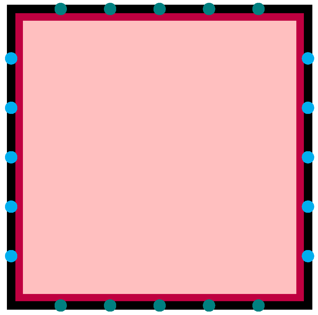
3.2. EIT Simulation Setup
3.3. Radar Simulation Setup
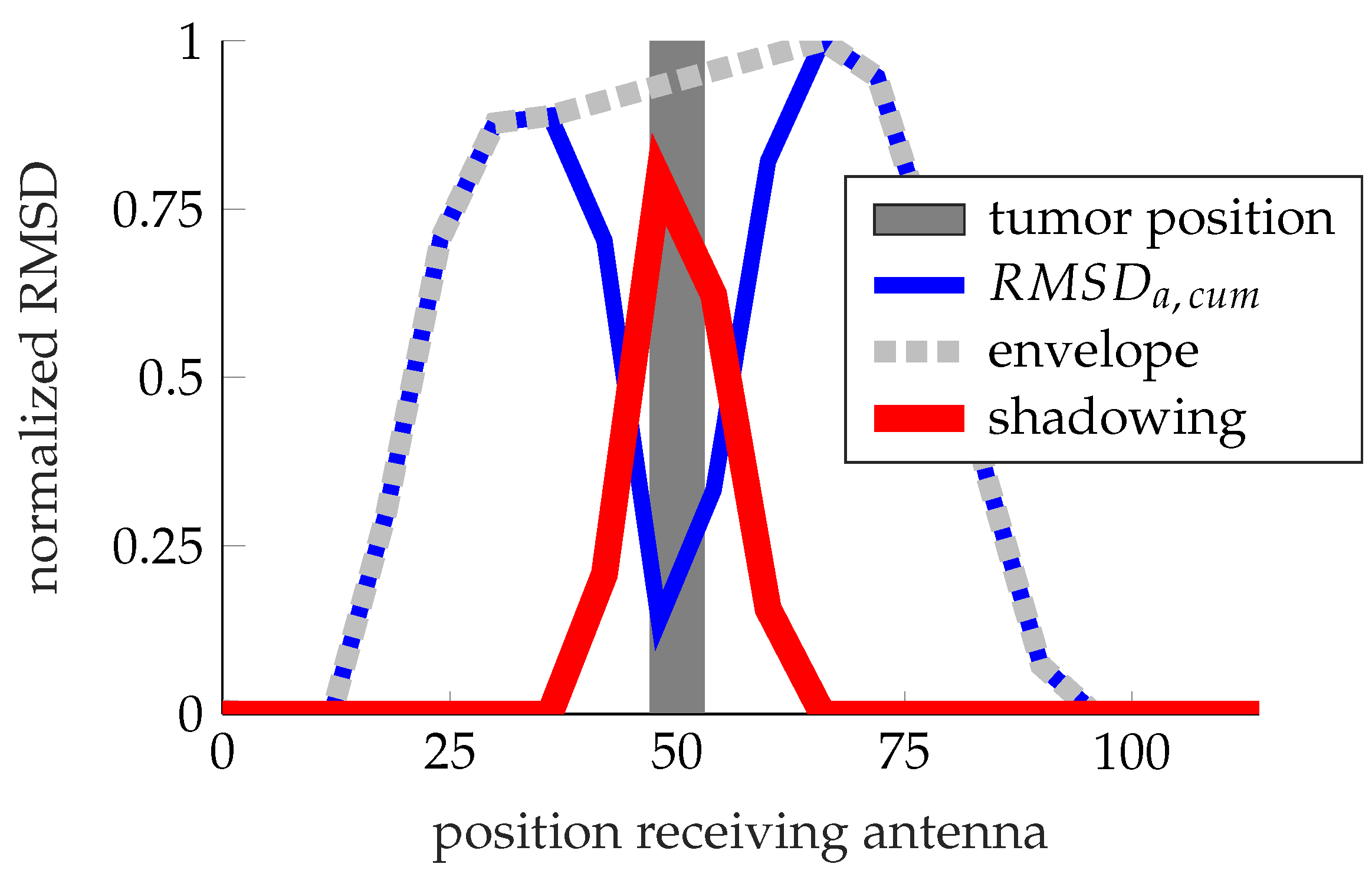
3.4. Radar Reconstruction
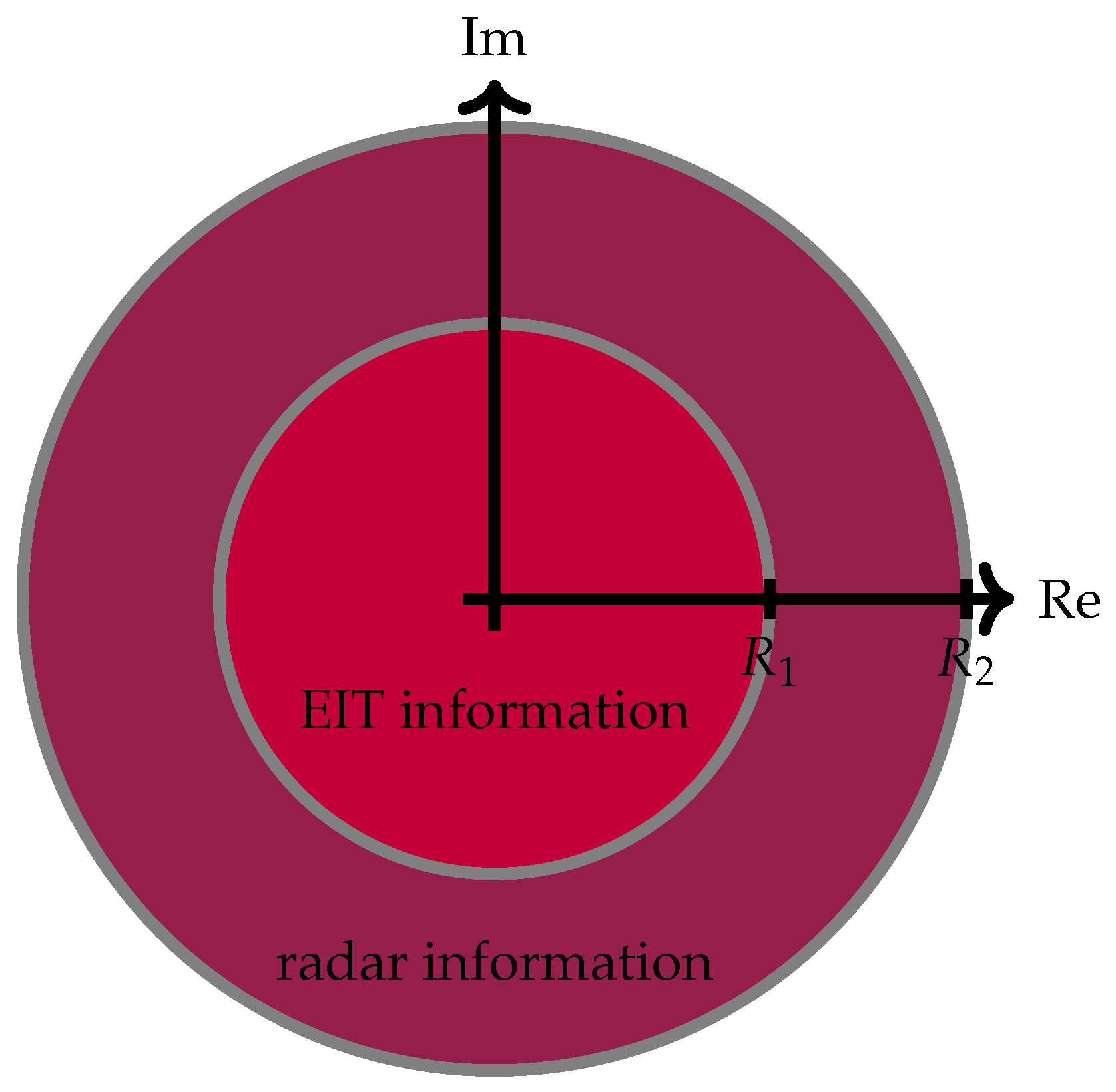
3.5. Fusion of EIT and Radar
3.6. Evaluation of the Reconstructions
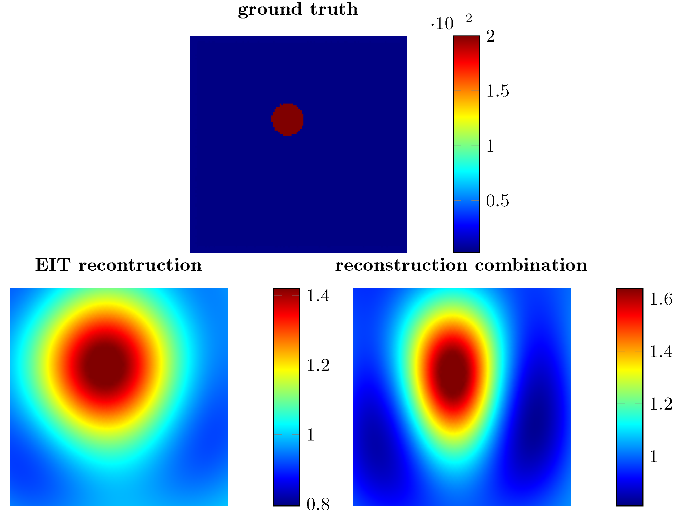
4. Results
5. Conclusions and Outlook
Supplementary Materials
Author Contributions
Funding
Data Availability Statement
Conflicts of Interest
Abbreviations
| EIT | Electrical impedance tomography |
| DN-map | Dirichlet-to-Neumann map |
| ND | Neumman-to-Dirichlet |
| RMSD | Root-mean-square deviation |
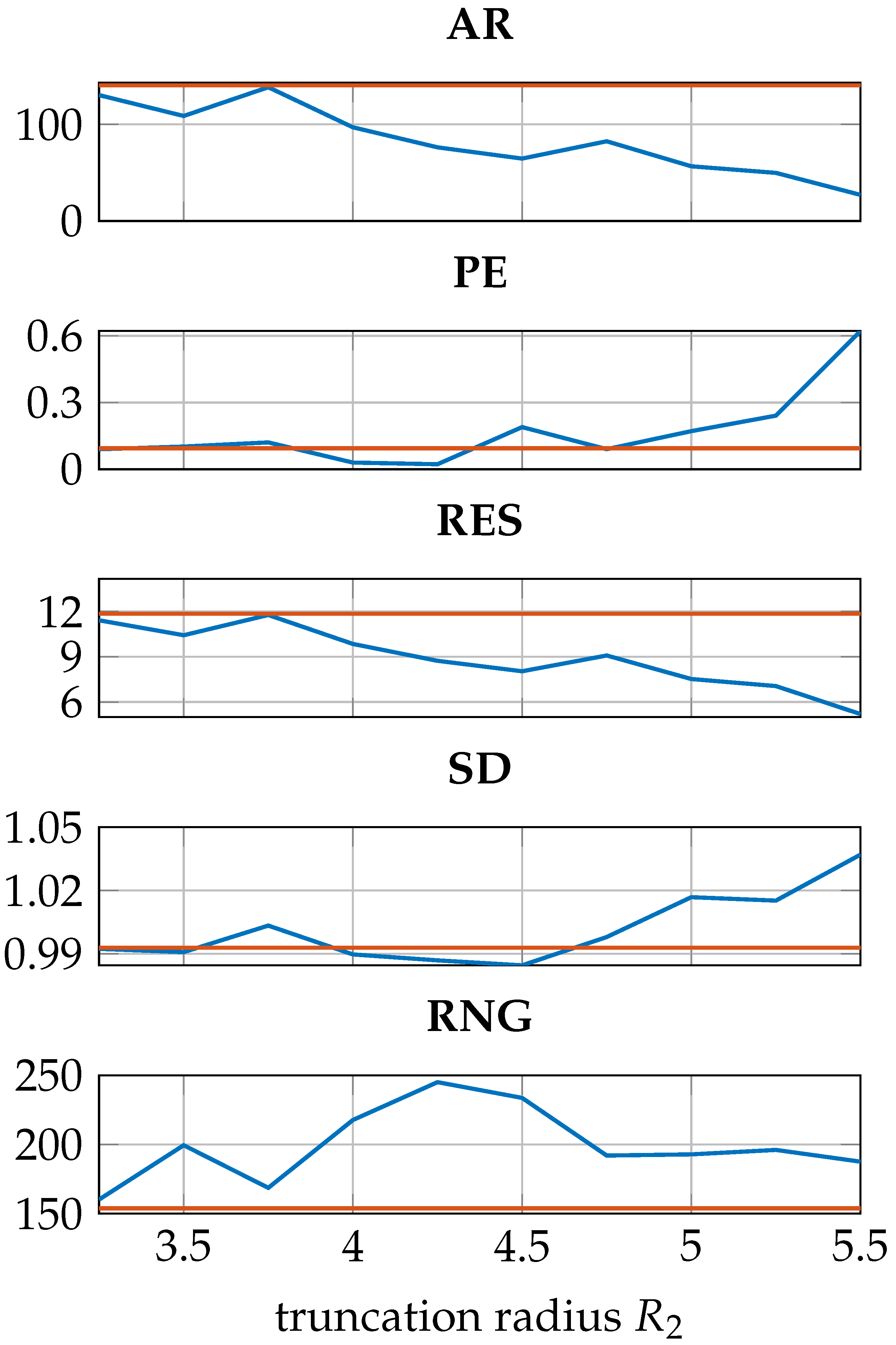
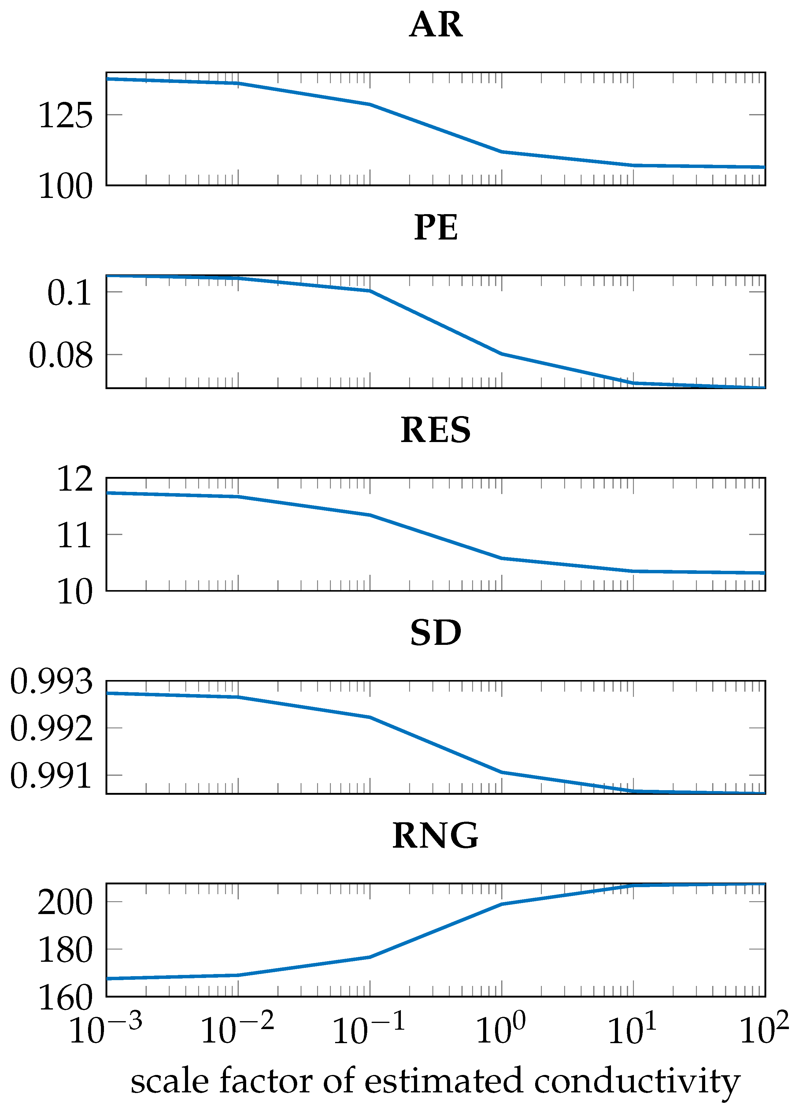
| AR | Amplitude response |
| PE | Position error |
| RES | Resolution |
| SD | Shape deformation |
| RNG | Ringing |
| CGO | Complex geometric optics |
Appendix A
Appendix A.1. D-Bar Algorithm
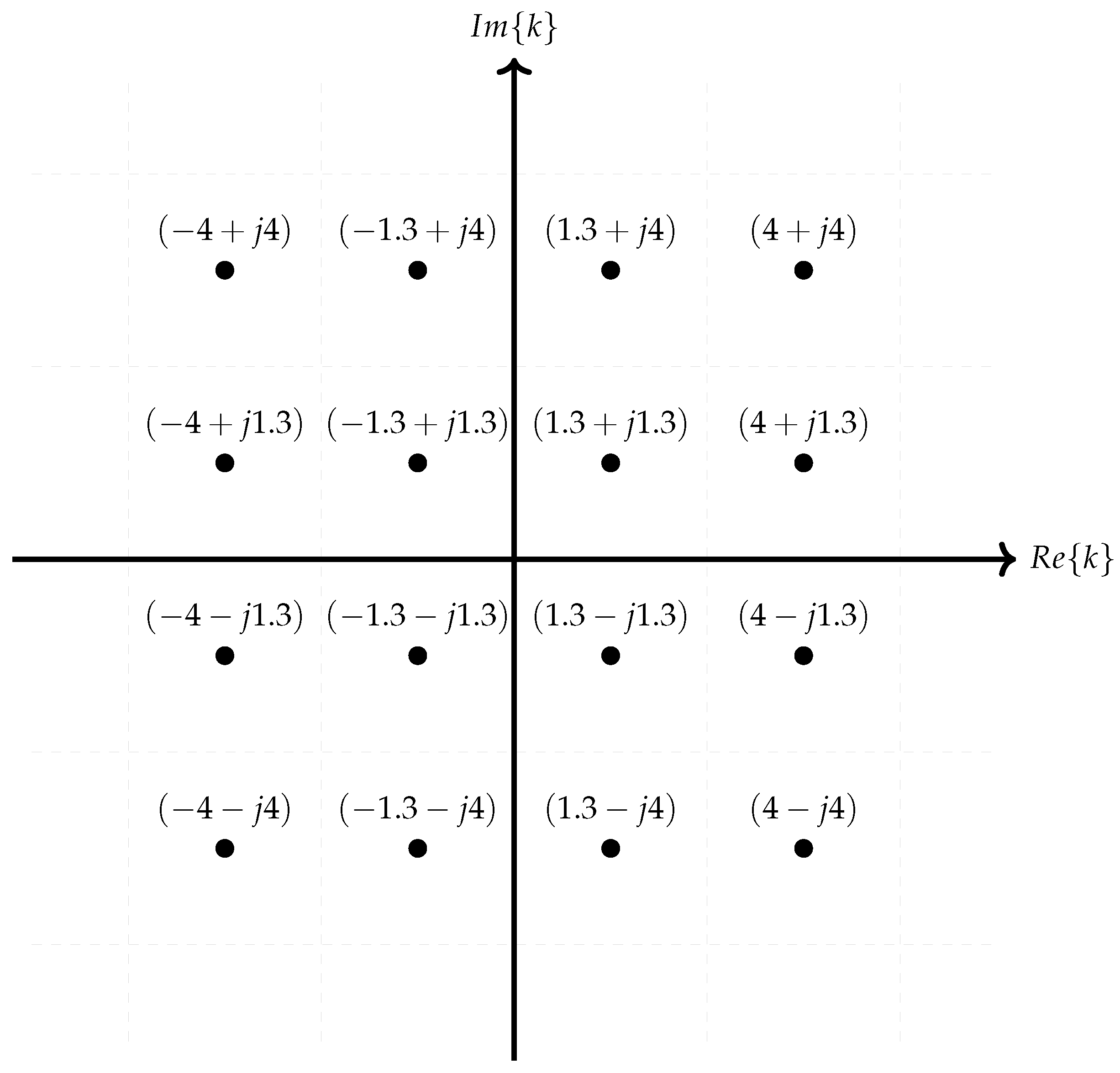
Appendix A.2. Sample of K

References
- Zhu, Q.; Lionheart, W.; Lidgey, F.; McLeod, C.; Paulson, K.; Pidcock, M. An adaptive current tomograph using voltage sources. IEEE Trans. Biomed. Eng. 1993, 40, 163–168. [Google Scholar] [CrossRef] [PubMed]
- Hentze, B.; Muders, T.; Luepschen, H.; Maripuu, E.; Hedenstierna, G.; Putensen, C.; Walter, M.; Leonhardt, S. Regional lung ventilation and perfusion by electrical impedance tomography compared to single-photon emission computed tomography. Physiol. Meas. 2018, 39, 065004. [Google Scholar] [CrossRef] [PubMed]
- Leonhardt, S.; Cordes, A.; Plewa, H.; Pikkemaat, R.; Soljanik, I.; Moehring, K.; Gerner, H.J.; Rupp, R. Electric impedance tomography for monitoring volume and size of the urinary bladder. Biomed. Eng./Biomed. Tech. 2011, 56, 301–307. [Google Scholar] [CrossRef] [PubMed]
- Meier, T.; Luepschen, H.; Karsten, J.; Leibecke, T.; Großherr, M.; Gehring, H.; Leonhardt, S. Assessment of regional lung recruitment and derecruitment during a PEEP trial based on electrical impedance tomography. Intensive Care Med. 2008, 34, 543–550. [Google Scholar] [CrossRef] [PubMed]
- Abascal, J.F.P.; Arridge, S.R.; Atkinson, D.; Horesh, R.; Fabrizi, L.; De Lucia, M.; Horesh, L.; Bayford, R.H.; Holder, D.S. Use of anisotropic modelling in electrical impedance tomography; description of method and preliminary assessment of utility in imaging brain function in the adult human head. Neuroimage 2008, 43, 258–268. [Google Scholar] [CrossRef]
- Hong, S.; Lee, K.; Ha, U.; Kim, H.; Lee, Y.; Kim, Y.; Yoo, H.J. A 4.9 mΩ-sensitivity mobile electrical impedance tomography IC for early breast-cancer detection system. IEEE J. Solid-State Circuits 2014, 50, 245–257. [Google Scholar] [CrossRef]
- Kruger, M.; Poolla, K.; Spanos, C.J. A class of impedance tomography based sensors for semiconductor manufacturing. In Proceedings of the 2004 American Control Conference, Boston, MA, USA, 30 June–2 July 2004; Volume 3, pp. 2178–2183. [Google Scholar]
- Hallaji, M.; Seppänen, A.; Pour-Ghaz, M. Electrical impedance tomography-based sensing skin for quantitative imaging of damage in concrete. Smart Mater. Struct. 2014, 23, 085001. [Google Scholar] [CrossRef]
- Vauhkonen, M.; Vadasz, D.; Karjalainen, P.A.; Somersalo, E.; Kaipio, J.P. Tikhonov regularization and prior information in electrical impedance tomography. IEEE Trans. Med. Imaging 1998, 17, 285–293. [Google Scholar] [CrossRef]
- Borsic, A.; Graham, B.M.; Adler, A.; Lionheart, W.R. Total Variation Regularization in Electrical Impedance Tomography; University of Manchester: Manchester, UK, 2007. [Google Scholar]
- Kaipio, J.P.; Kolehmainen, V.; Somersalo, E.; Vauhkonen, M. Statistical inversion and Monte Carlo sampling methods in electrical impedance tomography. Inverse Probl. 2000, 16, 1487. [Google Scholar] [CrossRef]
- Ahmad, S.; Strauss, T.; Kupis, S.; Khan, T. Comparison of statistical inversion with iteratively regularized Gauss Newton method for image reconstruction in electrical impedance tomography. Appl. Math. Comput. 2019, 358, 436–448. [Google Scholar] [CrossRef]
- Isaacson, D.; Mueller, J.L.; Newell, J.C.; Siltanen, S. Reconstructions of chest phantoms by the D-bar method for electrical impedance tomography. IEEE Trans. Med. Imaging 2004, 23, 821–828. [Google Scholar] [CrossRef]
- Calderón, A.P. On an inverse boundary value problem. Comput. Appl. Math 2006, 25, 133–138. [Google Scholar] [CrossRef]
- Nachman, A.I. Global uniqueness for a two-dimensional inverse boundary value problem. Ann. Math. 1996, 143, 71–96. [Google Scholar] [CrossRef]
- Siltanen, S.; Mueller, J.; Isaacson, D. An implementation of the reconstruction algorithm of A Nachman for the 2D inverse conductivity problem. Inverse Probl. 2000, 16, 681. [Google Scholar] [CrossRef]
- Murphy, E.K.; Mueller, J.L. Effect of domain shape modeling and measurement errors on the 2-D D-bar method for EIT. IEEE Trans. Med. Imaging 2009, 28, 1576–1584. [Google Scholar] [CrossRef]
- Sun, B.; Yue, S.; Hao, Z.; Cui, Z.; Wang, H. An improved Tikhonov regularization method for lung cancer monitoring using electrical impedance tomography. IEEE Sens. J. 2019, 19, 3049–3057. [Google Scholar] [CrossRef]
- Adler, A.; Lionheart, W.R. Uses and abuses of EIDORS: An extensible software base for EIT. Physiol. Meas. 2006, 27, S25. [Google Scholar] [CrossRef]
- Soleimani, M. Electrical impedance tomography imaging using a priori ultrasound data. Biomed. Eng. Online 2006, 5, 8. [Google Scholar] [CrossRef]
- Alsaker, M.; Mueller, J.L. A D-bar algorithm with a priori information for 2-dimensional electrical impedance tomography. SIAM J. Imaging Sci. 2016, 9, 1619–1654. [Google Scholar] [CrossRef]
- Hamilton, S.J.; Mueller, J.L.; Alsaker, M. Incorporating a Spatial Prior into Nonlinear D-Bar EIT Imaging for Complex Admittivities. IEEE Trans. Med. Imaging 2017, 36, 457–466. [Google Scholar] [CrossRef]
- Adler, A.; Gaggero, P.; Maimaitijiang, Y. Distinguishability in EIT using a hypothesis-testing model. J. Phys. Conf. Ser. 2010, 224, 012056. [Google Scholar] [CrossRef]
- Prati, M.V.; Moll, J.; Kexel, C.; Nguyen, D.H.; Santra, A.; Aliverti, A.; Krozer, V.; Issakov, V. Breast cancer imaging using a 24 GHz ultra-wideband MIMO FMCW radar: System considerations and first imaging results. In Proceedings of the 2020 14th European Conference on Antennas and Propagation (EuCAP), Copenhagen, Denmark, 15–20 March 2020; pp. 1–5. [Google Scholar]
- Flores-Tapia, D.; Pistorius, S. Electrical impedance tomography reconstruction using a monotonicity approach based on a priori knowledge. In Proceedings of the 2010 Annual International Conference of the IEEE Engineering in Medicine and Biology, Buenos Aires, Argentina, 31 August–4 September 2010; pp. 4996–4999. [Google Scholar]
- Cheney, M.; Isaacson, D. Issues in electrical impedance imaging. IEEE Comput. Sci. Eng. 1995, 2, 53–62. [Google Scholar] [CrossRef]
- Astala, K.; Päivärinta, L. Calderón’s inverse conductivity problem in the plane. Ann. Math. 2006, 163, 265–299. [Google Scholar] [CrossRef]
- Mueller, J.L.; Siltanen, S. Linear and Nonlinear Inverse Problems with Practical Applications; SIAM: Philadelphia, PA, USA, 2012. [Google Scholar]
- Herrera, C.N.; Vallejo, M.F.; Mueller, J.L.; Lima, R.G. Direct 2-D reconstructions of conductivity and permittivity from EIT data on a human chest. IEEE Trans. Med. Imaging 2014, 34, 267–274. [Google Scholar] [CrossRef] [PubMed]
- Dodd, M.; Mueller, J.L. A real-time D-bar algorithm for 2-D electrical impedance tomography data. Inverse Probl. Imaging 2014, 8, 1013. [Google Scholar] [CrossRef]
- Saad, Y.; Schultz, M.H. GMRES: A generalized minimal residual algorithm for solving nonsymmetric linear systems. SIAM J. Sci. Stat. Comput. 1986, 7, 856–869. [Google Scholar] [CrossRef]
- Gabriel, S.; Lau, R.; Gabriel, C. The dielectric properties of biological tissues: III. Parametric models for the dielectric spectrum of tissues. Phys. Med. Biol. 1996, 41, 2271. [Google Scholar] [CrossRef]
- Surowiec, A.J.; Stuchly, S.S.; Barr, J.R.; Swarup, A. Dielectric properties of breast carcinoma and the surrounding tissues. IEEE Trans. Biomed. Eng. 1988, 35, 257–263. [Google Scholar] [CrossRef]
- Martellosio, A.; Pasian, M.; Bozzi, M.; Perregrini, L.; Mazzanti, A.; Svelto, F.; Summers, P.E.; Renne, G.; Preda, L.; Bellomi, M. Dielectric properties characterization from 0.5 to 50 GHz of breast cancer tissues. IEEE Trans. Microw. Theory Tech. 2016, 65, 998–1011. [Google Scholar] [CrossRef]
- Mueller, J.L.; Siltanen, S. The d-bar method for electrical impedance tomography—Demystified. Inverse Probl. 2020, 36, 093001. [Google Scholar] [CrossRef]
- Adler, A.; Arnold, J.H.; Bayford, R.; Borsic, A.; Brown, B.; Dixon, P.; Faes, T.J.; Frerichs, I.; Gagnon, H.; Gärber, Y.; et al. GREIT: A unified approach to 2D linear EIT reconstruction of lung images. Physiol. Meas. 2009, 30, S35. [Google Scholar] [CrossRef]
- Alsaker, M.; Mueller, J.L. Use of an optimized spatial prior in D-bar reconstructions of EIT tank data. Inverse Probl. Imaging 2018, 12, 883. [Google Scholar] [CrossRef]
- Faddeev, L.D. Increasing solutions of the Schrödinger equation. Sov. Phys. Dokl. 1966, 10, 1033. [Google Scholar]


Disclaimer/Publisher’s Note: The statements, opinions and data contained in all publications are solely those of the individual author(s) and contributor(s) and not of MDPI and/or the editor(s). MDPI and/or the editor(s) disclaim responsibility for any injury to people or property resulting from any ideas, methods, instructions or products referred to in the content. |
© 2023 by the authors. Licensee MDPI, Basel, Switzerland. This article is an open access article distributed under the terms and conditions of the Creative Commons Attribution (CC BY) license (https://creativecommons.org/licenses/by/4.0/).
Share and Cite
Rixen, J.; Leonhardt, S.; Moll, J.; Nguyen, D.H.; Ngo, C. The D-Bar Algorithm Fusing Electrical Impedance Tomography with A Priori Radar Data: A Hands-On Analysis. Algorithms 2023, 16, 43. https://doi.org/10.3390/a16010043
Rixen J, Leonhardt S, Moll J, Nguyen DH, Ngo C. The D-Bar Algorithm Fusing Electrical Impedance Tomography with A Priori Radar Data: A Hands-On Analysis. Algorithms. 2023; 16(1):43. https://doi.org/10.3390/a16010043
Chicago/Turabian StyleRixen, Jöran, Steffen Leonhardt, Jochen Moll, Duy Hai Nguyen, and Chuong Ngo. 2023. "The D-Bar Algorithm Fusing Electrical Impedance Tomography with A Priori Radar Data: A Hands-On Analysis" Algorithms 16, no. 1: 43. https://doi.org/10.3390/a16010043
APA StyleRixen, J., Leonhardt, S., Moll, J., Nguyen, D. H., & Ngo, C. (2023). The D-Bar Algorithm Fusing Electrical Impedance Tomography with A Priori Radar Data: A Hands-On Analysis. Algorithms, 16(1), 43. https://doi.org/10.3390/a16010043