

Evolutionary Algorithm with Geometrical Heuristics for Solving the Close Enough Traveling Salesman Problem: Application to the Trajectory Planning of an Unmanned Aerial Vehicle

Abstract
1. Introduction
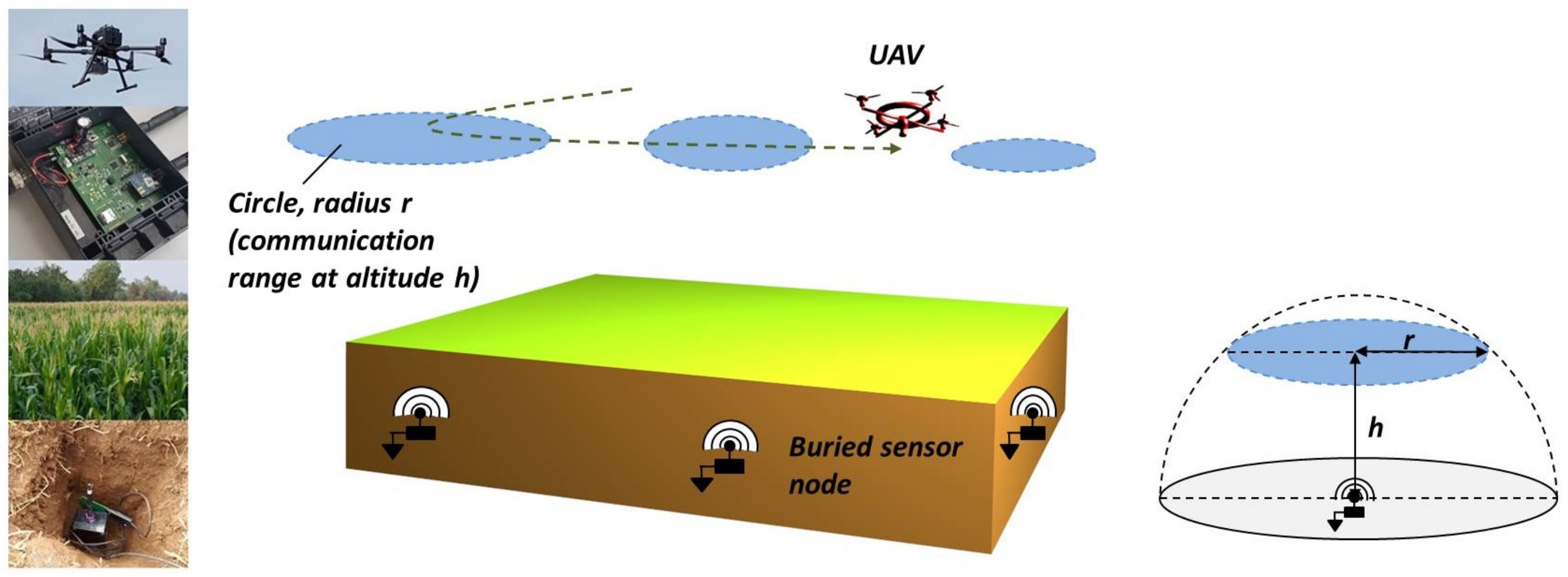
1.1. Application and Objective
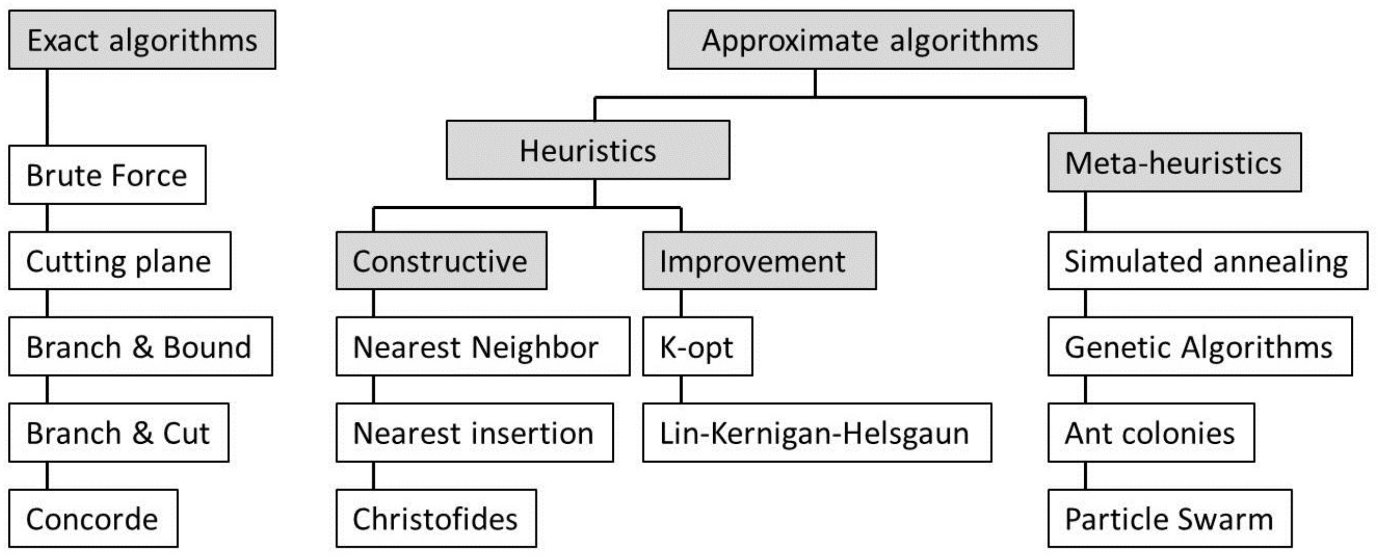
1.2. Related Works
1.3. Contributions and Paper Organization
2. Methodology
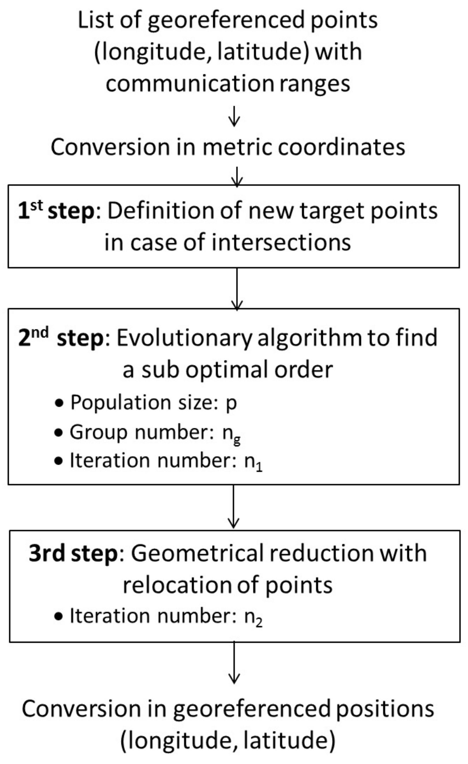
2.1. Modeling and Methodology Proposed
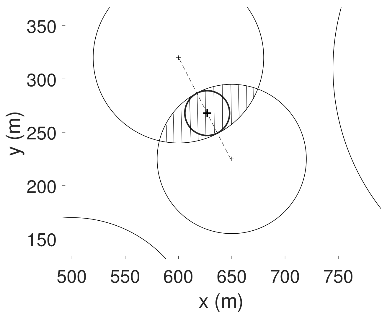
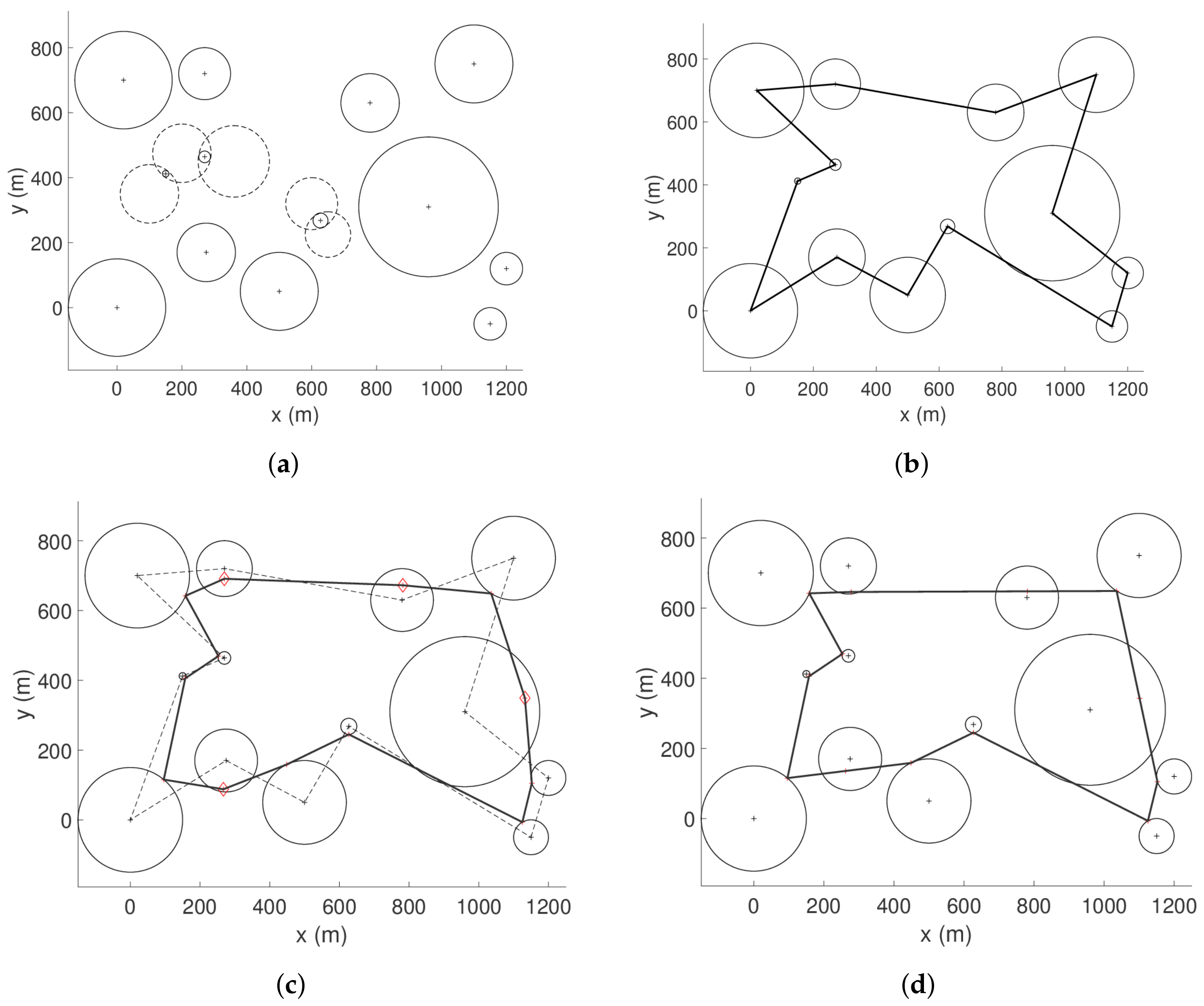
2.2. First Step: New Target Locations in Case of Intersections
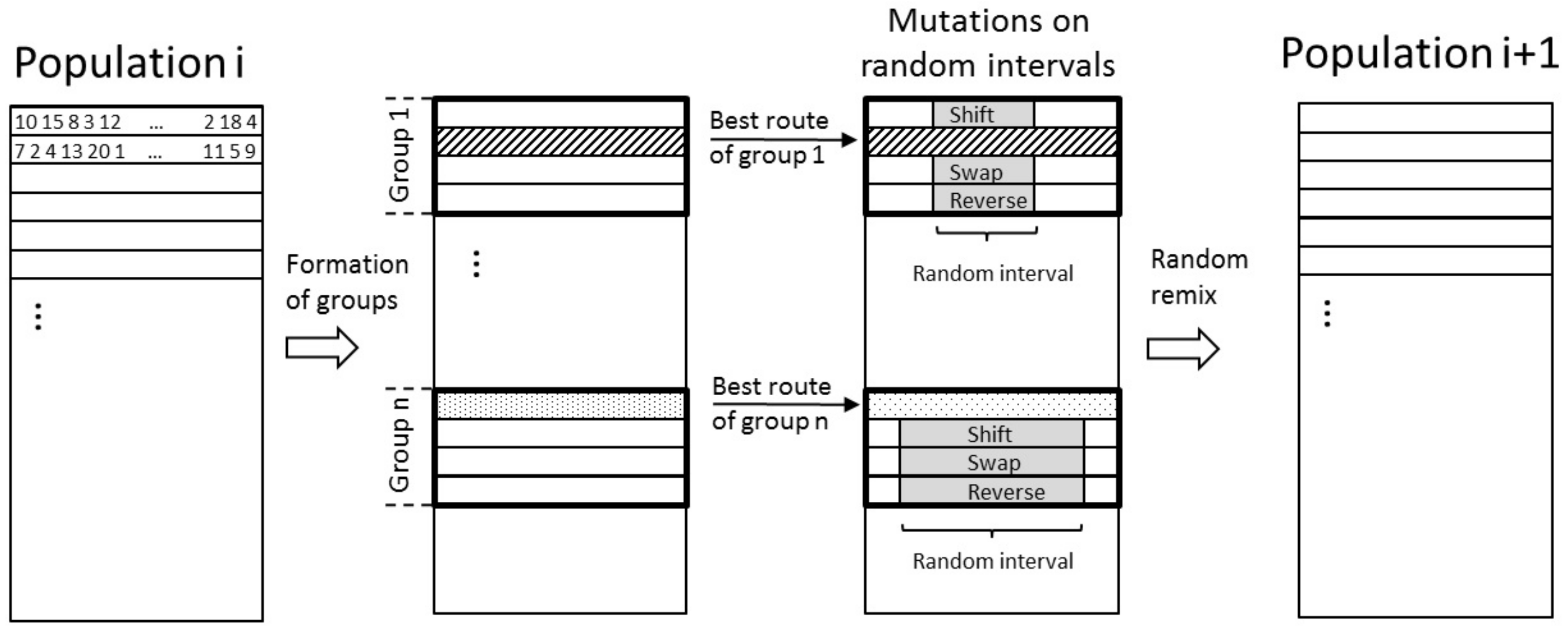
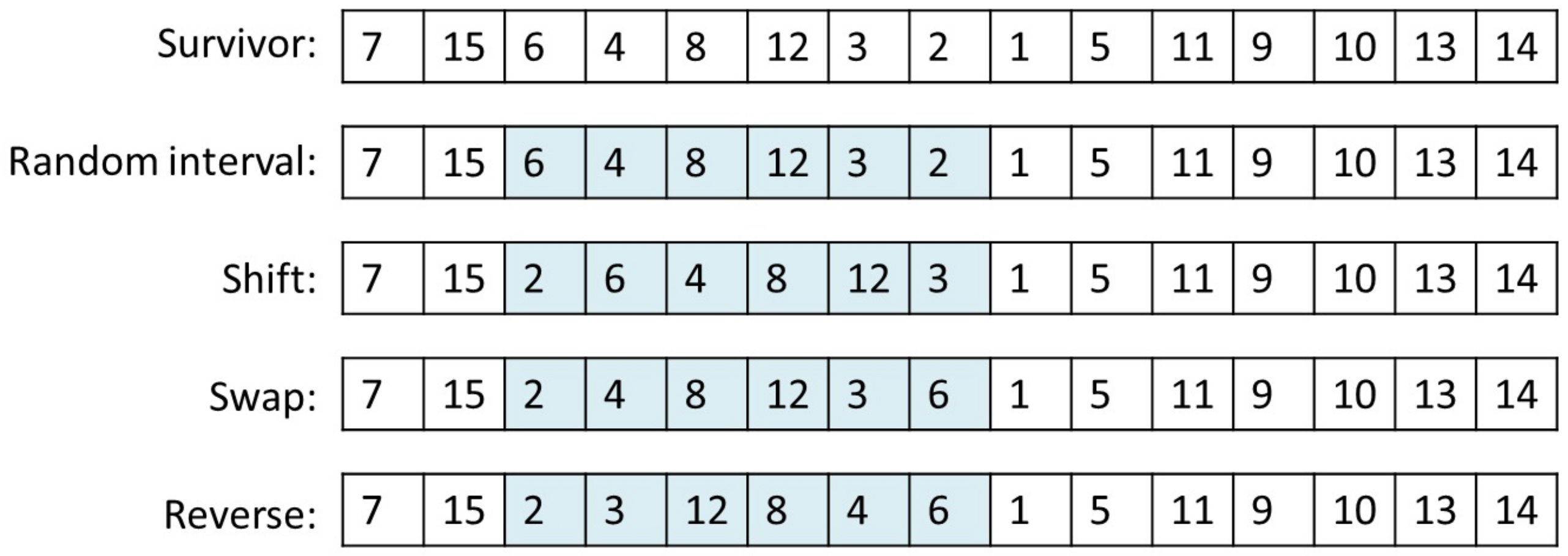
2.3. Second Step: Evolutionary Algorithm to Find a Sub Optimal Order
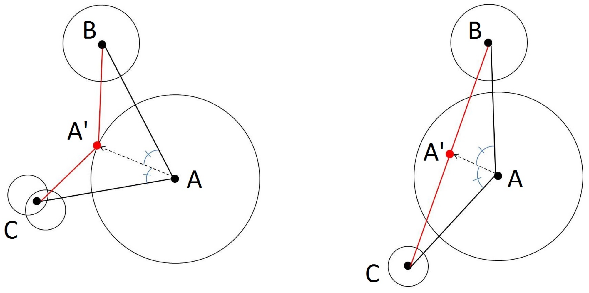
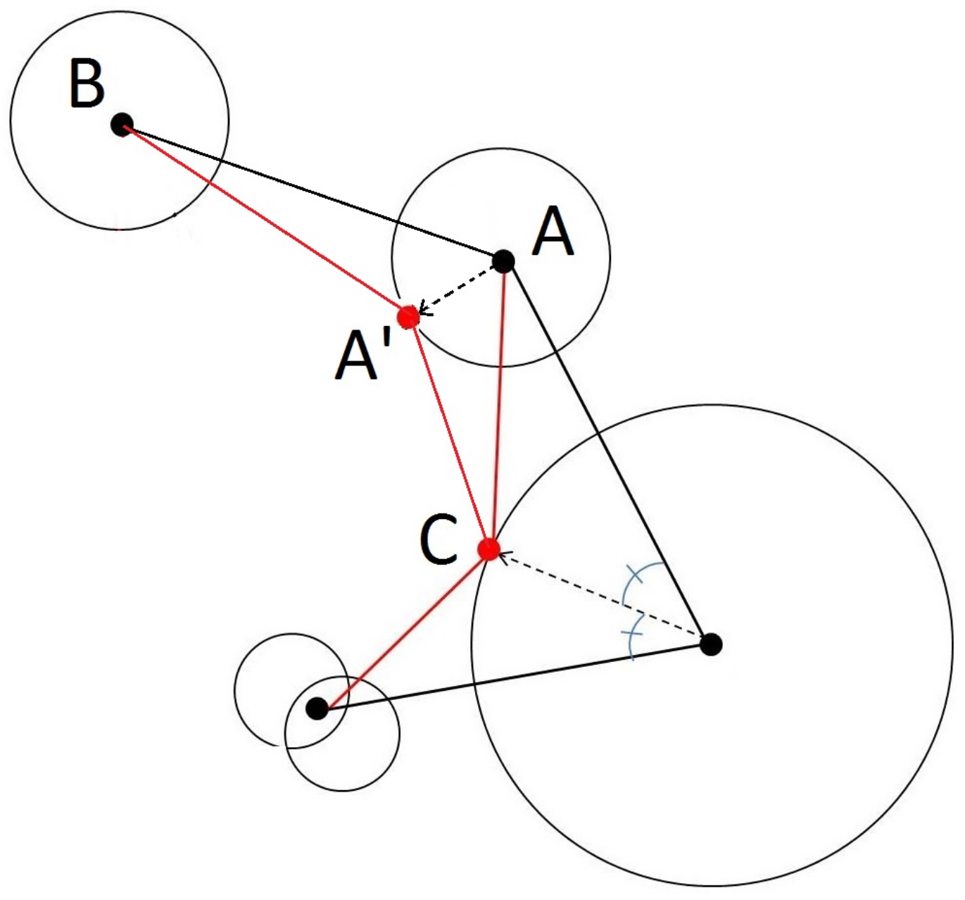
2.4. Step 3: Geometrical Reduction
3. Results
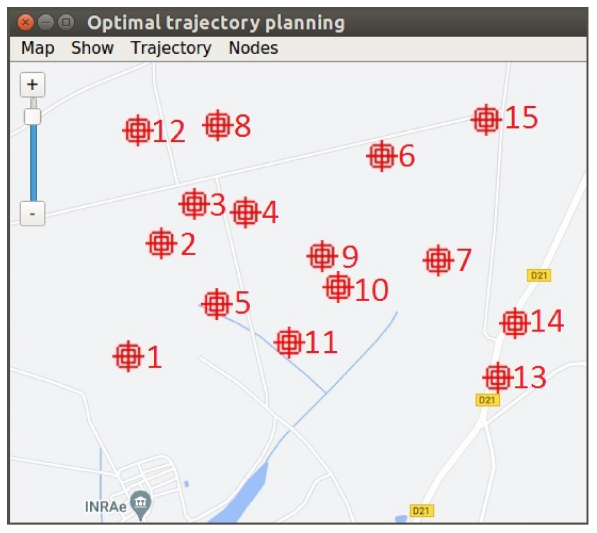
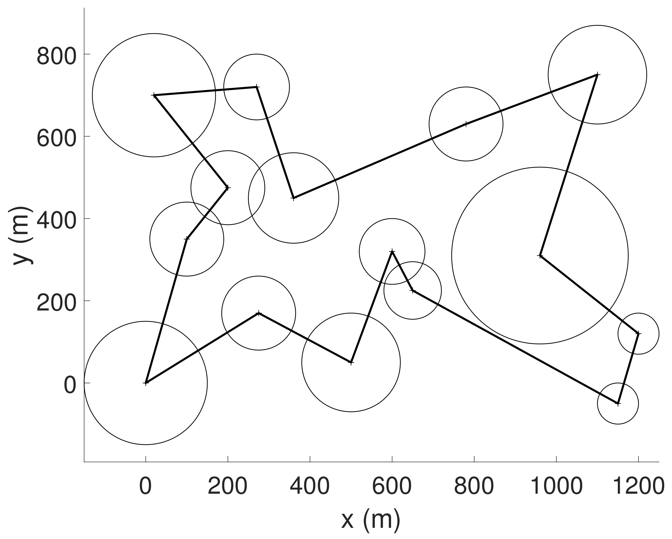
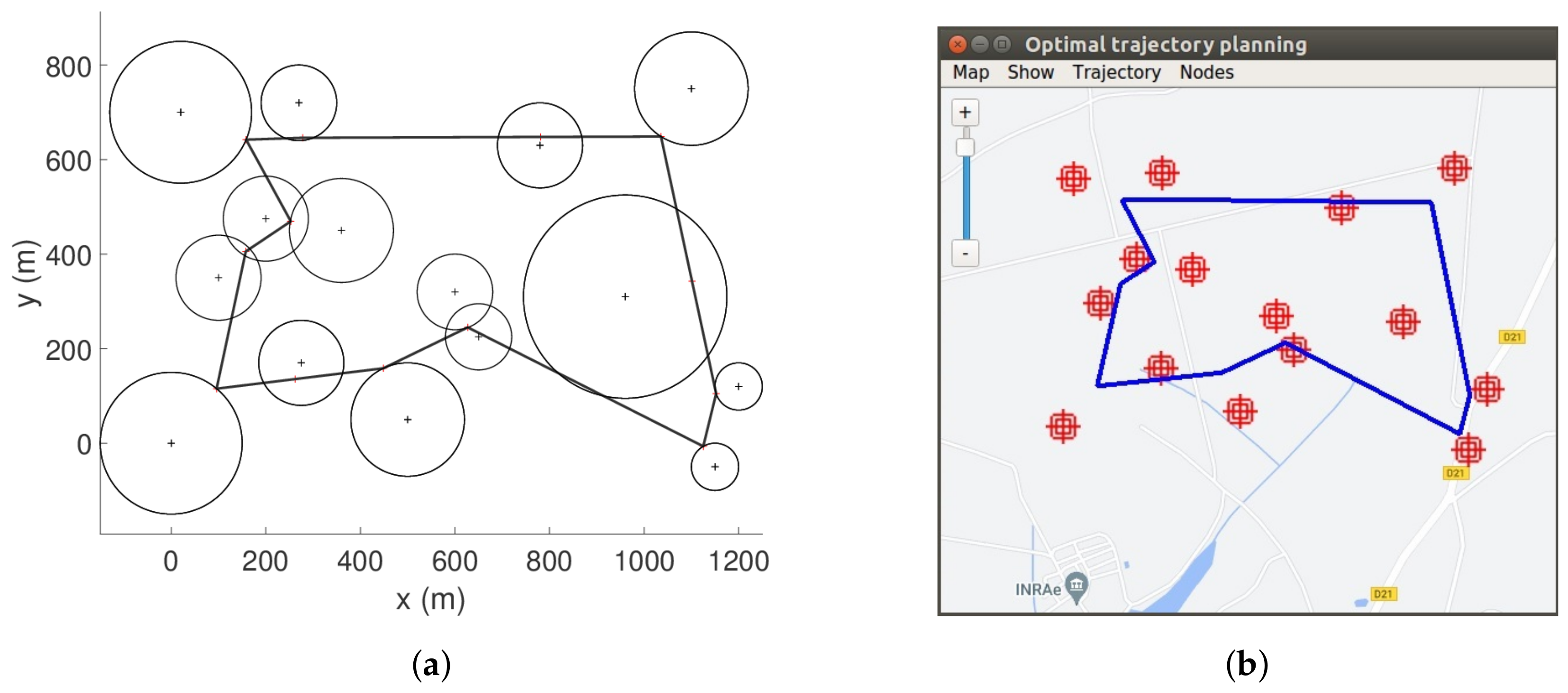
3.1. Preliminary Test
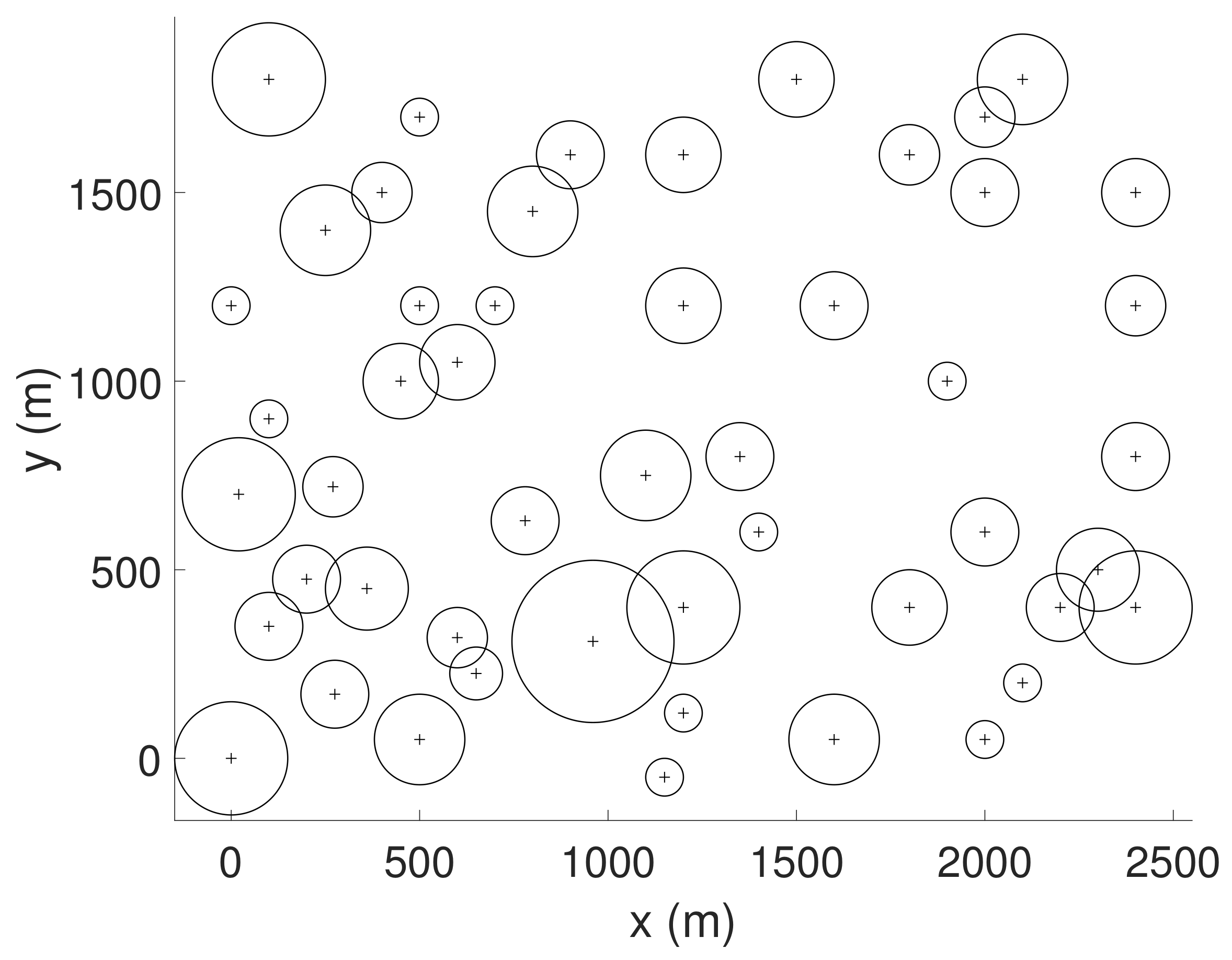
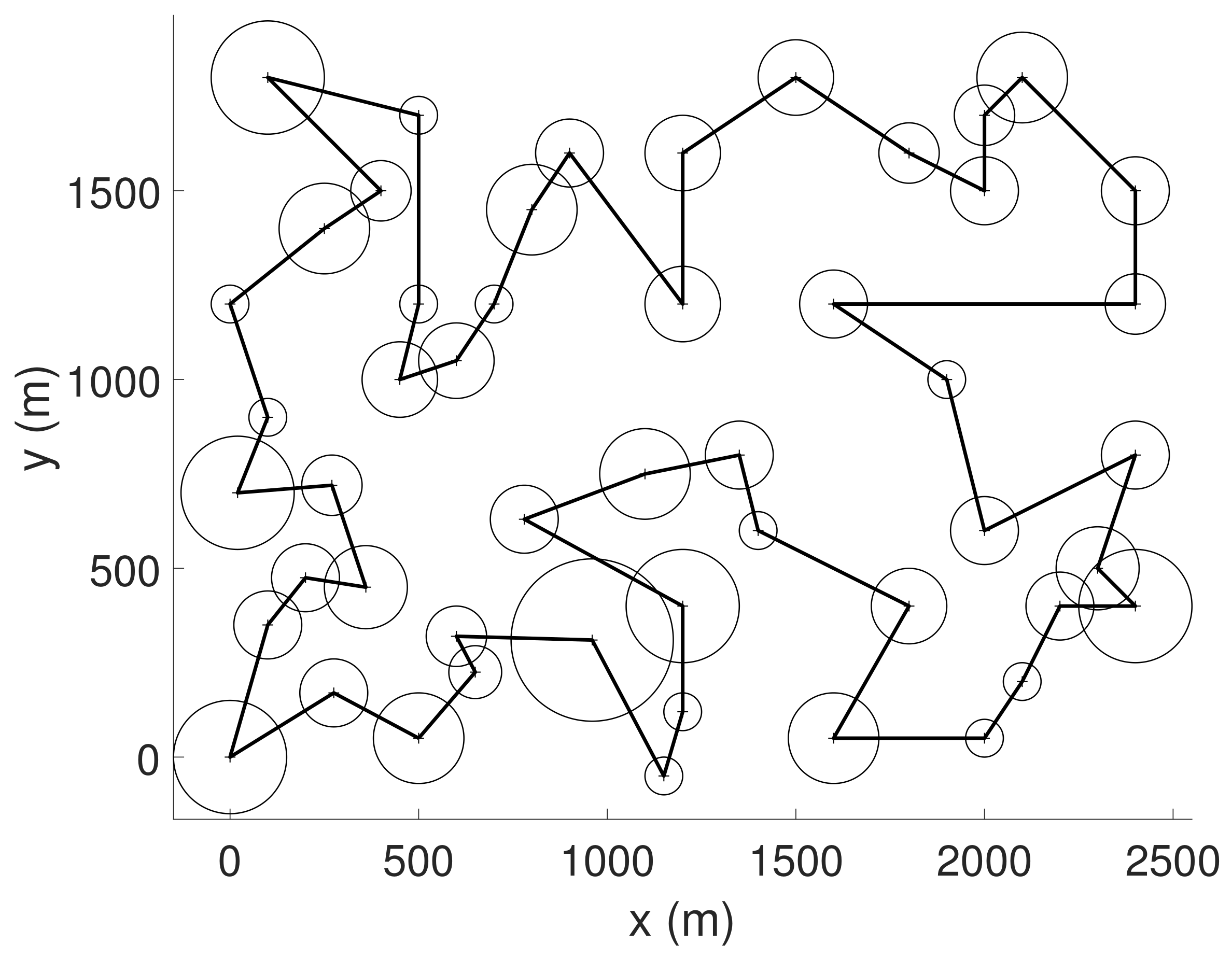
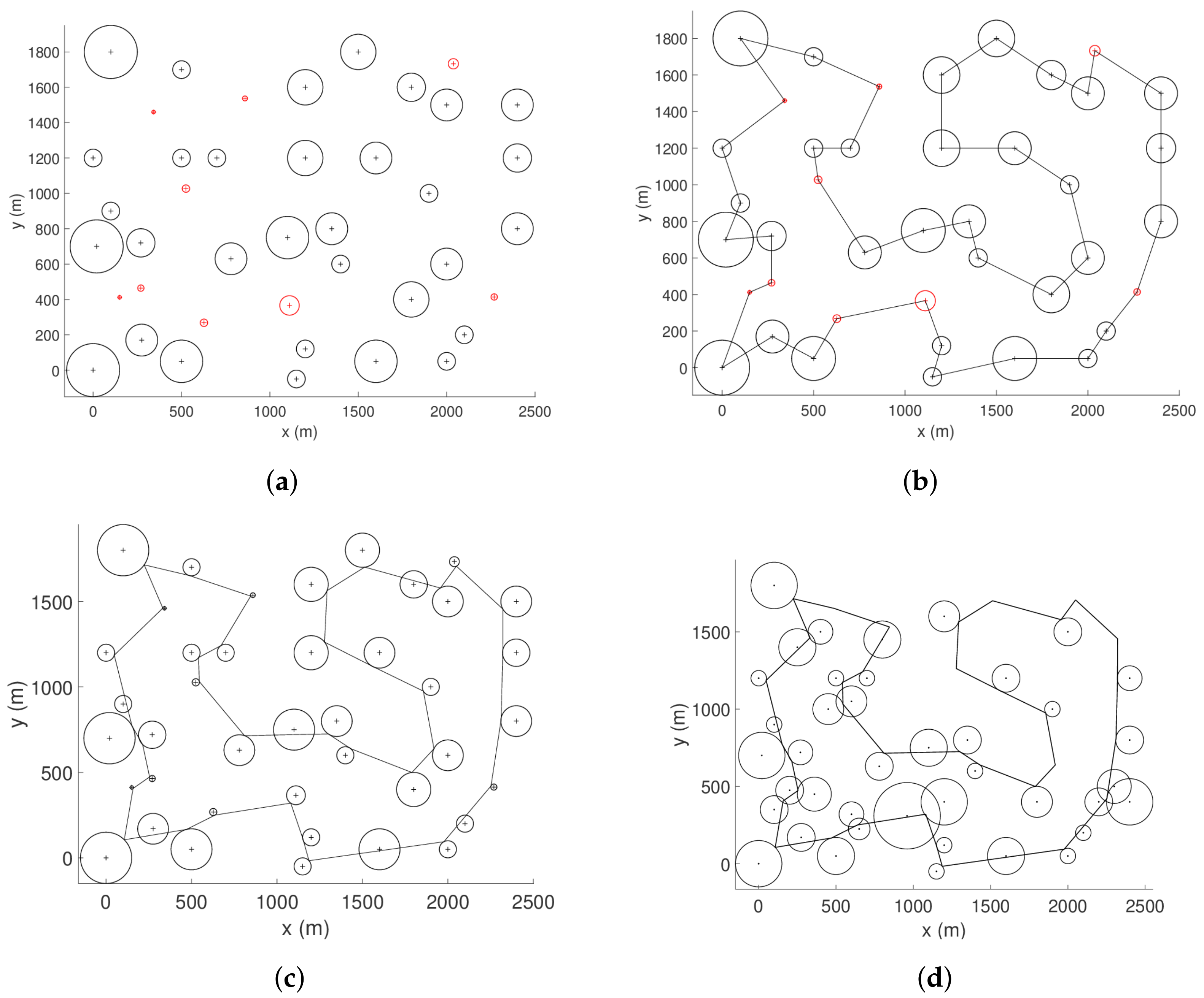
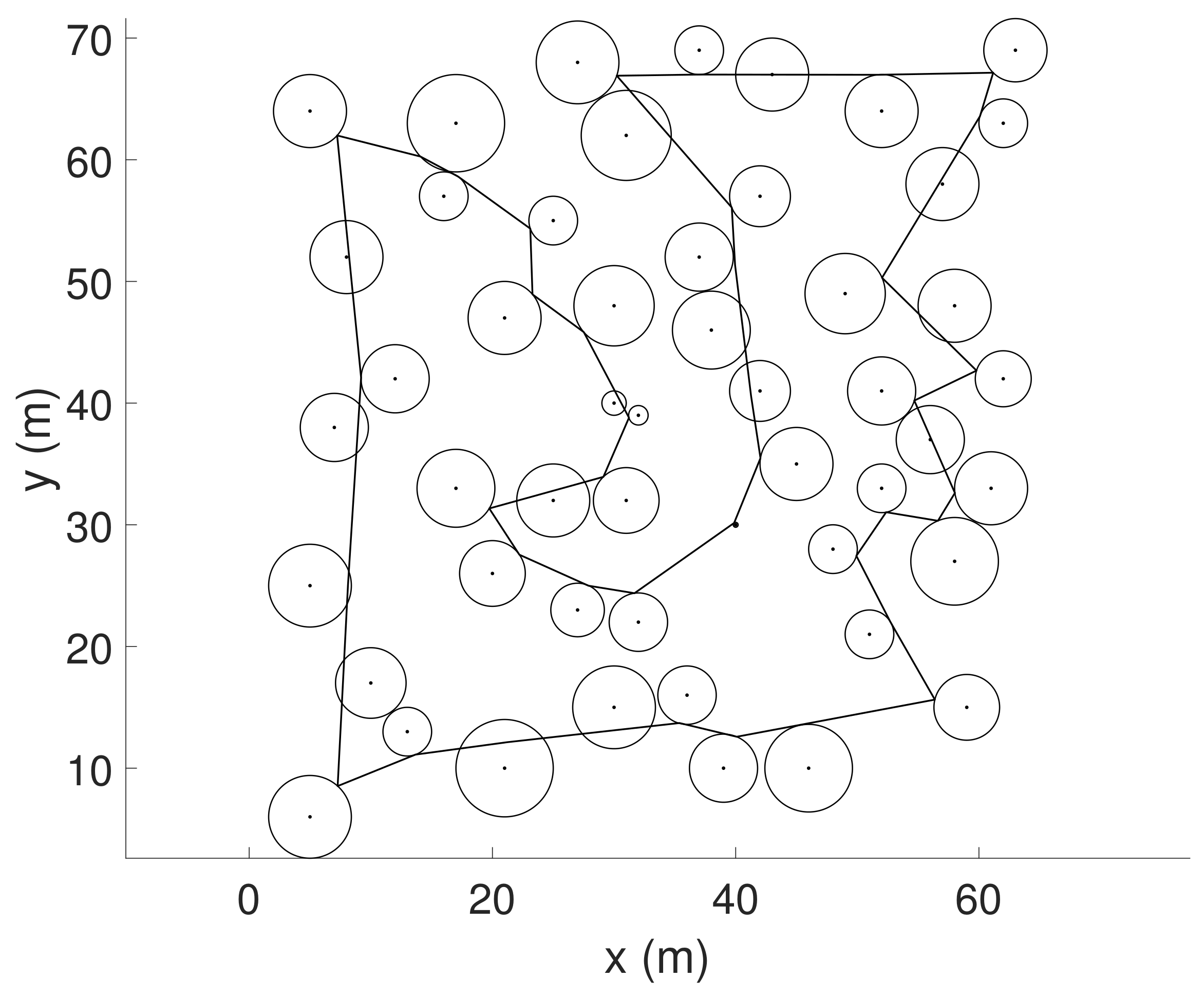
3.2. Test with 50 Nodes
4. Conclusions
5. Discussions and Future Work
5.1. Comparison with Other Works
5.2. Future Work
Author Contributions
Funding
Data Availability Statement
Acknowledgments
Conflicts of Interest
Abbreviations
| ATSP | Asymmetric Traveling Salesman Problem |
| CETSP | Close Enough Traveling Salesman Problem |
| CVRP | Capacited Vehicle Routing Problem |
| STSP | Symmetric Traveling Salesman Problem |
| TSP | Traveling Salesman Problem |
| TSPN | Traveling Salesman Problem with Neighborhoods |
| TSP-PC | Precedence Constrained Traveling Salesman Problem |
| UAV | Unmanned Aerial Vehicle |
| WUSN | Wireless Underground Sensor Network |
Appendix A

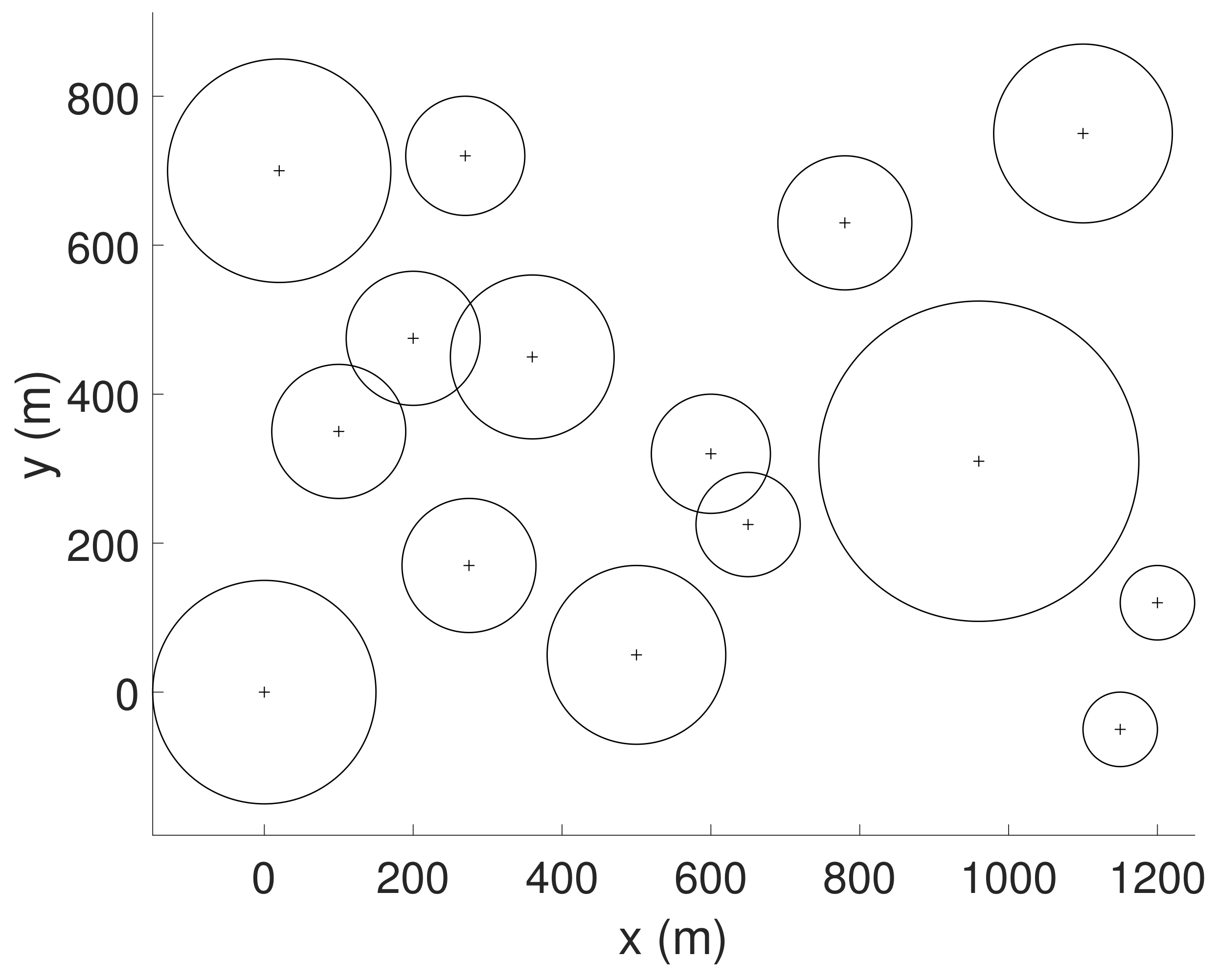
| n | Latitude (°) | Longitude (°) | x (m) | y (m) | Range (m) |
|---|---|---|---|---|---|
| 1 | 46.343386 | 3.434335 | 0 | 0 | 150 |
| 2 | 46.346520 | 3.435697 | 100 | 350 | 90 |
| 3 | 46.347632 | 3.437019 | 200 | 475 | 90 |
| 4 | 46.347387 | 3.439093 | 360 | 450 | 110 |
| 5 | 46.344879 | 3.437938 | 275 | 170 | 90 |
| 6 | 46.348953 | 3.444582 | 780 | 630 | 90 |
| 7 | 46.346051 | 3.446861 | 960 | 310 | 215 |
| 8 | 46.349827 | 3.437973 | 270 | 720 | 80 |
| 9 | 46.346187 | 3.442187 | 600 | 320 | 80 |
| 10 | 46.345326 | 3.442819 | 650 | 225 | 70 |
| 11 | 46.343771 | 3.440838 | 500 | 50 | 120 |
| 12 | 46.349679 | 3.434721 | 20 | 700 | 150 |
| 13 | 46.342789 | 3.449263 | 1150 | −50 | 50 |
| 14 | 46.344312 | 3.449944 | 1200 | 120 | 50 |
| 15 | 46.349992 | 3.448761 | 1100 | 750 | 120 |
| n | x (m) | y (m) | Radius (m) | n | x (m) | y (m) | Radius (m) |
|---|---|---|---|---|---|---|---|
| 1 | 0 | 0 | 150 | 26 | 2000 | 50 | 50 |
| 2 | 100 | 350 | 90 | 27 | 2100 | 200 | 50 |
| 3 | 200 | 475 | 90 | 28 | 2200 | 400 | 90 |
| 4 | 360 | 450 | 110 | 29 | 2300 | 500 | 110 |
| 5 | 275 | 170 | 90 | 30 | 2400 | 800 | 90 |
| 6 | 780 | 630 | 90 | 31 | 1600 | 50 | 120 |
| 7 | 960 | 310 | 215 | 32 | 1800 | 400 | 100 |
| 8 | 270 | 720 | 80 | 33 | 1900 | 1000 | 50 |
| 9 | 600 | 320 | 80 | 34 | 2400 | 1200 | 80 |
| 10 | 650 | 225 | 70 | 35 | 2400 | 400 | 150 |
| 11 | 500 | 50 | 120 | 36 | 250 | 1400 | 120 |
| 12 | 20 | 700 | 150 | 37 | 400 | 1500 | 80 |
| 13 | 1150 | −50 | 50 | 38 | 800 | 1450 | 120 |
| 14 | 1200 | 120 | 50 | 39 | 1200 | 1600 | 100 |
| 15 | 1100 | 750 | 120 | 40 | 2000 | 1500 | 90 |
| 16 | 1200 | 400 | 150 | 41 | 100 | 1800 | 150 |
| 17 | 1350 | 800 | 90 | 42 | 500 | 1700 | 50 |
| 18 | 1400 | 600 | 50 | 43 | 900 | 1600 | 90 |
| 19 | 0 | 1200 | 50 | 44 | 2000 | 1700 | 80 |
| 20 | 100 | 900 | 50 | 45 | 2100 | 1800 | 120 |
| 21 | 450 | 1000 | 100 | 46 | 1800 | 1600 | 80 |
| 22 | 500 | 1200 | 50 | 47 | 1500 | 1800 | 100 |
| 23 | 600 | 1050 | 100 | 48 | 2400 | 1500 | 90 |
| 24 | 700 | 1200 | 50 | 49 | 1200 | 1200 | 100 |
| 25 | 1600 | 1200 | 90 | 50 | 2000 | 600 | 90 |
| n | x (m) | y (m) | Radius (m) | n | x (m) | y (m) | Radius (m) |
|---|---|---|---|---|---|---|---|
| 1 | 37 | 52 | 2.8 | 27 | 30 | 48 | 3.3 |
| 2 | 49 | 49 | 3.3 | 28 | 43 | 67 | 3.0 |
| 3 | 52 | 64 | 3.0 | 29 | 58 | 48 | 3.0 |
| 4 | 20 | 26 | 2.7 | 30 | 58 | 27 | 3.6 |
| 5 | 40 | 30 | 0.2 | 31 | 37 | 69 | 2.0 |
| 6 | 21 | 47 | 3.0 | 32 | 38 | 46 | 3.2 |
| 7 | 17 | 63 | 4.0 | 33 | 46 | 10 | 3.6 |
| 8 | 31 | 62 | 3.7 | 34 | 61 | 33 | 3.0 |
| 9 | 52 | 33 | 2.0 | 35 | 62 | 63 | 2.0 |
| 10 | 51 | 21 | 2.0 | 36 | 63 | 69 | 2.6 |
| 11 | 42 | 41 | 2.5 | 37 | 32 | 22 | 2.4 |
| 12 | 31 | 32 | 2.7 | 38 | 45 | 35 | 3.0 |
| 13 | 5 | 25 | 3.4 | 39 | 59 | 15 | 2.5 |
| 14 | 12 | 42 | 2.8 | 40 | 5 | 6 | 3.4 |
| 15 | 36 | 16 | 2.4 | 41 | 10 | 17 | 2.9 |
| 16 | 52 | 41 | 2.8 | 42 | 21 | 10 | 4.0 |
| 17 | 27 | 23 | 2.2 | 43 | 5 | 64 | 3.0 |
| 18 | 17 | 33 | 3.2 | 44 | 30 | 15 | 3.4 |
| 19 | 13 | 13 | 2.0 | 45 | 39 | 10 | 2.8 |
| 20 | 57 | 58 | 3.0 | 46 | 32 | 39 | 0.8 |
| 21 | 62 | 42 | 2.3 | 47 | 25 | 32 | 3.0 |
| 22 | 42 | 57 | 2.5 | 48 | 25 | 55 | 2.0 |
| 23 | 16 | 57 | 2.0 | 49 | 48 | 28 | 2.0 |
| 24 | 8 | 52 | 3.0 | 50 | 56 | 37 | 2.8 |
| 25 | 7 | 38 | 2.8 | 51 | 30 | 40 | 1.0 |
| 26 | 27 | 68 | 3.4 |
References
- Grlj, C.G.; Krznar, N.; Pranjic, M. A Decade of UAV Docking Stations: A Brief Overview of Mobile and Fixed Landing Platforms. Drones 2022, 6, 7. [Google Scholar] [CrossRef]
- Aslan, M.F.; Durdu, A.; Sabanci, K.; Ropelewska, E.; Gultekin, S.S. A Comprehensive Survey of the Recent Studies with UAV for Precision Agriculture in Open Fields and Greenhouses. Appl. Sci. 2022, 12, 1047. [Google Scholar] [CrossRef]
- Srivastava, S.K.; Seng, K.P.; Ang, L.M.; Pachas, A.N.A.; Lewis, T. Drone-Based Environmental Monitoring and Image Processing Approaches for Resource Estimates of Private Native Forest. Sensors 2022, 22, 7872. [Google Scholar] [CrossRef] [PubMed]
- Nguyen, M.T.; Nguyen, C.V.; Do, H.T.; Hua, H.T.; Tran, T.A.; Nguyen, A.D.; Ala, G.; Viola, F. UAV-Assisted Data Collection in Wireless Sensor Networks: A Comprehensive Survey. Electronics 2021, 21, 2603. [Google Scholar] [CrossRef]
- Faiçal, B.S.; Pessin, G.; Filho, G.P.R.; Carvalho, C.P.L.F.; Gomes, P.H.; Ueyama, J. Fine-tuning of UAV control rules for spraying pesticides on crop fields: An approach for dynamic environments. Int. J. Artif. Intell. Tools 2016, 25, 1660003. [Google Scholar] [CrossRef]
- Ueyama, J.; Freitas, H.; Faiçal, B.S.; Filho, G.P.R.; Fini, P.; Pessin, G.; Gomes, P.H.; Villas, L.A. Exploiting the use of unmanned aerial vehicles to provide resilience in wireless sensor networks. IEEE Commun. Mag. 2014, 52, 81–87. [Google Scholar] [CrossRef]
- Cinar, A.; Korkmaz, S.; Kiran, M. A discrete tree-seed algorithm for solving symmetric traveling salesman problem. Eng. Sci. Technol. International J. 2020, 23, 879–890. [Google Scholar] [CrossRef]
- Tuani, A.; Keedwell, E.; Collett, M. Heterogenous adaptive ant colony optimization with 3-opt local search for the Travelling Salesman Problem. Appl. Soft Comput. 2020, 97, 106720. [Google Scholar] [CrossRef]
- Mersmann, O.; Bischl, B.; Bossek, J.; Trautmann, H.; Wagner, M.; Neumann, F. Local search and the Traveling Salesman Problem: A feature-based characterization of problem hardness. In Proceedings of the International Conference on Learning and Intelligent Optimization, Paris, France, 16–20 January 2012; Springer: Berlin/Heidelberg, Germany, 2012. [Google Scholar] [CrossRef]
- Katoch, S.; Chauhan, S.S.; Kumar, V. A review on genetic algorithm: Past, present, and future. Multimed. Tools Appl. 2021, 80, 8091–8126. [Google Scholar] [CrossRef]
- Qu, F.; Yu, W.; Xiao, K.; Liu, C.; Liu, W. Trajectory generation and optimization using the mutual learning and adaptive colony algorithm in uneven environments. Appl. Sci. 2022, 12, 4629. [Google Scholar] [CrossRef]
- Emambocus, B.A.S.; Jasser, M.B.; Hamzah, M.; Mustapha, A.; Amphawan, A. An enhanced swap sequence-based particle swarm optimization algorithm to Solve TSP. IEEE Access 2021, 9, 164820–164836. [Google Scholar] [CrossRef]
- Gambardella, L.M.; Dorigo, M. Solving symmetric and asymmetric TSPs by ant colonies. In Proceedings of the IEEE International Conference on Evolutionary Computation, Nagoya, Japan, 20–22 May 1996; pp. 622–627. [Google Scholar] [CrossRef]
- Sung, J.; Jeong, B. An adaptive evolutionary algorithm for traveling salesman problem with precedence constraints. Sci. World J. 2014, 2014, 313767. [Google Scholar] [CrossRef]
- Carwalo, T.; Thankappan, J.; Patil, V. Capacitated vehicle routing problem. In Proceedings of the 2nd International Conference on Communication Systems, Computing and IT Applications (CSCITA), Tokyo, Japan, 7–8 April 2017; pp. 17–21. [Google Scholar] [CrossRef]
- Berg, M.; Gudmundsson, J.; Katz, M. TSP with neighborhoods of varying size. In Proceedings of the 10th Annual European Symposium, Rome, Italy, 17–21 September 2002; pp. 187–199. [Google Scholar] [CrossRef]
- Sinha Roy, D.; Golden, B.; Wang, X.; Wasil, E. Estimating the tour length for the close enough traveling salesman problem. Algorithms 2021, 14, 123. [Google Scholar] [CrossRef]
- Semami, S.; Toulni, H.; Elbyed, A. The close enough traveling salesman problem with time window. Int. J. Circuits Syst. Signal Process. 2019, 13, 579–584. [Google Scholar]
- Huang, H.; Shi, J.; Wang, F.; Zhang, D. Theoretical and experimental studies on the signal propagation in soil for wireless underground sensor networks. Sensors 2020, 20, 2580. [Google Scholar] [CrossRef]
- Saeed, N.; Alouini, M.S.; Al-Naffouri, T. Towards the Internet of Underground Things: A systematic survey. IEEE Commun. Surv. Tutor. 2019, 21, 3443–3466. [Google Scholar] [CrossRef]
- Salam, A.; Raza, U. Current advances in Internet of Underground Things. In Signals in the Soil; Springer Nature Switzerland AG: Cham, Switzerland, 2020; Chapter 10; pp. 321–356. [Google Scholar] [CrossRef]
- Vuran, M.C.; Salam, A.; Wong, R.; Irmak, S. Internet of underground things: Sensing and communications on the field for precision agriculture. In Proceedings of the IEEE 4th World Forum on Internet of Things (WF-IoT), Singapore, 5–8 February 2018. [Google Scholar] [CrossRef]
- Silva, A.R.; Vuran, M.C. (CPS)2: Integration of center pivot systems with wireless underground sensor networks for autonomous precision agriculture. In Proceedings of the IEEE/ACM International Conference on Cyber-Physical Systems, Stockholm, Sweden, 13–15 April 2010; pp. 10–13. [Google Scholar] [CrossRef]
- Akyildiz, I.F.; Stuntebeck, E.P. Wireless underground sensor networks: Research challenges. Ad Hoc Netw. 2006, 4, 669–686. [Google Scholar] [CrossRef]
- Ferreira, C.B.M.; Peixoto, V.F.; de Brito, J.A.G.; de Monteiro, A.F.A.; de Assis, L.S.; Henriques, F.R. UnderApp: A system for remote monitoring of landslides based on wireless underground sensor networks. In Proceedings of the WTIC, Rio de Janeiro, Brazil, 1–2 April 2019. [Google Scholar]
- Moiroux-Arvis, L.; Cariou, C.; Chanet, J.P. Evaluation of LoRa technology in 433-MHz and 868-MHz for underground to aboveground data transmission. Comput. Electron. Agric. 2022, 194, 106770. [Google Scholar] [CrossRef]
- Fleischmann, B. A cutting plane procedure for the travelling salesman problem on road networks. Eur. J. Oper. Res. 1985, 21, 307–317. [Google Scholar] [CrossRef]
- Clausen, J. Branch and Bound Algorithms-Principles and Examples; Department of Computer Science, University of Copenhagen: Copenhagen, Denmark, 1999. [Google Scholar]
- Laporte, G. The traveling salesman problem: An overview of exact and approximate algorithms. Eur. J. Oper. Res. 1992, 59, 231–247. [Google Scholar] [CrossRef]
- Sanches, D.; Whitley, D.; Tinos, R. Improving an exact solver for the traveling salesman problem using partition crossover. In Proceedings of the Genetic and Evolutionary Computation Conference, Berlin, Germany, 15–19 July 2017; pp. 337–344. [Google Scholar] [CrossRef]
- Ozden, S.G.; Smith, A.E.; Gue, K.R. Solving large batches of traveling salesman problems with parallel and distributed computing. Comput. Oper. Res. 2017, 85, 87–96. [Google Scholar] [CrossRef]
- Hahsler, M.; Hornik, K. TSP—Infracstructure for the traveling salesperson problem. J. Stat. Softw. 2007, 23, 1–21. [Google Scholar] [CrossRef]
- Helsgaun, K. An Effective Implementation of K-Opt Moves for the Lin-Kernighan TSP Heuristic. Ph.D. Thesis, Roskilde University, Roskilde, Danmark, 2006. [Google Scholar]
- Helsgaun, K. An Extension of the Lin-Kernighan-Helsgaun TSP solver for Constrained Traveling Salesman and Vehicle Routing Problems; Roskilde University: Roskilde, Denmark, 2017. [Google Scholar] [CrossRef]
- Razali, N.M.; Geraghty, J. Genetic algorithm performance with different selection strategies in solving TSP. In Proceedings of the World Congress on Engineering; International Association of Engineers: Hong Kong, China, 2011; Volume 2. [Google Scholar]
- Yang, J.; Shi, X.; Marchese, M.; Liang, Y. An ant colony optimization method for generalized TSP problem. Prog. Nat. Sci. 2008, 18, 1417–1422. [Google Scholar] [CrossRef]
- Gulczynski, D.; Heath, J.; Price, C. Close enough traveling salesman problem: A discussion of several heuristics. Perspect. Oper. Res. 2006, 36, 271–283. [Google Scholar]
- Dong, J.; Yang, N.; Chen, M. Heuristic approaches for a TSP variant: The automatic meter reading shortest tour problem. In Extending the Horizons: Advances in Computing, Optimization, and Decision Technologies; Springer: New York, NY, USA, 2007. [Google Scholar]
- Mennell, W.; Golden, B.; Wasil, E. A steiner-zone heuristic for solving the close-enough traveling salesman problem. In Proceedings of the 12th INFORMS Computing Society Conference, Homeland Defense, Monterey, CA, USA, 9–11 January 2011. [Google Scholar]
- Coutinho, W.P.; Nascimento, R.Q.; Pessoa, A.A.; Subramanian, A. A Branch-and-Bound algorithm for the Close-Enough Traveling Salesman Problem. Informs J. Comput. 2016, 28, 752–765. [Google Scholar] [CrossRef]
- Elbassioni, K.; Fishkin, A.; Mustafa, N.; Sitters, R. Approximation Algorithms for Euclidian Group TSP. In Proceedings of the International Colloquium on Automata, Languages, and Programming, Lisbon, Portugal, 11–15 July 2005; Springer: Berlin/Heidelberg, Germany, 2005; pp. 1115–1126. [Google Scholar] [CrossRef]
- Carrabs, F.; Cerrone, C.; Cerulli, R.; Gaudioso, M. A novel discretization scheme for the Close Enough Traveling Salesman Problem. Comput. Oper. Res. 2007, 78, 163–171. [Google Scholar] [CrossRef]
- Yuan, B.; Orlowska, M.; Sadiq, S. On the optimal robot routing problem in wireless sensor networks. IEEE Trans. Knowl. Data Eng. 2007, 19, 1252–1261. [Google Scholar] [CrossRef]


Disclaimer/Publisher’s Note: The statements, opinions and data contained in all publications are solely those of the individual author(s) and contributor(s) and not of MDPI and/or the editor(s). MDPI and/or the editor(s) disclaim responsibility for any injury to people or property resulting from any ideas, methods, instructions or products referred to in the content. |
© 2023 by the authors. Licensee MDPI, Basel, Switzerland. This article is an open access article distributed under the terms and conditions of the Creative Commons Attribution (CC BY) license (https://creativecommons.org/licenses/by/4.0/).
Share and Cite
Cariou, C.; Moiroux-Arvis, L.; Pinet, F.; Chanet, J.-P. Evolutionary Algorithm with Geometrical Heuristics for Solving the Close Enough Traveling Salesman Problem: Application to the Trajectory Planning of an Unmanned Aerial Vehicle. Algorithms 2023, 16, 44. https://doi.org/10.3390/a16010044
Cariou C, Moiroux-Arvis L, Pinet F, Chanet J-P. Evolutionary Algorithm with Geometrical Heuristics for Solving the Close Enough Traveling Salesman Problem: Application to the Trajectory Planning of an Unmanned Aerial Vehicle. Algorithms. 2023; 16(1):44. https://doi.org/10.3390/a16010044
Chicago/Turabian StyleCariou, Christophe, Laure Moiroux-Arvis, François Pinet, and Jean-Pierre Chanet. 2023. "Evolutionary Algorithm with Geometrical Heuristics for Solving the Close Enough Traveling Salesman Problem: Application to the Trajectory Planning of an Unmanned Aerial Vehicle" Algorithms 16, no. 1: 44. https://doi.org/10.3390/a16010044
APA StyleCariou, C., Moiroux-Arvis, L., Pinet, F., & Chanet, J.-P. (2023). Evolutionary Algorithm with Geometrical Heuristics for Solving the Close Enough Traveling Salesman Problem: Application to the Trajectory Planning of an Unmanned Aerial Vehicle. Algorithms, 16(1), 44. https://doi.org/10.3390/a16010044