Deep Reinforcement Learning-Based Dynamic Pricing for Parking Solutions

Abstract

The growth in the number of automobiles in metropolitan areas has drawn attention to the need for more efficient carpark control in public spaces such as healthcare, retail stores, and office blocks. In this research, dynamic pricing is integrated with real-time parking data to optimise parking utilisation and reduce traffic jams. Dynamic pricing is the practice of changing the price of a product or service in response to market trends. This approach has the potential to manage car traffic in the parking space during peak and off-peak hours. The dynamic pricing method can set the parking fee at a greater price during peak hours and a lower rate during off-peak times. A method called deep reinforcement learning-based dynamic pricing (DRL-DP) is proposed in this paper. Dynamic pricing is separated into episodes and shifted back and forth on an hourly basis. Parking utilisation rates and profits are viewed as incentives for pricing control. The simulation output illustrates that the proposed solution is credible and effective under circumstances where the parking market around the parking area is competitive among each parking provider.

1. Introduction

A major problem in many metropolitan areas, particularly in major cities such as London, Hong Kong and Kuala Lumpur, is the dramatic rise of private automobiles. The growing number of automobiles has detrimental effects on both the local population and the surroundings. The growing number of automobiles increases the need for parking spaces. A 2017 poll conducted by New Strait Times found that the average time spent seeking parking in certain urban areas is roughly 25 min per day. The cars continue to circle the location, wasting time looking for an open parking lot. This increases fuel consumption and emissions of carbon dioxide which devastate the climate and generate the greenhouse effect. The greater the time driver spent on driving, the greater the traffic jam in that region. This starts a domino effect that aggravates other drivers and causes more delays.

Numerous academics have attempted to address the issues of traffic congestion and the enormous demand for parking lots after realising the difficulties brought on by the growth in the number of automobiles. Parking information, such as the availability of free parking spaces, can be received in real time using technologies such as sensors (loop or ultrasonic sensor), tickets or e-payment systems. This offers a chance to develop a smart parking system with dynamic pricing. To maximise the income and simultaneously improve parking space utilisation, the parking vendor can provide adjustable price regulation depending on various periods of time by adopting dynamic pricing.

In this research, a deep reinforcement learning-based dynamic pricing (DRL-DP) model is proposed to manage parking prices depending on vehicle volume and parking occupancy rate. Because it does not require raw labelled data in environment modelling, reinforcement learning (RL) is recommended. RL makes it possible to make decisions sequentially and offers a complete series of wise choices throughout the experiments. The dynamic pricing model keeps track of various price plans and how they are used in various contexts to reduce traffic congestion and increase profits for parking vendors. The dynamic pricing model distributes vehicle flows and predicts vehicle volume and traffic congestion. By suppressing drivers’ visits to a certain region during peak hours at specified intervals of the day, the vehicle flows are distributed to non-peak hours to boost the parking utilisation rate and decrease traffic jams. This is accomplished by controlling prices through price reductions such as parking payment cash back. In order to improve the returned incentive in the following episode, the deep learning agent will learn from the sequential choice of dynamic pricing.

The remainder of this article is structured as follows. Section 2 covers related research on topics including dynamic pricing and smart parking. The proposed approach is described in Section 3. The experiment’s findings are presented in Section 4. The final section, Section 5, discusses further developments.

2. Literature Review

2.1. Dynamic Pricing

Because e-commerce is now a common choice for business models, dynamic pricing has been a pricing technique that has a significant impact on our society. The Internet allows any trade-off, saves many physical costs and has facilitated simple market entrance. Due to the availability of giant data that make user behaviour transparent, many academics are now concentrating on dynamic pricing in e-commerce.

Four pricing techniques for e-commerce were given by Karpowicz and Szajowski [1]: (1) time-based pricing; (2) market segmentation and restricted rations; (3) dynamic marketing; (4) the combined usage of the aforementioned three kinds. On the other hand, Chen and Wang [2] presented a data mining-based dynamic pricing model for e-commerce. The data layer, analytical layer and decision layer were the three bottom-up layers that made up the model.

The best pricing strategy for an agent in a multi-agent scenario is influenced by the strategies used by the other agents [3]. Han et al. [3] suggested a multi-agent reinforcement learning system that incorporates both the opponents’ inferential intentions and their observed objective behaviours. A novel continuous time model with price and time-sensitive demand was presented by Pan et al. [4] to take into consideration of dynamic pricing usage, order cancellation ratios and various quality of service (QoS) levels in online networks.

Reinforcement learning (RL) was suggested as a method by Chinthalapati et al. to examine pricing dynamics in a digital commercial market [5]. The suggested strategy involved two vendors in competition, price and lead time-sensitive customers. They took into account the no-information scenario and the partial information situation as two illustrative examples. In order to establish dynamic pricing on the internet, Ujjwal et al. [6] presented a bargaining agent that made use of a genetic algorithm. Because the mutually agreed deal price is greater than the seller’s reserved price but lesser than the buyer’s reserved price, online bargaining benefits both the seller and the buyer.

The authors in [7] suggested Pareto-efficient and subgame-perfect equilibrium and provided a bounded regret over an infinite horizon. They defined regret as the anticipated cumulative profit loss in comparison to the ideal situation with a known demand model. However, they presupposed that all vendors faced equal marginal costs when considering an oligopoly with dynamic pricing in the face of demand uncertainty.

Another research in [8] examined companies’ pricing policies in the presence of ambiguous demand. Reference prices and the cost of competition, per the study, were the two variables that impacted demand dynamics. Results from simulations showed that companies might reduce the volatility of their pricing path if they collected and analysed customer data and competition since doing so allowed them more control than ever before over uncertainty.

In the scenario that supply exceeds demand or vice versa, Wang [9] suggested a dynamic pricing mechanism for the merchant. The study determined the best dynamic pricing techniques and stated the equilibrium conditions for those strategies.

“Compared to the myopic, strategic consumers may have stronger incentive to delay the purchase once they perceive that a signifcant cost reduction will result in a markdown” [10]. Liu and Guan examined the cost-cutting impact of dynamic pricing on a market with both myopic and strategic customers. Their study showed that consumers tend to delay the purchase when a significant cost-cutting is available, especially for strategic customers.

Recently, dynamic pricing research mainly focuses on the financial aspect. Mathematical models are adopted to calculate dynamic pricing based on different game theories applied in different circumstances. Some of the studies have yet to combine dynamic pricing with transdisciplinary research such as artificial intelligence (AI). In fact, there is some dynamic pricing research that utilises AI components, but they only focus on e-commerce online platforms such as TaoBao and Shoppee which analyse user behaviour on their platforms.

2.2. Smart Parking Solutions

In order to successfully deploy on a broad scale, parking solutions incorporate knowledge from several fields. Recent developments, such as the 5G network, also make real-time machine-to-machine (M2M) communication feasible. There are a few review articles that offer a useful perspective on the most current smart solutions utilising various technologies. According to the objectives of the many study domains, intelligent parking systems are divided into three macro-themes in [11]: data gathering, system implementation and service diffusion.

An intelligent resource allocation, reservation and pricing framework was presented in the paper published in [12] as the foundation of an intelligent parking solution. The solution provided drivers with assured parking reservations at the lowest feasible cost and seeking duration while also providing parking managers with the maximum income and parking usage rate. A crowdsourcing method called ParkForU was presented by Mitsopoulou and Kalogeraki [13] to locate the available and most practical parking alternatives for users in a smart city. It was a car park matching and pricing regulator technique that let users enter their destination as well as a list of preferences for price and distance (from the car park to their desired location), as well as the total amount of matches they wanted to see.

Nugraha and Tanamas suggested a dynamic allocation approach to reserve car parks using Internet applications in [14]. Finding the empty parking lot and making the booking for the car owner removed the requirement to look through the whole parking zone. To keep the parking lot’s utilisation level, they employed an event-driven schema allocation when a car pulled up to the gate.

In [15], the authors suggested a carpooling model using two matching algorithms that followed the single and dual side matching approach to give additional alternatives on grab time and cost, allowing travellers to select the car that best suits their preferences. The default approach for carpooling matching techniques entered a request for a ride into a kinetic tree and returned all feasible matches of grab time and cost that did not prevail over one another.

Jioudi et al. [16] presented a dynamic pricing scheme that modifies costs proportionately to the arrival time upon every carparks and, as a result, lessens congestion and gets rid of drivers’ preferences for particular carparks. They used the discrete batch arrival process (D-BMAP) to assess the parking time in close to real-world circumstances. According to their parking time, the drivers that arrived in accordance with D-BMAP were chosen for service in random order (ROS).

In [17], the authors sought to enhance the rotation of prime locations and establish a usage-based carpark allocation through the use of a suitable reward, which is the same as using tactical pricing to reduce parking average waiting time and enhance traffic situation in the intended area. Decreasing the number of long-term parking spaces and taking appropriate steps to allow short-term parking is essential for improving the use of insufficient parking spaces in demanded regions.

Two prediction models were presented by the authors in [18] for the qualitative and quantitative enhancement of parking availability data. The term “quality problem” refers to the network latency between parking sensors and the data server as well as the preset update interval. The term “quantity problem” refers to unsupervised, non-smart parking lots. In order to increase quality, a future availability forecasting model was created by studying the trend of parking and variations in occupancy rate using past data. By supposing the prediction of target’s occupancy rate might be predicted using occupancy rate data from neighbouring smart parking for quantity enhancement, they also presented an availability forecasting method for non-smart parking spaces that were not fitted with sensors.

In [19], the authors presented a macroscopic parking pricing and decision model for responsive parking pricing. They considered the value of time, parking fee and search time cost of a driver to get the vacant parking and analysed the short-term influence on the traffic.

A dynamic pricing model was presented by [20] for parking reservations to maximise the parking revenue. The dynamic pricing model was formulated as a stochastic dynamic programming problem in the paper. The efficacy of the parking schema is provided in the numerical experiments to increase parking profit and decrease drivers’ circling expenses.

The aforementioned recent study concentrates on reservations or pricing regulation using real-time algorithms and providing users with results of smart parking systems. For instance, ParkForU [13] uses parking matching and price regulator algorithm, notifying parking vendors after a driver’s decision and adjusting their price adaptively to impress the driver, while iParker [12] utilises real-time booking requests with share time booking to discover the vacant and most adequate parking selection for the user. A reservation-based parking system [14] uses the driver’s estimated time of arrival to allocate open spaces and dynamically redistribute spaces when a specific automobile arrives without a booking.

Jioudi et al. [16] utilised a dynamic pricing approach that adjusts prices in accordance with arrival time. By permitting them to park in the most desirable zones, Jioudi et al. [17] exploited area zonification to promote short and mid-term parking stays. K. N. and Kim Koshizuka [18] used two forecasting methods for the qualitative and quantitative augmentation of parking availability data. In order to propose a suitable discount scheme to optimise parking occupancy utilisation and reduce traffic congestion, we intended to utilise dynamic pricing and reinforcement learning in this work to estimate future arrival rates. The simulation may be created for many scenarios using the suggested system, taking into account the number of parking operators, their price structures and the volume of traffic in the parking space. This improved the proposed method’s dependability.

3. Proposed Method

This study presents a deep reinforcement learning-based dynamic pricing (DRL-DP) model for training the dynamic pricing mechanism using a reinforcement learning approach. The suggested model functions as a market environment for the parking sector. A parking vendor and the other competitors (the other parking vendors) in this setting play the role of the player. The number of cars which park in the player’s parking space and the money made from parking are the rewards.

We concentrate on smoothing the regression distribution model of the past parking utilisation rate by raising the utilisation rate during non-peak hours, in contrast to prior smart parking research that focuses on reservations for drivers and pricing regulation by parking providers.

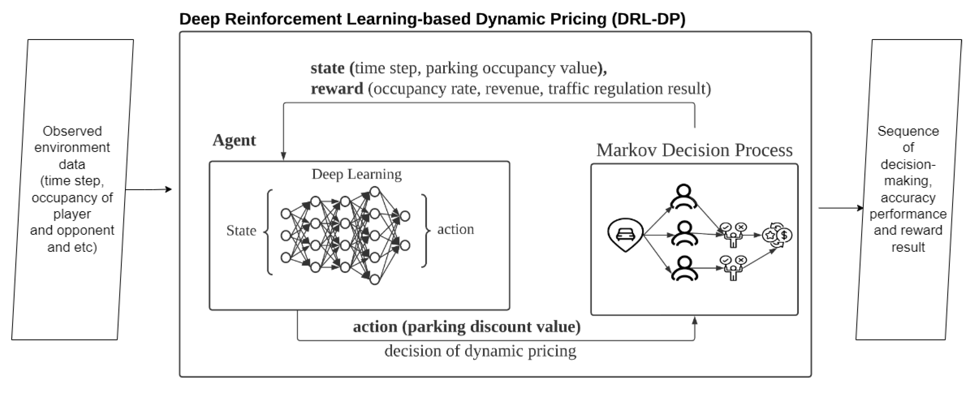
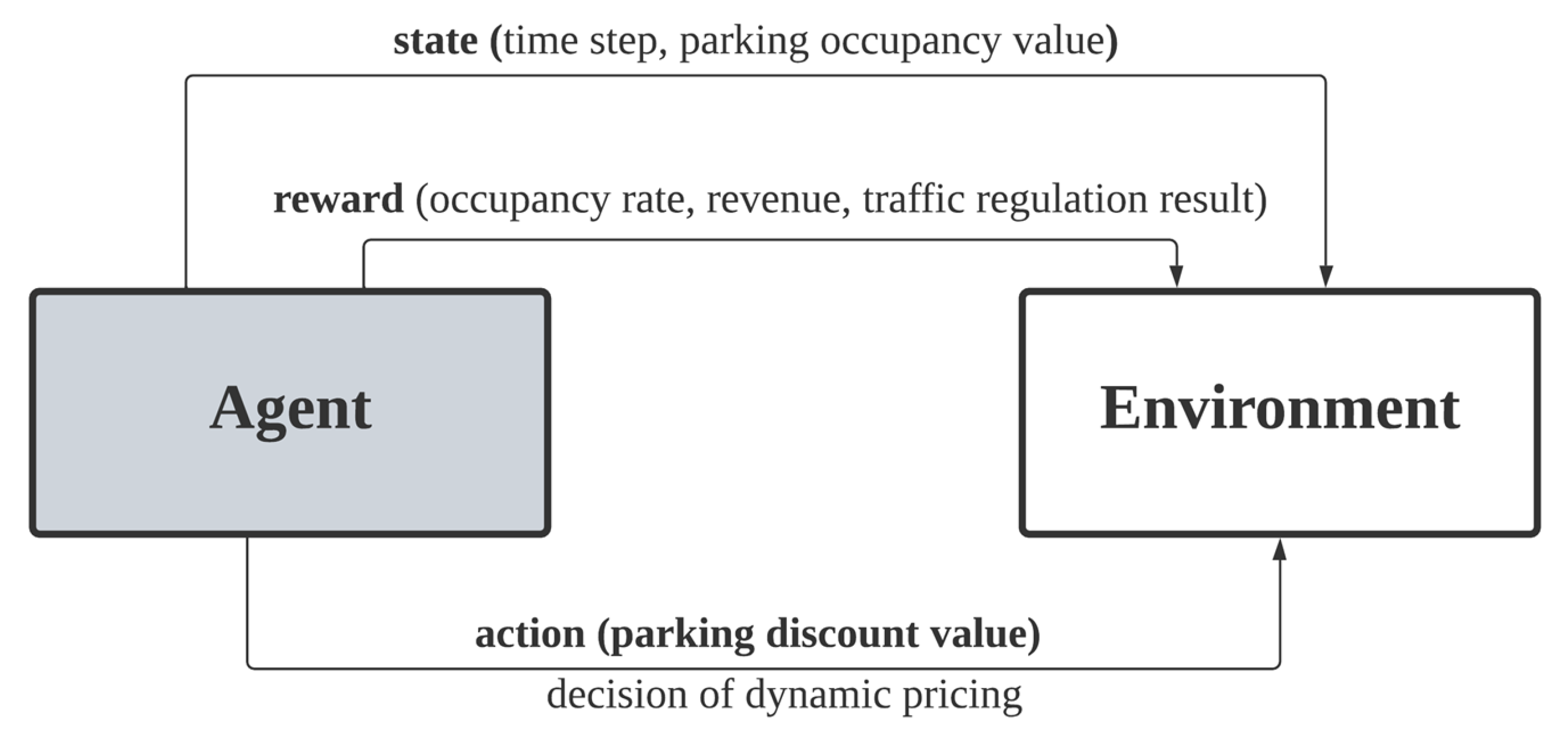
In reinforcing learning, the deep learning agent learns to achieve a higher reward using the returned reward from the environment. In the proposed environment, the state represents the time step and parking occupancy ratio of the player and opponent, the action represents the discount value of dynamic pricing, while rewards constitute the vehicle arrival rate, parking revenue and vehicle flow regulation result. The environment is a sequential decision-making process to decide whether a parking lot will be taken in the dynamic pricing problem. The environment is formulated using the Markov decision process (MDP) to achieve rewards for the player with each action taken. MDP receives the discount action of the player and decision making of the drivers and returns the decision of the drivers as a reward to the environment. In the parking environment simulation, MDP demonstrates the drivers’ decisions based on prices regulated by the parking vendors. Thus, MDP simulates the drivers’ decision based on the forecasted vehicle flow in every time step to obtain the reward. Figure 1 shows the block diagram of the proposed method, which is comprised of deep learning and Markov decision processes.

In the proposed method, environment data such as time-step, pricing scheme and occupancy of the player and opponent are input to DRL-DP. DRL-DP simulates the parking environment using the input data. After that, DRL-DP outputs the sequence of decision-making, accuracy performance and reward result from the simulation. The environment simulator utilises the vehicle flow prediction from SARIMAX as the vehicle flow around the parking area. Multiple modules are constructed to assist the parking market simulation such as a pricing engine and grid system. The details of each module are presented in Section 3.2.2.

3.1. Datasets

3.1.1. Data Collection

In this study, the in- and outflows of the vehicle at parking premises are collected. An IoT device is attached to the barrier gate and the number of vehicles coming in and out from the parking premise is recorded based on the movement of the barrier gate. The data received in the loop sensor in a real-world road network may be affected by noise. Thus, the vehicle arrival rate of certain parking areas is collected using a sensor in the barrier gate. Once the barrier gate rises for incoming or outgoing vehicles, the IoT will record and trace vehicle plates using a camera with vehicle plate recognition. With the data collection using IoT in the barrier gate, the in and out records with vehicle stay time can be collected and analysed.

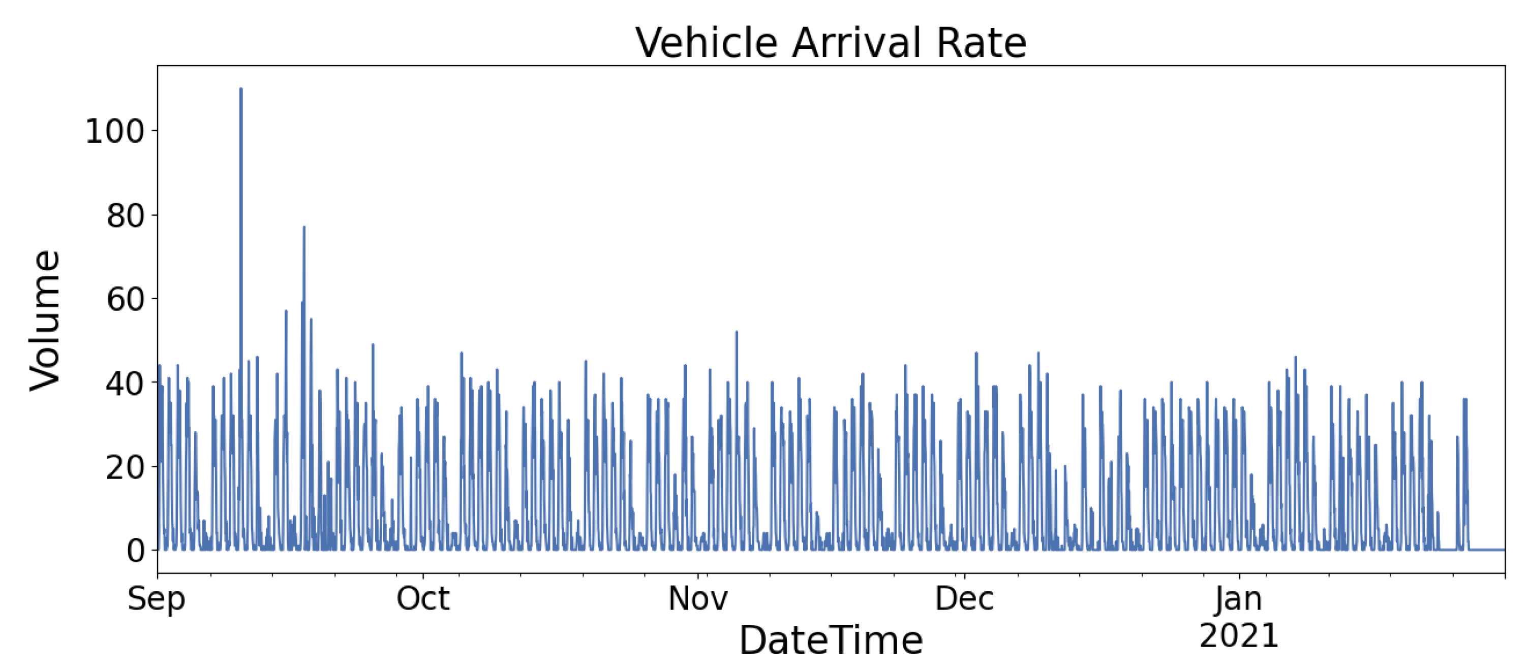
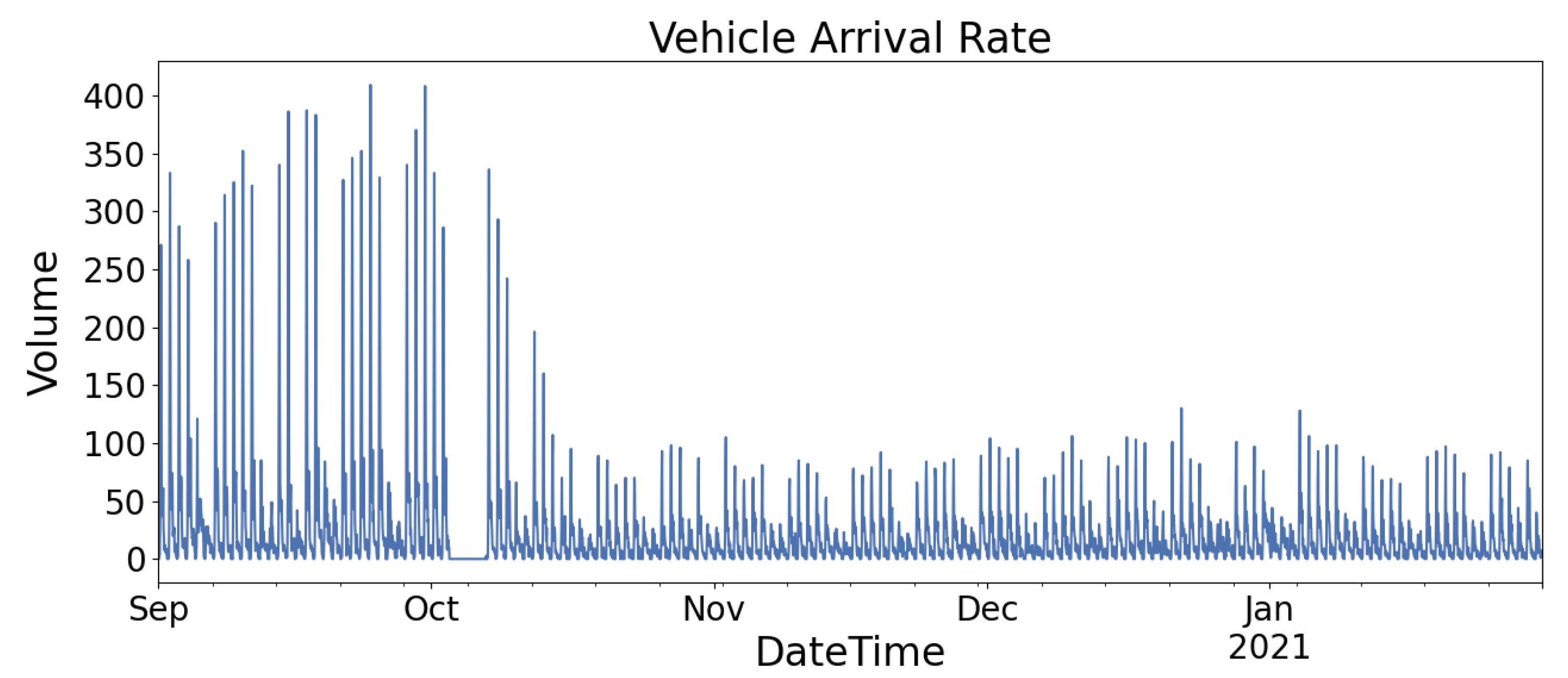
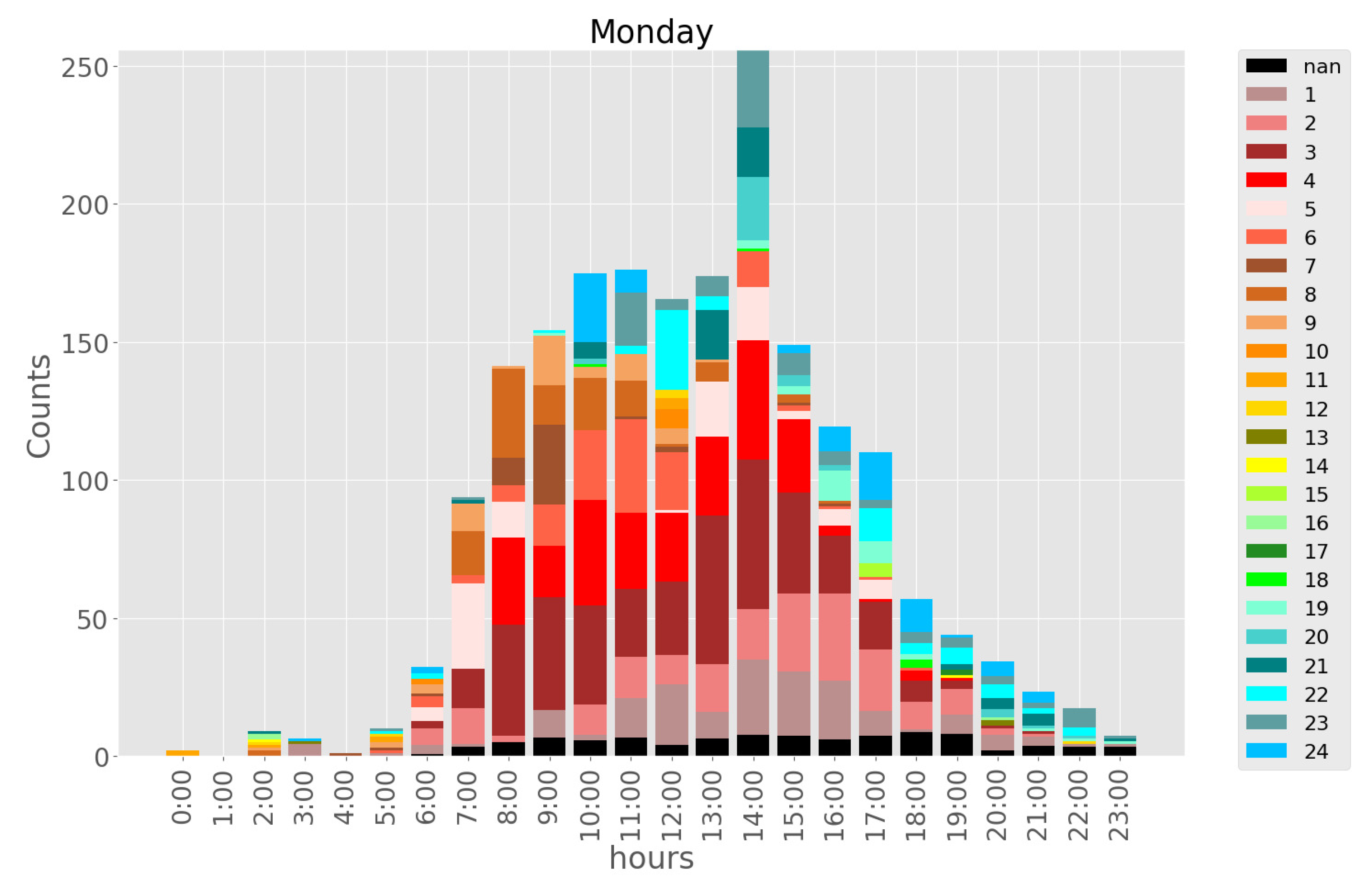
In this study, the parking data are collected from two locations, denoted as Location A and Location B, for a period of about six months. The two locations are parking areas in busy commercial areas in Kuala Lumpur, Malaysia. Due to privacy and confidentiality issues, the location names could not be disclosed. Figure 2 and Figure 3 show the graph of the vehicle arrival rate of Location A and Location B, respectively. Both figures show that Location A and Location B demonstrate similar vehicle flow patterns, higher arrival rates during the weekday (Monday to Friday) and lower arrival rates during the weekend (Saturday and Sunday). Location A has a parking capacity of 165 while Location B has a parking capacity of 950. Thus, they have different peak vehicle arrival rates because of their capacities.

3.1.2. Data Extraction

In the proposed method, environment simulation is the most conclusive component because it influences the accuracy and reliable interactive feedback between the agent action and the environment. Thus, valuable environment parameters such as parking capacity, pricing policy and vehicle arrival rate as the controllable variables are important to simulate a reliable and robust real-world model. From real-time parking occupancy, the vehicle arrival rates for each hour are extracted and analysed. Different parking areas have different types of visitors, such as short-term (intermittent) visitors and long-term visitors. From the vehicle stay time, the visitor type of that parking area can be identified because the visitor type will influence the pricing policy and discount scheme used in the simulation model.

3.1.3. Parking Occupancy Data (Arrival In- and Outflow)

The parking occupancy data are collected from Location A and Location B from September 2020 to Jan 2021. The parking occupancy data represents the in and out events in the parking space. Performing dynamic pricing in the parking industry will result in affecting the vehicle arrival rate because it will affect the driver’s willingness to park in different parking areas. Thus, forecasting future vehicle arrival rates is an important part of the proposed solution to increase robustness in the face of different situations affecting the vehicle arrival rate. SARIMAX (Seasonal Auto-Regressive Integrated Moving Average with eXogenous factors) [21] is used to forecast future in and out arrival, which will be used in the RL simulations. SARIMAX is an updated version of ARIMA which includes an autoregressive integrated moving average, while SARIMAX includes seasonal affect and eXogenous factors, so it can deal with datasets that have seasonal cycles.

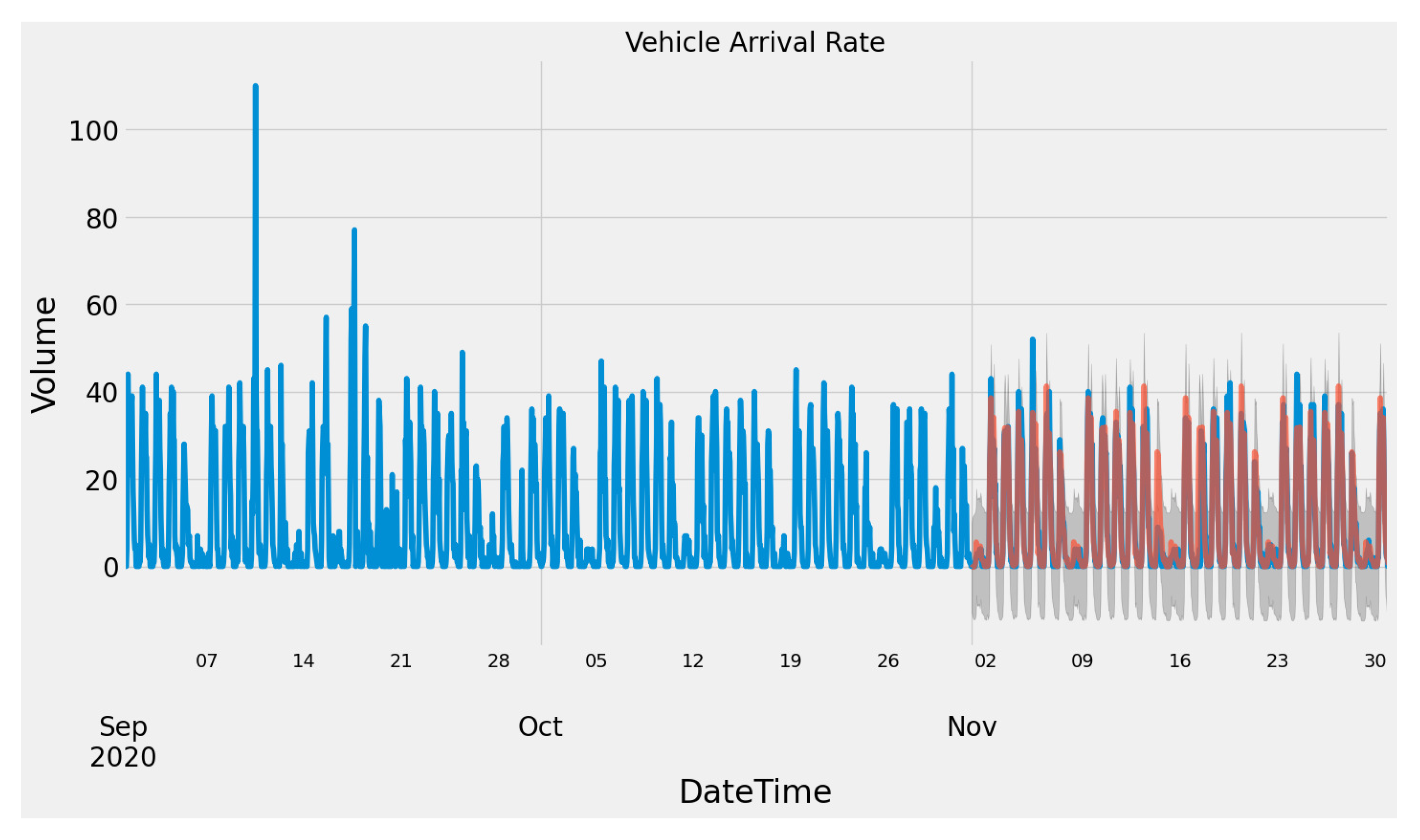
Figure 4 and Figure 5 show the arrival in and out of the sample parking area. In Figure 5, blue color line represents the observed vehicle arrival rate, orange color represents the one-step ahead forecast vehicle arrival rate, the shadowed region represents the confidence interval of predicted arrival rate. A repeating pattern can be observed from the pattern of arrival flow. Thus, the SARIMAX model can forecast future vehicle arrival with high accuracy using three months of training data (Figure 3). The RL simulation will use the forecasted arrival flow for both the player and the opponent.

3.1.4. Vehicle Stay Time

The vehicle stay times are extracted from the parking occupancy data from Section 3.1.1. Vehicle stay time analysis can be used to predict the vehicle stay time in RL simulation and calculate the parking fee of each parking vendor with the aid of the driver to make a decision. Figure 6 shows the vehicle stay time analysis graph of the sample parking area. The vehicle stay time was arbitrary, but the vehicle mostly stays within one to five hours.

3.2. Deep Reinforcement Learning-Based Dynamic Pricing (DRP-DP)

In this section, the decision-making components of the proposed DRL-DP method are defined and discussed. The main components in RL are the agent and environment. The agent performs actions while the environment returns the state (observation) and reward (incentive mechanism where the benefit is obtained by the player through the action).

In DRL-DP, the deep learning agent acts as an agent to maximise the reward from the environment. The deep learning agent uses the state (observation of the environment, including time step and occupancy of player and opponent) as inputs and outputs the action (discount value taken by the player). The actions are retrieved by the environment and modelled by the Markov decision process (MDP). In a parking environment, the MDP’s state is initiated with the action retrieved from the player. Then, MDP initialises the driver with the numbers of vehicle flow in the current time step. Each driver undergoes decision making to decide whether to park at the parking lot. The reward (including occupancy rate, accumulated revenue and comparison of vehicle arrival with targeted arrival after vehicle flow regulation) in the current time step is obtained as the result of MDP. The state and reward are forwarded to the deep learning agent to learn and maximise the revenue in the next episode.

3.2.1. Notation and Assumption

In this study, the players and opponents refer to the parking vendors, respectively. They compete with each other to get a higher occupancy rate and revenue. Each parking vendor is assumed to have at least one pricing scheme for their parking fee. The highest and lowest parking costs for the driver are included in the pricing policy. At the beginning of the simulation, each of the players and the competitors shall decide on the parking lot’s overall capacity as well as the maximum and lowest parking rates. The following presumptions are made on how vehicle flows relate to one another:

• A weekly iteration with a global reward reset on every episode that lasts seven days is referred to as an episode.
• Maximising parking utilisation, maximising driver contentment and maximising business income are issues that parking operators must take into account.
• Parking vendors with pricing scheme: arrival-time-dependent pricing (ATP)—the driver pays the parking fee by calculating the arrival time of the driver’s vehicle without considering the parking interval (flat rate); progressive pricing—the driver pays the parking fee by calculating the parking interval of the driver without considering the arrival time, etc.
• The pricing engine calculates the parking fee based on the arrival time and the vehicle stay time by referring to the pricing policy of the parking vendor.
• The parking market demands are predicted by calculating past vehicle flow (entry and exit) as demand and supply rate.
• The episode rewards are calculated from occupancy and revenue obtained at each hour and normalised at each period section to yield a global revenue.

3.2.2. Modules

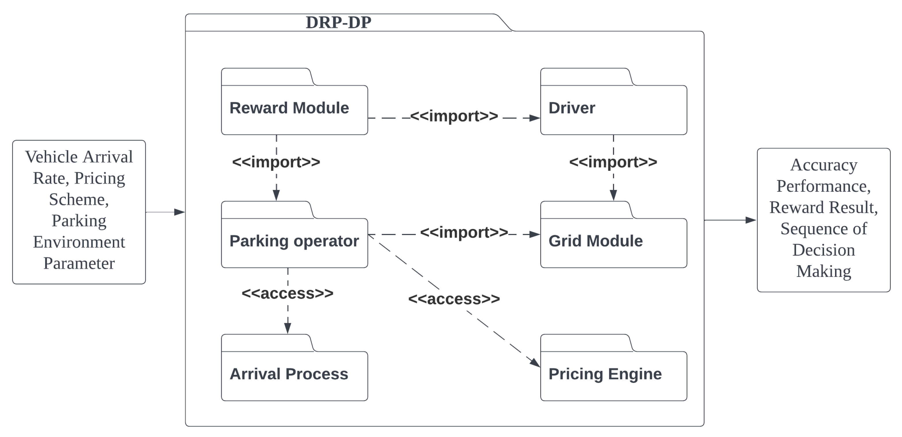
In this proposed solution, the dynamic pricing model is divided into different modules to perform different tasks. With the input of parking environments such as vehicle arrival rate and pricing scheme used by the target parking vendor, the model will produce accurate performance, reward results and sequence of decision making. Accuracy performance and reward results are used for the evaluation of DRL-DP, while a sequence of decision making assists the parking vendor to make a decision on price regulation. Figure 7 shows the modules and the corresponding tasks in the proposed method.

• Parking Operator An organisation that offers parking services is the parking operator. The capacity, pricing and location of the parking vendor will be specified. It will function as a player in this RL setting. The entity attribute such as capacity, price rate and location will refer to actual data collected from Location A and Location B.
• Driver The driver is an entity that requires a parking lot. The drivers can be classified as commuters (long-term), frequent visitors (medium-term) and intermittent visitors (short-term) [17]. The driver is defined by its current location, destination and preferences between price and distance (described as price-focused, balanced and distance-focused) [13]. The price and distance preference rates for the driver are normalised to a 0 to 1 interval. The higher the value, the higher the drivers’ preference. For the driver to decide which parking area to park his/her vehicle, this entity will calculate the preference score for each player and opponent. A lower score of preference will be chosen as the decided parking lot for the driver. The driver will be randomly initiated with a destination and starting location inside the defined grip boundary. The distance between the driver and the parking vendor will be pre-calculated by the grid module before the driver makes the decision.
• Grid Module The grid module is a two-dimensional (2D) Euclidean plane to represent the location of the parking operator and driver in the city’s urban area [13]. The 2D grip map refers to the geographic coordinate system using latitude and longitude. Each parking operator and driver will have their own location. The grid module consists of information about this parking area, such as road capacity, vehicle volume and direction. The grid module also calculates the distance between the driver and the parking vendor upon request from the driver.
• Pricing Engine The pricing engine fetches information about the parking service, such as the current pricing, the parking availability at the moment and the likelihood of the next arrival. According to the specified pricing scheme, such as arrival-time-dependent pricing (ATP), usage-aware pricing (UAP), and flat rate, the engine runs and designs new pricing for the next condition.
• Arrival Process SARIMAX is used to forecast the arrival of the vehicle at one-hour intervals using [21]. The forecasted arrival flow will be utilised in the RL simulation.
• Reward Module The reward module calculates the reward as environmental feedback of an action taken by the learning agent. The reward is calculated with the MDP and normalised to avoid bias.

3.2.3. Vehicle Flow Regulation

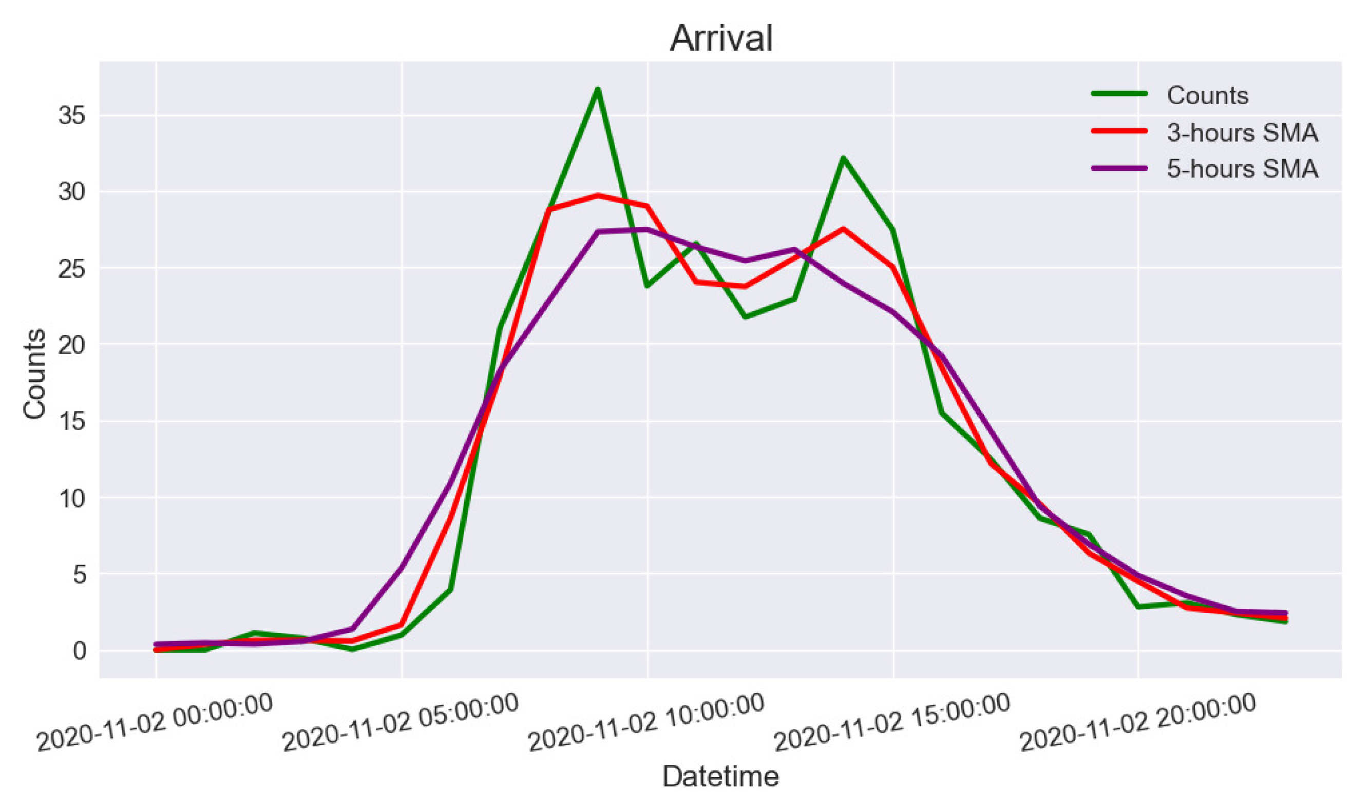
To alleviate the traffic congestion caused by a lack of vacant parking lots, smoothing the regression distribution model of vehicle arrival rate is the key to success. With smoothing the regression distribution model, a vehicle flow regulator is used to disperse the vehicle flow from peak hour to non-peak hour based on the historical parking occupancy rate. The simulated parking environment will use the regulated vehicle flow as a reference to calculate the reward at each time step. In this paper, the simple moving average (SMA) method is used as the vehicle flow regulator. It helps to identify the trend direction of the time series data. The local minimum and local maximum are moved towards the centre value by averaging the value in a moving window. The window represents a series of the number with the window width (number of observations used to calculate the moving average). The moving window slides along the time series data to calculate the average value. Given a set of numbers over a selected period of time, the SMA is extracted by calculating the arithmetic mean in these numbers as shown in Equation (1). In Equation (1), A_n indicates the number at period n, while n indicates the number of total periods. Figure 8 shows the result of vehicle arrival rate after the SMA.

$$SMA=\frac{A_1+A_2+...+A_n}{n}$$

(1)

3.2.4. Decision Maker

In this study, the driver acts as the decision maker, which affects the overall rewards returned in each time step of the episodes. The driver module makes a decision on the parking area and whether to visit the area or to shift to other time steps due to dynamic pricing adjustments.

Table 1. Notation used in driver decision making process.

Notation	Unit	Description
D	[0, …, 1]	Distance preference.
P	[0, …, 1]	Price preference.
O	[0, …, 1]	Occupancy preference.
LP	[lat, lng]	Location of the player.
LO	[lat, lng]	Location of the opponent.
LD	[lat, lng]	Location of the driver.
Ld	[lat, lng]	Location of driver’s destination.
DP, DO	[meter]	Distance from driver’s destination to the location of player and opponent.
PP, PO	[float]	Price of player and opponent.
SP	[float]	Sum of price of player and opponent.
OP, OO	[0, …, 1]	Parking occupancy of player and opponent.

shows the notation used in the driver decision-making process.

Every driver has his/her own preferred distance between the parking area and the destination D), parking lot price (P) as well as parking occupancy (O). The values for distance, price and occupancy preferences are normalised between 0 and 1. The distance and price preference pair uses preference value in common. For example, a price-preferred driver opts for a preference value of (0.7, 0.3) as they think highly of price. On the other hand, a distance-preferred driver prefers (0.3, 0.7), while a balanced-preferred driver uses (0.5, 0.5). Occupancy preference is a standalone option because it is common that drivers tend to avoid visiting a full parking area. The locations of player (L_P), opponent (_O), driver (L_D) and driver’s destination (L_d) are represented using latitude and longitude. D_P and D_O are the measured distances between the driver’s destination and the location of the player and opponent, these two values will be used in the equation of the driver to make a decision. P_P and P_O are the calculated prices if the driver parks at the parking area of the player and opponent. Equation (2) shows the decision-making process of the driver.

$$((D\ast D_P)+(P\ast \frac{P_P}{S_P})+(O\ast O_P))<((D\ast D_O)+(P\ast \frac{P_O}{S_P})+(O\ast O_O))$$

(2)

Equation (2) is divided into two parts. The first part on the left represents the player preference score, while the second part represents the opponent. The preference score is the total from the distance score, price score and occupancy score, and each will be normalised to 0 and 1 and multiplied by its preference value ratio.

3.2.5. Markov Decision Process (MDP)

Markov decision process (MDP) is a discrete-time stochastic control mechanism for modelling sequential decision making with state transition in a framework. At each time, the system might be in a different state. The decision maker makes an action in that state and the state transition will transfer from one state to another. The decision maker aims to seek a future state with the maximum reward. The proposed method is a partially observable Markov decision problem where the player only knows the opponent’s parking capacity, which is open to the public. The parking vendor does not have access to traffic information and the vehicle arrival rate throughout the simulation. Thus, the dynamic pricing problem is defined by the following components:

• Time step: Each time step represents a time over a finite time horizon from Monday to Sunday. It can be a different period section, such as morning, afternoon and night.
• State: To derive an intuitive state representation, it only contains the time step, the player’s parking occupancy and the opponent’s observable parking occupancy. The other predefined environment parameters such as parking capacity and parking pricing policy act as a constant value over the simulation.
• Observation: At every time step, the observation is done after the player performs an action. The vehicle arrival rate will be forecasted using SARIMAX. With the forecasted vehicle arrival rate, the driver simulates and performs decision making by observing the environmental variables such as parking fee and distance of parking vendor. The driver makes their decision on price and distance preferences. If there are rooms between the forecasted arrival rate and smoothed arrival rate, it will be declared as a controllable vehicle arrival. It will perform a decision on whether to continue parking or pay the next visit based on parking price and parking occupancy.
• Action: An action in the state is the discount performs at the current time step. The action is modelled as a fixed discount. The discount will be applied to the parking fee in the current time step.
• Transition: It is nondeterministic using the model-free RL methods for solving the parking problems. Thus, the transition moves from the current state to another state with the action taken.
• Reward: In this model, we consider multiple objectives: maximising parking occupancy rate, increasing parking revenue and traffic regulation result. Thus, the reward is obtained based on these objectives after taking an action in the state.

3.2.6. Deep Learning Model

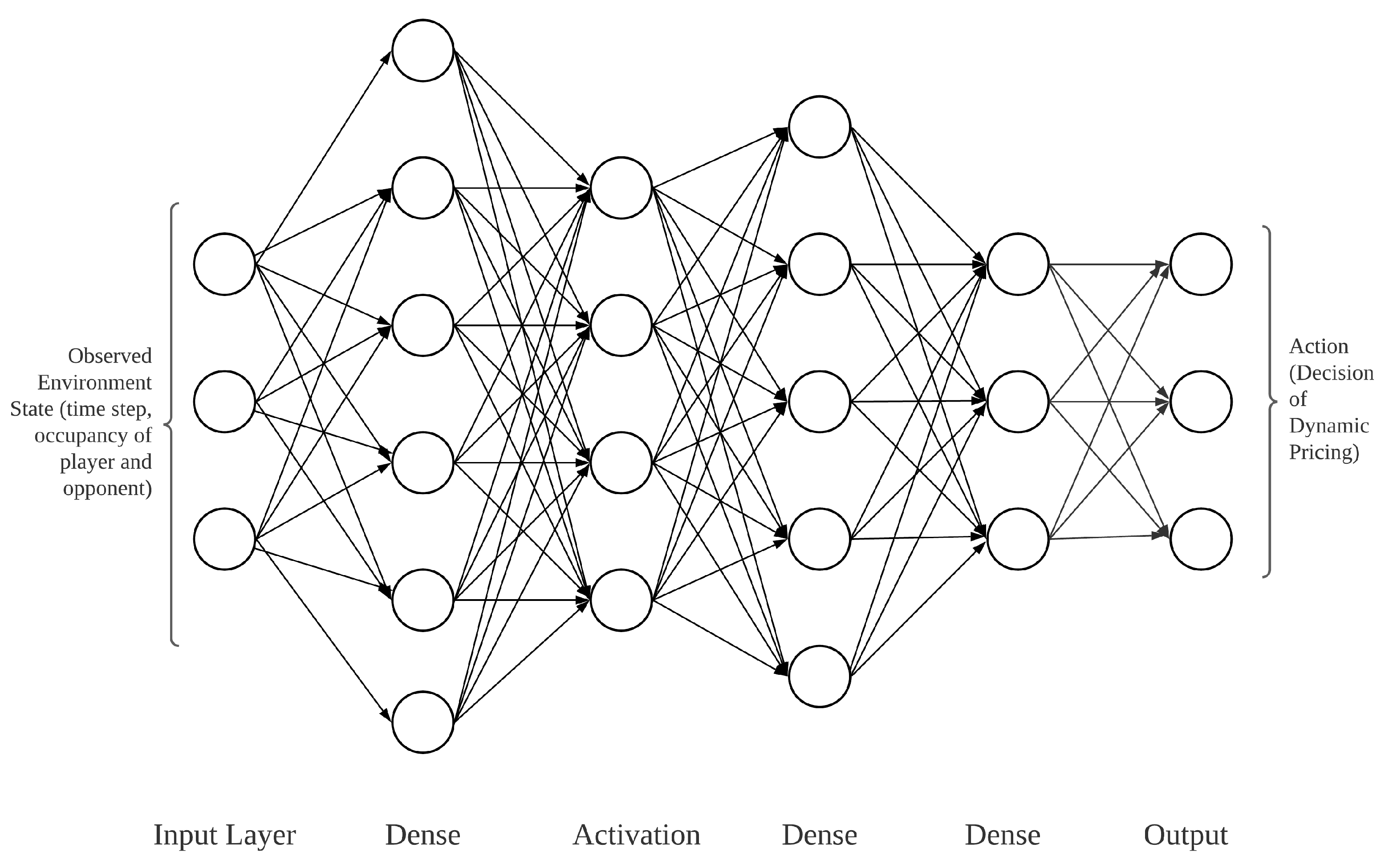
A deep neural network (DNN) is used in the proposed solution to learn from the environment observation and player action. The DNN model takes the environmental data such as time step and parking occupancy as the input variables and produces action as the output variable. The time step and parking occupancy of the parking vendor (player and opponent) are normalised as input for the DNN model. The model outputs the action with the maximum reward based on its historical training data.

Figure 9 depicts the architecture used in the DNN model. In the proposed solution, the environment data in each episode are produced from time to time. The DNN model is fit and updated every 200 episodes to achieve higher accuracy. In the simulations, an epsilon value is introduced to increase environment data exploration.

In the proposed method, we use an array consisting of the time step and parking occupancy rate of the player and opponent as the input layer because parameters such as pricing policies are updated based on the basis of the time step at each simulation.

Table 2. Parameters used in the DNN model.

Parameter	Variable	Unit	Description
Input layer	array	[0, …, 1]	An array consisting of the time step and parking occupancy rate of the player and opponent.
Activation	function	relu	Relu transforming weighted input layer to output layer.
First hidden layer	int	64	First hidden layer produces the output layer from the set of weighted input.
Second hidden layer	int	32	Second hidden layer produces the output layer from the set of weighted input.
Third hidden layer	int	16	Third hidden layer produces the output layer from the set of weighted input.
Output layer	array	[0, …, 1]	An array consisting of the result of the output of action space from the input time step.

shows the parameters used in the model. In each episode, the parking price is regulated based on the action taken. Hidden layers with 32 units and relu activation are used in the proposed method to achieve a faster processing speed. An output layer with 5 units is used following the number of actions in the action space.

3.2.7. Reinforcement Learning

The proposed model uses RL as a core mechanism to perform training from an environment based on rewarding desired price regulation and deep learning as a learning agent to learn and predict from the training dataset. Environment factors including traffic flow, parking availability and time step are received by the environment. The agent learns from interactive interaction within the environment. Figure 10 shows the general mechanism of the proposed RL mechanism.

As a real-world simulation to simulate a parking environment with a driver entity, the environment notation is important to demonstrate real-world behaviour and feedback.

Table 3. Notation of used variables in environment simulation.

Notation	Unit	Description
Y	(int)	Year.
M	(int)	Month.
D	(int)	Date.
t	(hour)	One hour interval.
T	(hour, …, hour)	A period of hours.
V	-	Parking vendor.
d	-	Driver.
Ld	(lat, lng)	Location of driver.
LP	(lat, lng)	Location of player.
LO	(lat, lng)	Location of opponent.
DP, DO	(meter)	Distance of driver’s destination to location of player and opponent.
FP, FO	(int)	Vehicle arrival flow rate of player and opponent.
FA	(int)	Vehicle arrival flow rate after SMA.
PP, PO	-	Pricing policies of player and opponent.
D(·)	-	Discount function.
N	(int)	Number of inflows.
NT	(int)	Number of inflows after SMA.
NC	(int)	Number of controllable inflows.

shows the notation of variables used in the environment simulation.

Y, M and D represent the environment datetime, $t\in T,T=\{0,1,\dots ,23\}$. T is a period of hours, while t is the component of T. V is the parking vendor that includes the player and opponents, while d represents the driver. L_d, L_P and L_O signify the locations of the driver, player and opponent, respectively. D_P and D_O are the distances between the driver’s destination and locations of the player and opponent. F_P and F_O are the vehicle arrival flow rates of the player and opponent, while F_A is the vehicle arrival flow rate after the SMA. P_P and P_O are the pricing policies of the player and opponent. On the other hand, D(·) denotes the discount function which returns the discount schema in the current time step and also acts as the action. N is the number of forecasted inflows in the current time step. N_T is the number of inflows after the SMA, while N_C is the controllable inflows which are obtained from the difference between N and N_T.

The Q-learning algorithm is a model-free off-policy reinforcement learning algorithm [22]. In the proposed method, the reward is obtained through a sequence of the driver’s decision making. A decision is made by the driver to park at a parking area to reflect the result of the action taken at each time step. The Q-table stores and updates the accumulated reward (q-value) at each time step. The Q-learning algorithm predicts the state-action combination based on a greedy policy where it takes the action with the maximum q-value in the Q-table. The learning agent studies to improve the reward by taking an action from the Q-table. In the proposed method, the epsilon-greedy policy is used. Exploration allows the agent to explore its knowledge to make a better action in the long term by avoiding choosing the maximum q-value and ignoring an action that has never been taken before. Exploitation allows the agent to exploit the current estimated maximum q-value and select the greedy approach. Exploration is increased using the epsilon value to avoid being trapped at a local optimum, as a trade-off between exploration and exploitation. An episode in this study refers to the selected week to undergo environment simulation. The episode will be repeated three thousand episodes to achieve learning efficiency and accuracy. The proposed approach is summarised in Algorithm 1.

The environment entity computes the entry and exit flow of the player and competitors in the reward function. The number of drivers will choose their parking space based on price and distance preference with the computed in and outflows. Algorithm 2 shows the procedure of the reward function.

Algorithm 1 Implementation of RL with Q-Learning for the parking industry.

1: Initialise environment variable (number of opponents, price range, datetime, period section and etc.) 2: Get the current time-step 3: N $\Leftarrow$ number of hours in period section (a period of hours) 4: while N > 0 do 5:       Gets an action based on the Q values of the Q-table. 6:       Performs the action 7:       Observe the environment and get the reward 8:       Update current state of environment 9:       Calculate new Q value and update to Q-table 10:      Increment the current time-step 11:      $N\Leftarrow N-1$ 12: end while

Algorithm 2 Proposed reward function to return reward at each time step.

1: Get player current state 2: Get opponent current state 3: Normalise vehicle stay time from player and opponent 4: Initialise rewards, in and out flow of vehicle to 0 5: $N\Leftarrow$ number of hours in period section (a period of hours) 6: while $N>0$ do 7:      Define hourly reward to 0 8:      $IN\_N\Leftarrow$ number of inflow of current hour (day and hour) 9:     $IN\_CN\Leftarrow$ controllable inflow by calculating the difference between target vehicle flow after vehicle flow regulation with forecasted inflow using historical parking occupancy data 10:    while $IN\_N>0$ do 11:          Initialise driver with stay time 12:          Driver makes decision on parking area 13:          Update reward value 14:          $IN\_N\Leftarrow N-1$ 15:     end while 16:     while $IN\_CN>0$ do 17:           Initialise driver with stay time 18:          Driver makes decision whether to park or visit next time and its parking area 19:          Update reward value 20:           $IN\_CN\Leftarrow N-1$ 21:      end while 22:      Update parking occupancy of player and opponent 23:      Add hourly reward to rewards 24:      Update occupancy of player and opponent 25:      Increment the current time-step 26:      $N\Leftarrow N-1$ 27: end while 28: Return rewards and updated environment data

4. Experimental Results

We present a series of experiments and simulations to assess the performance of the proposed method. In the parking industry, parking vendors in different parking areas aim at different types of visitors. For example, tourism areas usually target short-term visitors while office buildings used to have long-term visitors. Thus, test cases with different pricing policies are considered because they show competition among nearby parking vendors. The following shows the uniform arrivals in the simulations: (i) {“Begin”:0, “End”:4, “Fee”:4.0}, {“Begin”:5, “End”:10, “Fee”:10.0}, {“Begin”:11, “End”:17, “Fee”:8.0}, {“Begin”:18, “End”:24, “Fee”:6.0}; (ii) {“Begin”:0, “End”:24, “Fee”:10.0}. “Begin” indicates the beginning time boundary of the rate, “End” indicates the end time boundary of the rate, and “Fee” indicates the flat rate of the pricing policy. The following shows the progressive pricing in the simulations: (i) {“Unit”: 1.0, “Fee”: 3.0}, {“Unit”: 1.0, “Fee”: 2.0}, (ii) {“Unit”: 1.0, “Fee”: 5.0}, {“Unit”: 1.0, “Fee”: 3.0}, {“Unit”: 1.0, “Fee”: 2.0}. Unit indicates the unit of hour, while fee indicates the parking fee within the time, which means every X unit of hour cost Y. In the case of PP (i), one hour costs 3, two hours costs 5 and three hours costs 7, every one-hour increment will cost 2. Three sets of action spaces are designed for the parking vendors, and each action space contains five actions. By considering the big disparity of price range, the action space is set in a wider range to ensure rooms for the players to obtain better rewards. Some parking vendors use a relatively cheap pricing policy; thus some action spaces will provide price adjustments (rising in price) to get better rewards. The action spaces provided are: (i) [0, −5, −10, −15, −20], (ii) [−10, −5, 0, 5, 10], (iii) [−20, −10, 0, 10, 20]. For example, in action space [0, −5, −10, −15, −20], these five numbers are the selection to be taken by the player. Thus, each pricing policy pair of player and opponent will be repeated three times to obtain the results of using different action spaces under the same pricing policy pair. Each test case is tested using different reward approaches, including occupancy, revenue, traffic regulation performance and these three in union. The player updates the discount at each time step in the simulation. In the simulation, a time interval of one week is selected as the running episode for dynamic pricing. The combination of uniform arrival rate and progressive pricing will be simulated under three different action spaces. Each combination of pricing schemes used by the player and the enemy will be repeated three times with the different action spaces.

4.1. Evaluation for Occupancy Approach

This section evaluates the learning output of the proposed method using the occupancy approach. With a dynamic pricing model under the occupancy approach, training always worsens because there is limited capacity for each parking vendor. If the parking vendor aims to achieve a greater occupancy rate, he can always provide the greatest discount regardless of parking revenue. Thus, the parking lot will always be full, and the action taken (discount) will be meaningless. The deep learning agent always reaches a higher accuracy in the first 50 episodes because the learning agent easily reaches high accuracy with a random choice of action in this approach. However, the exploration will make the deep learning agent confused because sometimes it cannot get higher accuracy by selecting the greatest discount (action) since it does not have enough parking spaces for the upcoming vehicles.

Table 4. Accuracy performance under occupancy approach.

Experiment	Steps
	50	100	500	1000	2000	3000
	Accuracy
1	0.58	0.47	0.36	0.5	0.63	0.59
2	0.78	0.61	0.48	0.58	0.53	0.61
3	0.77	0.67	0.56	0.64	0.58	0.61
4	0.59	0.48	0.44	0.55	0.52	0.59
5	0.73	0.64	0.47	0.59	0.61	0.63
6	0.73	0.59	0.5	0.61	0.72	0.75
7	0.67	0.53	0.42	0.56	0.58	0.55
8	0.83	0.63	0.53	0.66	0.58	0.63
9	0.8	0.66	0.63	0.56	0.69	0.81
10	0.61	0.48	0.41	0.61	0.42	0.69
11	0.78	0.61	0.5	0.64	0.67	0.7
12	0.77	0.64	0.53	0.58	0.72	0.64
13	0.59	0.52	0.56	0.63	0.47	0.56
14	0.72	0.58	0.53	0.59	0.56	0.59
15	0.73	0.56	0.48	0.61	0.56	0.59
16	0.56	0.48	0.55	0.59	0.5	0.69
17	0.63	0.55	0.48	0.55	0.66	0.61
18	0.66	0.58	0.5	0.61	0.45	0.63
19	0.66	0.53	0.41	0.5	0.52	0.59
20	0.75	0.59	0.56	0.56	0.56	0.52
21	0.73	0.58	0.5	0.58	0.59	0.61
22	0.59	0.47	0.48	0.56	0.48	0.52
23	0.67	0.58	0.5	0.58	0.66	0.72
24	0.67	0.59	0.41	0.66	0.47	0.61
25	0.7	0.66	0.55	0.59	0.47	0.63
26	0.86	0.64	0.61	0.58	0.69	0.86
27	0.81	0.67	0.63	0.55	0.5	0.66
28	0.7	0.63	0.53	0.59	0.67	0.66
29	0.84	0.64	0.61	0.63	0.61	0.73
30	0.81	0.67	0.53	0.56	0.53	0.63
31	0.67	0.63	0.61	0.48	0.64	0.75
32	1	0.91	0.92	0.94	0.84	0.84
33	0.84	0.64	0.61	0.53	0.56	0.72
34	0.66	0.64	0.55	0.58	0.48	0.61
35	0.97	0.88	0.81	0.92	0.67	0.66
36	0.84	0.64	0.64	0.55	0.48	0.81
37	0.58	0.47	0.39	0.67	0.53	0.64
38	0.8	0.66	0.53	0.56	0.5	0.63
39	0.78	0.64	0.5	0.66	0.53	0.8
40	0.61	0.45	0.45	0.7	0.69	0.64
41	0.72	0.56	0.45	0.61	0.61	0.69
42	0.73	0.59	0.45	0.59	0.58	0.61
43	0.66	0.55	0.41	0.48	0.56	0.59
44	0.89	0.63	0.58	0.53	0.56	0.61
45	0.8	0.67	0.63	0.58	0.59	0.77
46	0.56	0.48	0.44	0.44	0.47	0.67
47	0.81	0.61	0.52	0.52	0.5	0.58
48	0.78	0.67	0.58	0.58	0.53	0.59

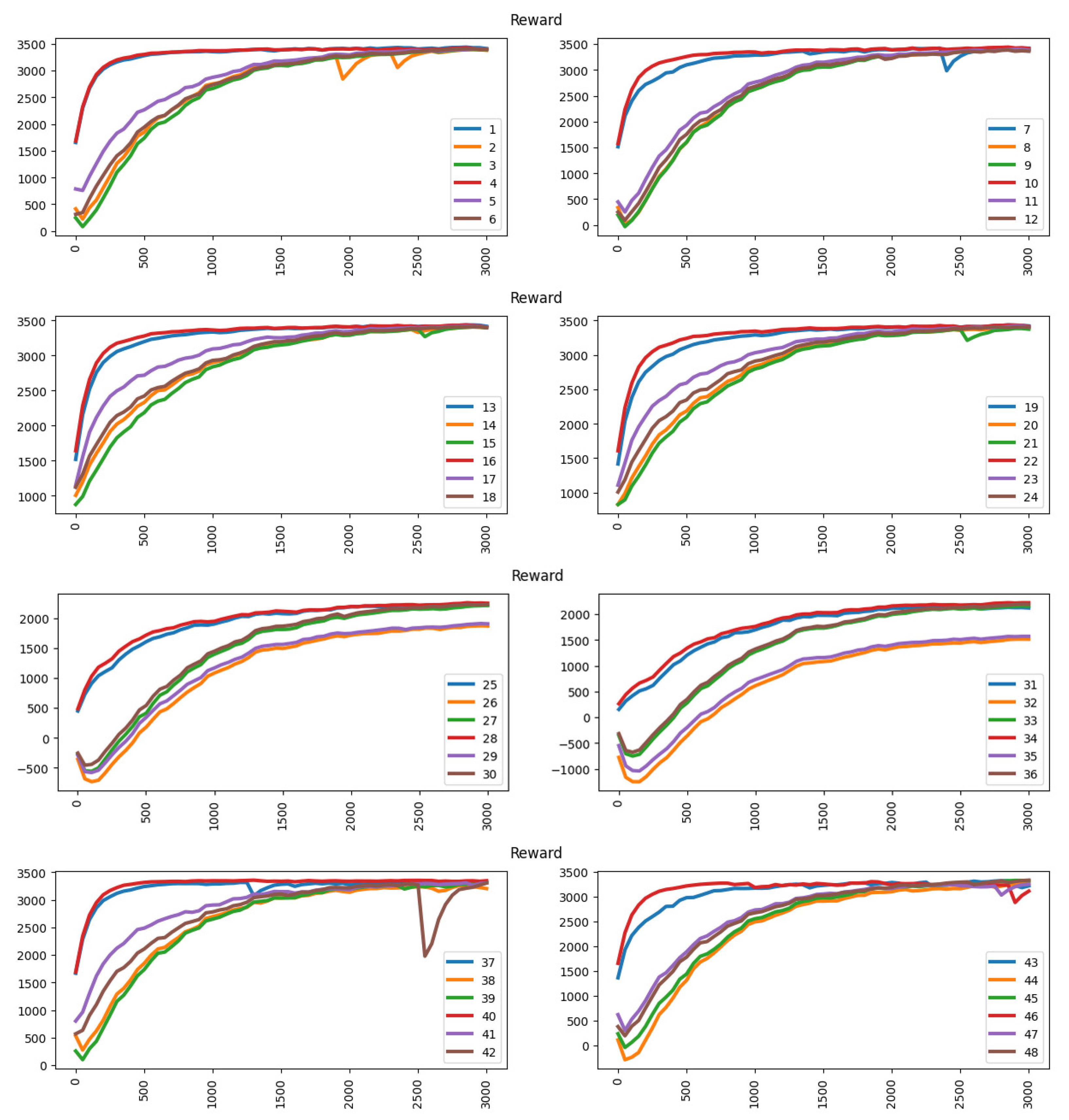
shows the accuracy performance under the occupancy approach. Figure 11 shows the reward performance under the occupancy approach. The dynamic pricing model always reaches an optimal value after around 2500 episodes.

4.2. Evaluation for Revenue Approach

This section compares the experiments using the revenue approach as the reward.

Table 5. Accuracy performance under the revenue approach.

Experiment	Steps
	50	100	500	1000	2000	3000
	Accuracy
1	0.97	0.88	0.92	0.88	0.89	0.86
2	0.77	0.66	0.66	0.69	0.69	0.73
3	0.53	0.59	0.83	0.7	0.72	0.91
4	0.98	0.88	0.98	0.92	0.98	0.75
5	0.78	0.7	0.77	0.56	0.78	0.66
6	0.83	0.81	0.84	0.75	0.88	0.69
7	0.83	0.7	0.56	0.86	0.92	0.92
8	0.78	0.78	0.83	0.92	0.88	0.83
9	0.48	0.58	0.73	0.63	0.8	0.59
10	0.92	0.88	0.89	0.86	0.88	0.86
11	0.78	0.81	0.75	0.66	0.58	0.94
12	0.48	0.59	0.75	0.69	0.78	0.91
13	0.98	0.91	0.86	0.98	0.89	0.86
14	0.78	0.58	0.69	0.55	0.42	0.7
15	0.8	0.66	0.63	0.52	0.42	0.64
16	0.98	0.92	0.92	0.86	0.97	0.89
17	0.84	0.75	0.58	0.58	0.53	0.67
18	0.81	0.66	0.63	0.5	0.63	0.56
19	0.98	0.88	0.91	0.84	0.91	0.92
20	0.77	0.67	0.64	0.56	0.5	0.56
21	0.8	0.73	0.58	0.53	0.55	0.81
22	0.98	0.88	0.91	0.84	0.95	0.83
23	0.86	0.66	0.64	0.58	0.69	0.72
24	0.8	0.7	0.61	0.58	0.45	0.73
25	0.98	0.89	0.92	0.89	0.73	0.91
26	0.95	0.88	0.89	0.84	0.75	0.91
27	0.92	0.94	0.92	0.78	0.78	0.83
28	0.98	0.88	0.89	0.92	0.86	0.91
29	0.89	0.8	0.86	0.84	0.77	0.91
30	0.94	0.8	0.92	0.78	0.8	0.81
31	0.56	0.56	0.5	0.73	0.72	0.77
32	0.55	0.56	0.52	0.72	0.63	0.61
33	0.47	0.63	0.59	0.75	0.72	0.72
34	0.7	0.78	0.63	0.77	0.67	0.7
35	0.63	0.67	0.66	0.64	0.72	0.72
36	0.66	0.78	0.69	0.77	0.77	0.75
37	0.97	0.88	0.97	0.89	0.88	0.84
38	0.67	0.73	0.63	0.61	0.64	0.83
39	0.58	0.61	0.84	0.67	0.7	0.89
40	0.98	0.88	0.89	0.89	0.89	0.95
41	0.8	0.67	0.69	0.5	0.7	0.84
42	0.81	0.69	0.75	0.63	0.61	0.73
43	0.84	0.73	0.7	0.81	0.83	0.86
44	0.61	0.69	0.73	0.83	0.8	0.86
45	0.56	0.53	0.59	0.7	0.78	0.81
46	0.91	0.8	0.89	0.8	0.77	0.92
47	0.84	0.7	0.67	0.58	0.63	0.77
48	0.56	0.78	0.81	0.63	0.7	0.91

shows the accuracy performance under the revenue approach. Figure 12 shows the reward results under the revenue approach. Under the revenue approach, the deep learning agent is able to achieve higher rewards in the training period. However, in some circumstances, the agent cannot get a higher reward such as in the ninth experiment. In the ninth experiment, the player has a pricing scheme with higher competitive power (cheaper than the opponent), so it is difficult to increase its competitive power by applying a discount. The action space used [−20, −10, 0, 10, 20] also restricts the player from getting a higher reward because the action space has an excessive gap because of each action. The player has difficulty increasing its competitive power, discount will cut off its revenue while rising in price will make it lose its competitive advantage. However, other experiments under the revenue approach can get higher rewards depending on the competitive power (pricing scheme and action space used in each experiment).

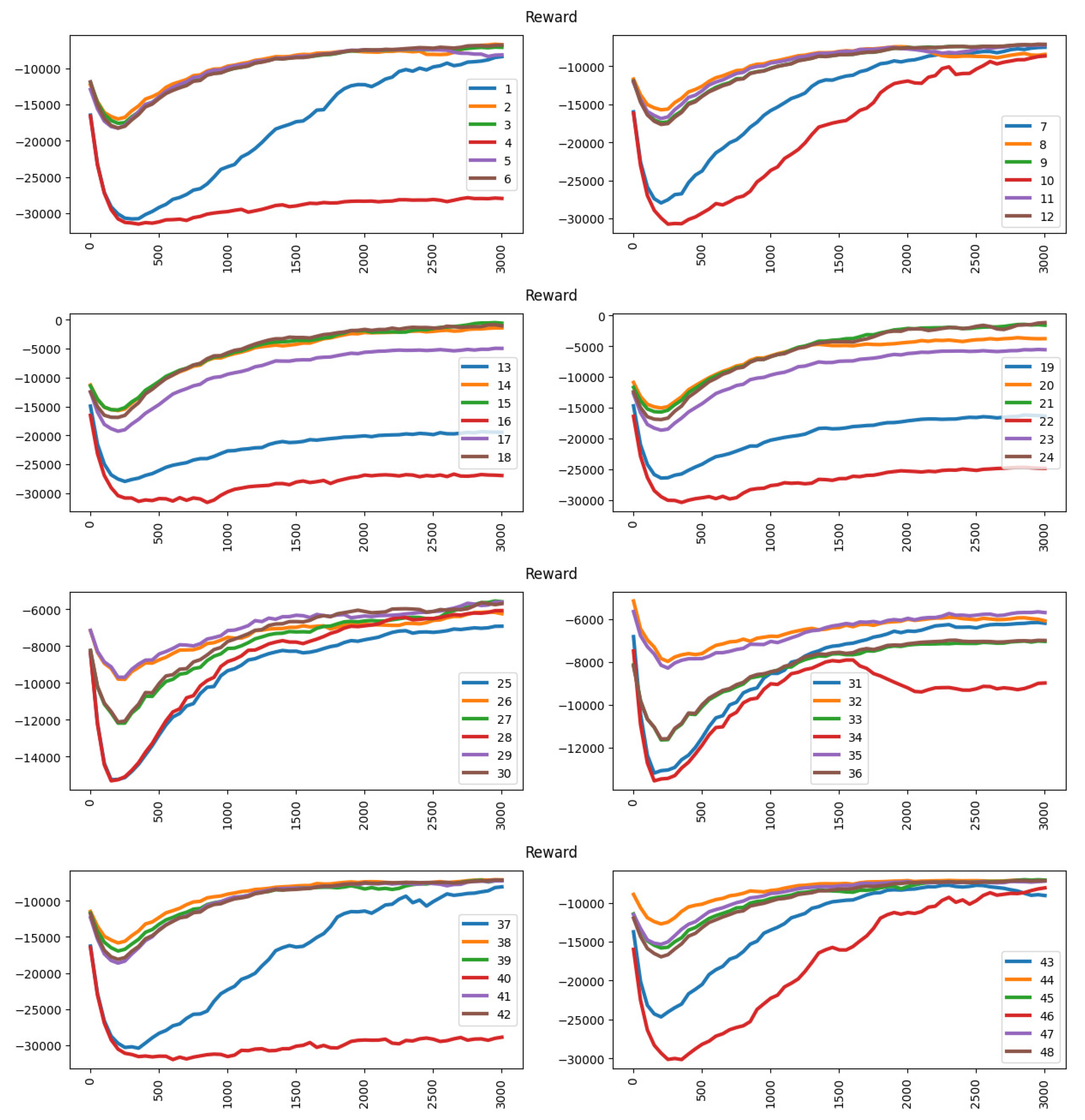
4.3. Evaluation for Vehicle Flow Regulation Approach

The experiment in this section compares learning output using the vehicle flow regulation approach. The deep learning agent learns to alleviate the vehicle flow during peak hours and enhance the vehicle flow during non-peak hours. When calculating the reward at each time step, the reward module use result from VFR (Section 3.2.3) as a reference, the nearer the target vehicle flow, the higher the reward, and vice versa.

Table 6. Accuracy performance under the vehicle flow approach.

Experiment	Steps
	50	100	500	1000	2000	3000
	Accuracy
1	0.5	0.55	0.56	0.44	0.56	0.56
2	0.5	0.55	0.58	0.53	0.55	0.47
3	0.52	0.47	0.48	0.47	0.53	0.45
4	0.48	0.55	0.5	0.55	0.56	0.44
5	0.53	0.45	0.58	0.45	0.53	0.41
6	0.52	0.56	0.55	0.45	0.53	0.53
7	0.56	0.52	0.55	0.55	0.64	0.38
8	0.52	0.55	0.44	0.42	0.56	0.45
9	0.52	0.55	0.55	0.53	0.53	0.53
10	0.48	0.53	0.42	0.52	0.58	0.52
11	0.5	0.55	0.58	0.41	0.44	0.44
12	0.52	0.47	0.56	0.61	0.58	0.48
13	0.52	0.47	0.55	0.5	0.56	0.48
14	0.45	0.58	0.73	0.42	0.86	0.97
15	0.59	0.56	0.77	0.58	0.83	0.92
16	0.53	0.53	0.53	0.36	0.5	0.44
17	0.48	0.64	0.72	0.7	0.86	0.77
18	0.47	0.56	0.61	0.5	0.63	0.97
19	0.58	0.52	0.61	0.45	0.61	0.55
20	0.42	0.5	0.69	0.52	0.73	1
21	0.59	0.55	0.73	0.64	0.67	0.73
22	0.53	0.52	0.5	0.55	0.58	0.48
23	0.48	0.63	0.72	0.59	0.66	0.72
24	0.45	0.55	0.64	0.44	0.41	0.61
25	0.58	0.5	0.58	0.67	0.72	0.58
26	0.63	0.53	0.56	0.61	0.56	0.72
27	0.42	0.59	0.39	0.64	0.5	0.44
28	0.58	0.53	0.55	0.7	0.61	0.63
29	0.58	0.53	0.56	0.64	0.52	0.75
30	0.44	0.61	0.58	0.61	0.56	0.55
31	0.63	0.58	0.55	0.61	0.69	0.69
32	0.61	0.55	0.58	0.63	0.7	0.8
33	0.56	0.48	0.56	0.56	0.69	0.56
34	0.63	0.59	0.61	0.69	0.8	0.67
35	0.61	0.56	0.63	0.66	0.89	0.91
36	0.55	0.53	0.58	0.48	0.64	0.67
37	0.55	0.56	0.59	0.45	0.53	0.48
38	0.48	0.59	0.52	0.52	0.58	0.47
39	0.52	0.48	0.58	0.39	0.58	0.55
40	0.55	0.56	0.56	0.61	0.58	0.5
41	0.52	0.55	0.53	0.44	0.45	0.44
42	0.52	0.53	0.56	0.55	0.59	0.45
43	0.55	0.5	0.63	0.45	0.53	0.47
44	0.53	0.53	0.55	0.52	0.52	0.55
45	0.52	0.55	0.53	0.52	0.55	0.56
46	0.48	0.56	0.59	0.59	0.55	0.47
47	0.5	0.5	0.55	0.52	0.56	0.47
48	0.52	0.47	0.58	0.42	0.48	0.42

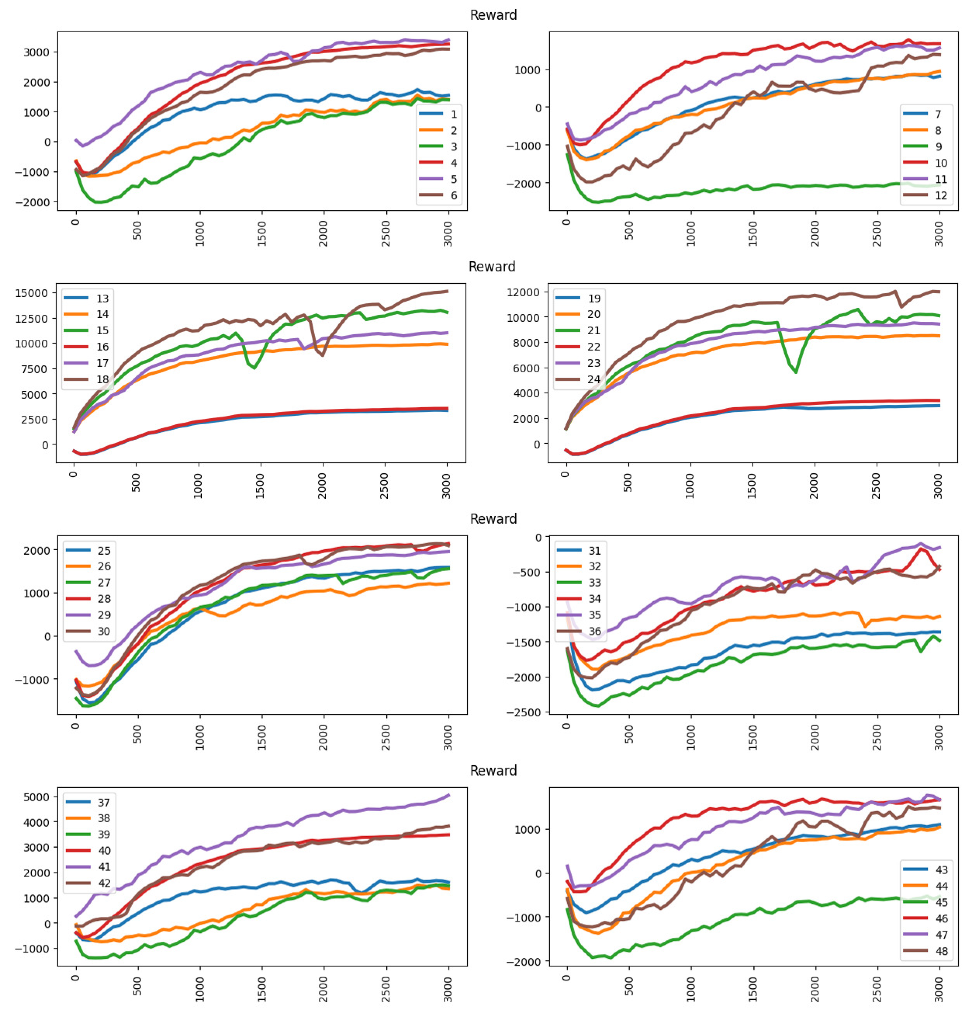
shows the accuracy performance under the vehicle flow regulation approach. The accuracy performance under the vehicle flow regulation approach is barely satisfactory. However, the reward result increases under some circumstances. Figure 13 shows the reward result under the vehicle flow regulation approach. When there are significant disparities of competitive power among parking vendors, the deep learning agent finds it difficult to achieve higher rewards, such as in the 1st, 4th, 7th, 13th, 16th, 19th, 22nd and 40th experiments. In those experiments, the player uses a cheaper pricing scheme (higher competitive power) with action space [0, −5, −10, −15, −20] (only discount without rising in price). The action space used in those experiments will increase its competitive power (or remain the same). Thus, it cannot decrease the vehicle arrival rate by price regulation.

4.4. Evaluation for Occupancy, Revenue and Vehicle Flow Regulation (Unified) Approach

The experiment in this section compares the learning output using the union approach which included occupancy, revenue and vehicle flow regulation.

Table 7. Accuracy performance under the occupancy, revenue and vehicle flow regulation (unified) approaches.

Experiment	Steps
	50	100	500	1000	2000	3000
	Accuracy
1	0.53	0.5	0.69	0.7	0.92	0.77
2	0.63	0.47	0.58	0.55	0.47	0.69
3	0.58	0.56	0.56	0.47	0.59	0.66
4	0.52	0.53	0.55	0.56	0.66	0.53
5	0.44	0.59	0.61	0.56	0.55	0.7
6	0.58	0.58	0.58	0.53	0.52	0.66
7	0.61	0.56	0.77	0.75	0.94	0.91
8	0.56	0.47	0.63	0.56	0.48	0.7
9	0.58	0.56	0.53	0.56	0.59	0.58
10	0.52	0.5	0.66	0.7	0.89	0.98
11	0.61	0.58	0.58	0.58	0.64	0.83
12	0.58	0.56	0.56	0.58	0.64	0.7
13	0.58	0.56	0.61	0.64	0.66	0.56
14	0.81	0.66	0.86	0.7	0.89	0.94
15	0.77	0.56	0.72	0.75	0.44	0.59
16	0.5	0.48	0.56	0.56	0.55	0.39
17	0.69	0.67	0.81	0.77	0.83	0.91
18	0.86	0.7	0.75	0.7	0.73	0.92
19	0.58	0.58	0.7	0.59	0.69	0.66
20	0.7	0.58	0.83	0.67	0.95	0.95
21	0.58	0.5	0.81	0.67	0.91	0.77
22	0.52	0.53	0.55	0.59	0.5	0.52
23	0.66	0.69	0.81	0.77	0.67	0.86
24	0.78	0.69	0.77	0.78	0.7	0.78
25	0.55	0.63	0.7	0.56	0.88	0.94
26	0.53	0.56	0.44	0.55	0.47	0.88
27	0.5	0.58	0.55	0.36	0.48	0.47
28	0.58	0.66	0.7	0.59	0.94	0.69
29	0.52	0.58	0.52	0.39	0.61	0.86
30	0.5	0.61	0.52	0.61	0.56	0.83
31	0.58	0.45	0.5	0.7	0.77	0.64
32	0.56	0.53	0.34	0.52	0.58	0.5
33	0.52	0.56	0.45	0.42	0.5	0.56
34	0.58	0.47	0.48	0.69	0.78	0.86
35	0.56	0.53	0.52	0.55	0.64	0.84
36	0.53	0.56	0.41	0.53	0.55	0.48
37	0.53	0.52	0.66	0.75	0.61	0.89
38	0.53	0.48	0.59	0.5	0.48	0.45
39	0.53	0.56	0.59	0.63	0.58	0.48
40	0.52	0.55	0.48	0.41	0.56	0.48
41	0.39	0.64	0.69	0.52	0.67	0.52
42	0.59	0.48	0.59	0.5	0.69	0.59
43	0.63	0.63	0.8	0.69	0.56	0.53
44	0.53	0.53	0.53	0.48	0.59	0.67
45	0.52	0.53	0.55	0.52	0.47	0.44
46	0.52	0.52	0.66	0.69	0.64	0.69
47	0.56	0.58	0.66	0.48	0.59	0.67
48	0.55	0.53	0.59	0.56	0.48	0.59

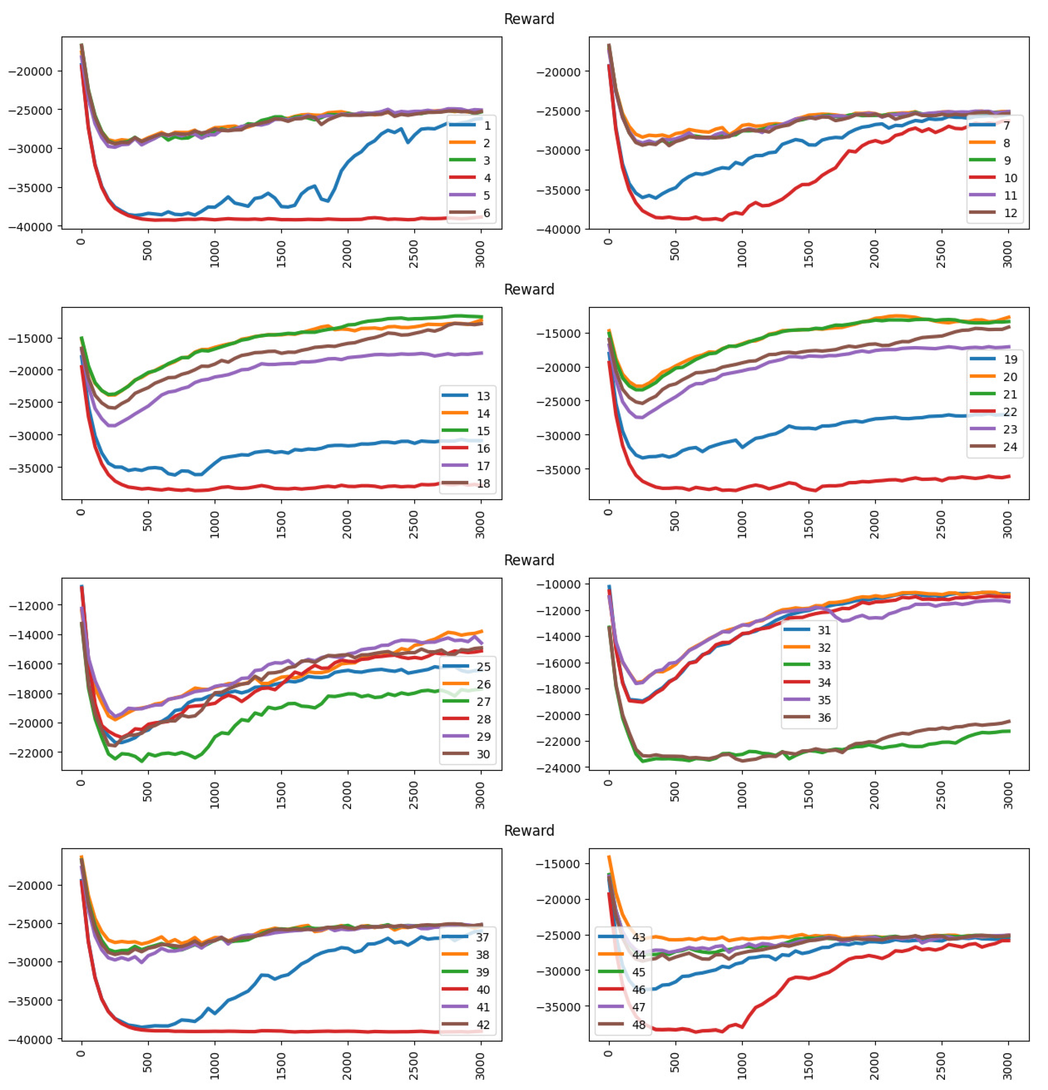
shows that the accuracy performances under the unified approach are barely satisfactory. Figure 14 shows the reward result under the unified approach. This may be caused by the occupancy, revenue and vehicle flow regulation approaches being influenced by each other, which makes it harder to achieve higher accuracy. Nevertheless, the deep learning agent is achieving higher rewards in the training period.

4.5. Discussion

So far, we have performed the experiments using different approaches such as parking occupancy and revenue. The same pricing schema and discount action space settings are used for these approaches to evaluate the accuracy and learning efficiency of the learning algorithm. Since the scale varies between each other, these approaches also show different tendencies in the learning output. From the experiment observations, some discussions can be concluded. The average reward fluctuated greatly during the training period [1, 100], and it slowly converged to an optimal point (highest reward based on its approach) where the exploration reduced at this training period and the exploitation starts to stabilise. The exploration can help to avoid the learning agent from being biased towards short-term gains. The optimal value of the experiments varies for different pricing schemas. This might be caused by the competitive power of the player compared to competitors in the parking market.

The higher the price adjustment range in the action space, the higher the variation of the average reward. This is because a higher price adjustment range represents a higher possibility to change the driver’s preference. For example, the action space [−20, −10, 0, 10, 20] enables the player to make greater adjustments to the pricing schema. When the player uses the uniform arrival rate (UA), the action space must be precise and narrow because the high difference value is an obstacle for the learning agent to improve the reward. This might be solved by using a more precise and complex action space for the player. When the player uses a low-priced pricing policy, the player needs to raise the price to increase the revenue reward. Otherwise, the revenue of the player is difficult to increase because the action taken as a discount will only increase the parking occupancy rate, not help in increasing revenue.

Under the occupancy approach, the learning agent can reach an optimal reward easier by selecting the best action because the player loses sight of the parking revenue. Under the revenue approach, the learning agent can reach an optimal value except when the player uses a low-priced pricing policy and the action space without a higher price. The vehicle flow is much more difficult to regulate as compared to the occupancy and revenue approaches because the low parking price will distract the drivers and vice versa.

5. Conclusions

This study examines a dynamic pricing mechanism for the parking sector based on parking income and vehicle arrival rate. The parking industry’s dynamic pricing model is then put out and studied using reinforcement learning. It is demonstrated that the dynamic pricing method works well to arrive at the best outcome.

However, there are still some problems to be solved, such as on-street parking and facility impacts. The amount of on-street parking may affect the willingness of the driver to park at off-street parking (parking vendor with barrier-gate) because of the difference in price. Moreover, the building type of the parking premise will also affect the drivers’ parking willingness if their destination is a tenant or a shop in the opponent’s building. More human factors such as driver’s preference based on parking area also provide a high impact on dynamic pricing. The driver’s preference may be affected by the type of parking area such as tourism, office and residential area.

For future improvements, some important aspects have to be taken into account in order to provide a more accurate and reliable result. Vehicle volume on the road is a critical factor to influence vehicle arrival rate, especially in urban areas because vehicle volume on the road may affect the ability of the driver to find a parking lot. Thus, the relationship between vehicle volume and vehicle arrival rate in the parking area has to be observed and analysed to provide a more sophisticated parking environment simulation. Thus, future works may focus on customising flexible environment parameters to adapt to complicated real-world environments.