Variational Bayes to Accelerate the Lagrange Multipliers towards the Dual Optimization of Reliability and Cost in Renewable Energy Systems

Abstract

Renewable energy sources are constantly increasing in the modern power systems. Due to their intermittent and uncertain potential, increased spinning reserve requirements are needed to conserve the reliability. On the other hand, each action towards efficiency improvement and cost reduction contradicts the participation of variable resources in the energy mix, requiring more accurate tools for optimal unit commitment. By increasing the renewable contribution, not only does the overall system inertia decrease with the decreasing conventional generation, but more generators that are expensive are also introduced. This work provides a radically different approach towards a tractable optimization task based on the framework of Lagrange relaxation and variational Bayes. Following a dual formulation of reliability and cost, the Lagrange multipliers are accelerated via a machine learning mechanism, namely, variational Bayesian inference. The novelty in the proposed approach stems from the employed acquisition function and the effect of the Gaussian process. The obtained results show great improvements compared with the Lagrange relaxation alternative, which can reach over USD 1 M in production cost credits at the least number of function evaluations. The proposed hybrid method promises global solutions relying on a proper acquisition function that is able to move towards regions with minimum objective value and maximum uncertainty.

1. Introduction

Under the consequences of one of the biggest energy crises, all countries around the globe are exploring viable solutions for alternatives to fossil fuels and especially natural gas. In the light of polluting emissions and climate change, the necessity of renewable energy sources (RES) grew exponentially during the last two years, under the shadow of a war that is still plaguing European countries and states around the world. Apart from the public concerns relating to the upcoming living conditions, a huge uncertainty has been added to the price of essential products that are either directly or indirectly affected by the dependency on imported natural gas [1].

As more stakeholders seek greater clarity and confidence in long-term investments and their respective opportunities in the forthcoming years, the impact of a potential integration of renewable and storage systems needs to be evaluated. To mitigate the environmental concerns around fossil fuels exploitation, the benefit list of a transition towards sectors electrification, de-carbonization and sustainability must be strengthened, facilitated by efficient tools that are able to consolidate the real-world constraints. Recent research activities on renewable sources and storage have been concentrated successfully on single operations and objectives. New objectives have recently appeared, targeting the co-optimization of cost, emissions, security and reliability within the power systems. These targets can be examined in depth, considering resources hybridization, multi-sectoral energy satisfaction and smart grid consolidation. As the missing link between intermittent renewable power and constant reliability, the various energy storage technologies can be compared, accounting for microgrid and virtual power plant formations.

The current state of research carefully reviews and assesses various approaches in optimal unit commitment (UC), which forms one of the most important tasks of the modern electric industry. Empirical methods simply consider the satisfaction of load by adjusting electricity production to demand during normal conditions [2,3]. In the case of generation deficits, load shedding takes place, while during excess generation, the electricity from RES is curtailed. More evolutionary methods aim at the co-optimization of load shedding and RES curtailment, following a priority with respect to generating the incremental cost of the participating units [4]. In this direction, priority-list schemes [5], Benders decomposition [6], Branch-and-Bound [7] and Lagrange relaxation (LR) [8] are some representative techniques that are able to offer only near-optimal solutions. Their relevant advantages rely on the mathematical process, which facilitates both the traceable transitions towards the final recommendation and the computational complexity irrespective of the number of examined generators. On the other hand, the obtained duality gap cannot be eliminated due to the imposed, real-world constraints that plague the generation activity today. These refer to the complicating constraints of power balance and spinning reserve in order to deal with the intermittent and stochastic behaviour of RES [9].

To offer adaptive mechanisms that are able to satisfy the required ramping capability, unit capacity and operating times, a heuristic search has been proposed in several research works. These approaches rely on physical- or biological-based algorithms and involve genetic algorithms [10], particle swarm optimization [11], simulated annealing [12], ant colony [13], tabu search [14] and so on. Although flexible, these techniques cannot guarantee optimality, especially in large systems where the magnitude of their sub-optimality cannot be evaluated [15]. As a result, the most recent version of UC solvers includes meta-heuristic alternatives. Binary grey wolf [16], binary whale [17], binary successive civilized swarm optimization [18], binary fish migration [19], binary cuckoo search [20], binary differential evolution [21], binary moth flame [22], coyote [23], binary [24] and artificial bee colony [25], monarch butterfly [26] and sine-cosine variant [27] are only some of the optimization approaches that exploit the merits derived from mathematical and heuristic methods to hybridize the process with one critical goal—to provide optimal exploration–exploitation trade-offs. This way, the last category aims at providing near-optimal solutions to the UC, consolidating several complicating equality and inequality constraints, conditional limitations and space boundaries while examining a large number of participating generating units over different time horizons. However, together with heuristics, meta-heuristic methods involve randomness and use the stochastic (or fuzzy) approach in moving from one solution to another [28].

To ameliorate for the demerits arising from the aforementioned approaches involved in emerging UC proposals, this work exploits the most recent advancements of the Lagrange framework and Bayesian inference to develop a radically new optimization tool for optimal UC schedules. Using the duality gap theory to form a Lagrangian objective, the problem is repeatedly minimized by updating the Lagrange multipliers based on Bayesian optimization. The multipliers account for both the security (power balance) and reliability (spinning reserve). The proposed approach essentially improves the computational performance via the dual optimization of reliability and cost in systems with highly variable resources. In addition, it offers global explorations in a minimum number of function evaluations, ensuring the transparency between the recommended solutions. The innovation in the proposed approach stems from the employed acquisition function and the effect of the Gaussian process. In this way, the expected improvement function properly guides optimization towards regions with either a minimum, mean or maximum uncertainty.

The rest of the paper is organized as follows. In Section 2, the dual formulation of the problem is presented, along with the complicating and unit-specific constraints. Section 3 deals with the mathematical formulation of Lagrange relaxation and variational Bayes as the primer for Lagrange-multipliers acceleration towards rapid convergence. The experimental evaluation is included in Section 4, where the obtained results are discussed in detail. Finally, the conclusions are drawn in Section 5.

2. Dual Problem Formulation

In its most analytical form, the objective of the unit commitment task is formulated to minimize the total generation cost (TGC), considering three main expenses. First, the fuel consumption cost $F\left(S,P\right)$ is estimated based on the dynamic state ($S_i^t$) and actual power output ($P_i^t$) of each committed generator i during the time interval t. This expenditure relies on the cost coefficients of each independent generator, which in turn accounts for the heat rate coefficients (a_i, b_i, c_i) and fuel specific cost f_c. The following quadratic equation is generally used to define these expenses.

$$F\left(S_i^t,P_i^t\right)=S_i^t\left\{f_c\left[a_i{\left(P_i^t\right)}^2+b_i{P}_i^t+c_i\right]\right\}$$

(1)

The second aspect regards the emission cost $E\left(S,P\right)$ that evaluates the gaseous emissions from different pollutants, including carbon dioxide (CO₂), carbon oxide (CO), nitrogen oxides (NO_x), sulfur oxides (SO_x) and other hydrocarbon byproducts (C_xH_y). Assuming the emission cost coefficients (e_i1, e_i2, e_i3) of each generator, the following equation can be utilized to account for this expenditure [29].

$$E\left(S_i^t,P_i^t\right)=S_i^t\left[e_{i1}{\left(P_i^t\right)}^2+e_{i2}{P}_i^t+e_{i3}\right]$$

(2)

The last portion of costs refers to the penalties (Π_t of Equation (3)) and deteriorates reliability. This relates the energy not-served (P_ENS), translated as load shedding, the spinning reserve not-served (P_SRNS) and the curtailed power from RES (P_cut-RES) with their respective penalty costs of π_E, π_SR and π_RES [4].

$${\mathsf{\Pi }}^t={\pi }_{{\rm E}}{P}_{ENS}^t+{\pi }_{SR}{P}_{SRNS}^t+{\pi }_{RES}{P}_{cut-RES}^t$$

(3)

Finally, a factor is added to both unit-specific costs to include the start-up cost with respect to fuel consumption (FSU_i) and associated emissions (ESU_i). The comprehensive objective can now be represented with the aid of Equation (4), considering a time horizon T and participating generators N.

$$TGC={\displaystyle \sum _{t=1}^T}\left\{{\displaystyle \sum _{i=1}^N}\left[F\left(S_i^t,P_i^t\right)+E\left(S_i^t,P_i^t\right)+S_i^t\left(FS{U}_i+ES{U}_i\right)S_i^{t-1}\right]+{\mathsf{\Pi }}^t\right\}$$

(4)

The complicating constraints of the UC objective give priority to every action towards emissions inclination, efficiency improvement and RES integration. To this end, the power equilibrium expresses the equality constraints such that:

$${\displaystyle \sum _{i=1}^N}{S}_i^t{P}_i^t=P_{net}^t , \forall t\in T$$

(5)

$$P_{net}^t=P_{load}^t-P_{VRES}^t$$

(6)

$$P_{VRES}^t=P_{PV}^t+P_{wind}^t+P_{biomass}^t+P_{water}^t+P_{geo}^t+P_{CHP}^t+P_{FC}^t$$

(7)

While the net load ($P_{net}^t$) equals the residual demand after the variable RES ($P_{VRES}^t$) involvement, the contribution of solar PVs ($P_{PV}^t$), wind ($P_{wind}^t$), biomass ($P_{biomass}^t$), hydro and water alternatives such as wave and tidal ($P_{water}^t$), geothermal ($P_{geo}^t$), combined heat and power ($P_{CHP}^t$) and fuel cells using renewable fuels ($P_{FC}^t$) for electricity demand satisfaction requires increased spinning reserves (SR^t) to conserve the system’s reliability. These requirements are represented by the following inequality constraint:

$${\displaystyle \sum _{i=1}^N}{S}_i^{t}R{U}_i^t\ge S{R}^t , \forall t\in T$$

(8)

To adequately respond to probable, sudden deviations between actual and forecasted values, for both the demand and VRES contribution, the ramp-up capability ($R{U}_i^t$) from all committed generators during the interval t must satisfy the following requirements [30]:

$$S{R}^t={\xi }_{load}{P}_{load}^t+{\xi }_{VRES}{P}_{VRES}^t$$

(9)

In order to account for the unit-specific and plant-wide constraints, the limitations of power capacity, ramping capability, minimum state-change periods and compulsory status are taken into consideration. The power-output boundaries for each generator are shown in Equation (10). The positive (RU_i) and negative (RD_i) rate of change of the power output are presented with Equations (11) and (12). Equations (13) and (14) are used to calculate the minimum time (MU_i) that must be elapsed before a generating unit can switch from on-status to off-status ($S_i^t=1\to 0$) and vice versa (MD_i). The unavailability of a generator due to an unintentional failure or intentional maintenance is translated as a “must out” value. On the contrary, based on security and stability issues, at least one unit has to operate in “must run” within each independent power plant. Combined cycle units possess an exception and interchange between these states according to their mode of operation. Consequently, each mode is expressed via a different quadratic function, the state of which becomes “on” only when called upon [31].

$$P_{i,min}\le P_i^t\le P_{i,max} ,\forall t\in T$$

(10)

$$P_i^t-P_i^{t-1}\le R{U}_i ,\forall t\in T$$

(11)

$$P_i^{t-1}-P_i^t\le R{D}_i ,\forall t\in T$$

(12)

$${\displaystyle \sum _{t=t_{on}}^t}{S}_i^t\ge M{U}_i ,\forall t\in T$$

(13)

$${\displaystyle \sum _{t=t_{off}}^t}\left(1-S_i^t\right)\ge M{D}_i ,\forall t\in T$$

(14)

$$S_i^t=\{\begin{array}{ll}0 ,& if i=must out\\ 1 ,& if i=must run\end{array} ,\forall t\in T$$

(15)

The plant-wide restriction (c_p) regards the maximum number of actions that can simultaneously be performed within a power plant. It is reflected by the maximum number of system operators and/or the capability of the integrated auxiliary equipment. The so-called crew constraint is formulated as:

$$c_p={\displaystyle \sum _{i=1}^{N_p}}{S}_i^t\left(1-S_i^{t-1}\right) ,\forall t\in T$$

(16)

where N_p is the number of generating units within the power plant p.

3. Mathematical Framework

In this section, the mathematical framework relating to the algorithm developed for global optimization is presented and explained in detail. The objective function is expressed as Lagrangian, and the UC problem is decomposed into sub-problems that are coupled by making use of Lagrangian multipliers. In this way, the constrained optimum can be obtained through the dual optimization of reliability and cost, which can manifest as spinning reserve satisfaction and power balance.

3.1. Lagrange Relaxation Approach

The Lagrangian function can be written with respect to the non-negative multipliers of λ^t and μ^t as:

$$ℒ=F\left(S_i^t,P_i^t\right)+{\displaystyle \sum _{t=1}^T}{\lambda }^t\left(P_{net}^t-{\displaystyle \sum _{i=1}^N}{S}_i^t{P}_i^t\right)+{\displaystyle \sum _{t=1}^T}{\mu }^t\left[P_{net}^t+S{R}^t-{\displaystyle \sum _{i=1}^N}{S}_i^t\left(P_i^t+R{U}_i\right)\right]$$

(17)

To separately minimize the contribution of each generating unit, Equation (17) is rewritten in the following form:

$$ℒ={\displaystyle \sum _{i=1}^N}{\displaystyle \sum _{t=1}^T}\left\{S_i^t\left[F\left(S_i^t,P_i^t\right)+\left(1-S_i^{t-1}\right)FS{U}_i\right]-{\lambda }^t{S}_i^t{P}_i^t-{\mu }^t{S}_i^t{P}_i^t\right\}+{\displaystyle \sum _{t=1}^T}\left[{\lambda }^t{P}_{net}^t+{\mu }^t\left(P_{net}^t+S{R}^t\right)\right]$$

(18)

At this stage, the complicating constraints can temporarily be ignored, and the first term of the expression can be minimized based on the problem:

$$\underset{S_i^t,P_i^t}{min}\dot{ℒ}={\displaystyle \sum _{i=1}^N}min{\displaystyle \sum _{t=1}^T}\left\{S_i^t\left[F\left(S_i^t,P_i^t\right)+\left(1-S_i^{t-1}\right)FS{U}_i\right]-{\lambda }^t{S}_i^t{P}_i^t-{\mu }^t{S}_i^t{P}_i^t\right\}$$

(19)

This is subject to the constraints (10)–(15). By eliminating the coupling constraints, a guaranteed solution is expected if the constrained optimization task forms a relaxed problem that offers a lower bound to the original problem [32]. In the Lagrange relaxation method, the separability of the constraints is the underlying assumption that allows for the violation penalization towards optimality. Denoting with s^k the mismatches of the coupling constraints at iteration k, the vector of Lagrange multipliers is updated considering the sub-gradient method as follows [9]:

$$\left[{\lambda }^{k+1} {\mu }^{k+1}\right]=\left[{\lambda }^k {\mu }^k\right]+a^k\frac{s^k}{||s^k||}$$

(20)

$$a_k=\frac{1}{\alpha +\beta k}$$

(21)

The terminating criterion is called a duality gap (ε) and shows the difference percentage between the primal (J) and the dual (q) problem, respectively, according to Equation (22).

$$\epsilon =\frac{J-q}{\left|J\right|}\le error$$

(22)

The repeating procedure stops when ε becomes lower than either a pre-specified tolerance (error) or a maximum number of defined iterations. Although the sub-gradient method is simple and computationally non-intensive, the oscillating behavior makes it difficult to design an appropriate stopping criterion. Typical solutions propose different step-size values for the over-constrained and under-constrained conditions at the expense of the exploration-space decrease and convergence time. In addition, unlike linear programming, integer linear programming cannot provide a strong duality theory. In this way, the optimal value of the dual Langrangian problem does not have to be the same as the optimal value of the original (primal) problem, which implies that the magnitude of the sub-optimality is controversial [33].

3.2. Bayesian Primer

To overcome the drawbacks of the weak duality and the oscillatory behavior of Lagrange relaxation, the Lagrange multipliers are modeled to form a Gaussian process. This constitutes a stochastic process that governs the properties of functions rather than describing random variables, which are scalars or vectors. Consequently, the new population is produced by adding the Gaussian number $\mathcal{N}\left(0,{\sigma }^2\right)$ with a mean of zero and a pre-determined standard deviation to each multiplier such that:

$${\lambda }^{k+1}={\lambda }^k+\mathcal{N}\left(0,{\sigma }^2\right)$$

(23)

$${\mu }^{k+1}={\mu }^k+\mathcal{N}\left(0,{\sigma }^2\right)$$

(24)

This allows for giving a prior probability to every feasible function, with higher probabilities being given to functions that are more likely to be seen. Then, Bayesian inference techniques can be used in order to make progressive observations towards the final solution. In this realization, X represents the pairs of binary states $S_i^t$ and the continuous output $P_i^t$, whereas Y is the scalar objective value of cost [34]. According to Bayes’ theorem, the updated posterior p(f|Y,X) is given considering an observed likelihood p(Y|f), the prior p(f|X) and the marginal likelihood p(Y|X), which will optimize the kernels and normalize the posterior such that:

$$p\left(f|Y,X\right)=\frac{p\left(f|X\right)p\left(Y|f\right)}{p\left(Y|X\right)}$$

(25)

Any set of the correlated, real values of independent and identically distributed random variables X and the postulated prior imposed over f(x) is expressed as $p\left(f|X\right)~\mathcal{N}\left(0,K\right)$, where K represents the kernel, covariance matrix [35]. In this work, variational Bayes is taken into account due to its notably better scalability related to computational costs, which is of vital importance when having to deal with large datasets. Assuming D to be the set of the model parameters over which a prior distribution has been imposed, and considering Ξ|x_i as the set of all model-hyperparameter priors and kernel functions, variational Bayesian inference provides a distribution q(D) in order to approximate the actual posterior p(D|Ξ,X,Y), which is computationally intractable, yielding:

$$\log p\left(X,Y\right)=ℒ\left(q\right)+KL\left(q|p\right)$$

(26)

$$ℒ\left(q\right)={\displaystyle \int }d{D}_q\left(D\right)\log \frac{p(X, Y, D|\mathsf{\Xi })}{q\left(D\right)}$$

(27)

where $KL\left(q|p\right)$ represents the Kullback–Leibler divergence between the actual posterior p(D|Ξ,X,Y) and the approximate variational posterior, q(D). Since KL divergence is nonnegative, $ℒ\left(q\right)$ forms a strict lower bound of the log evidence and would become exact if q(D) = p(D|Ξ,X,Y). Therefore, by maximizing this lower bound $ℒ\left(q\right)$ such that it becomes as tight as possible, not only can the KL-divergence be minimized between the true and the variational posterior, but the unknown D can also implicitly be integrated out [36].

4. Experimental Evaluation

The experimental evaluation was performed considering a power system consisting of 18 generating units, the thermal characteristics of which are listed in

Table 1. Characteristics of the thermal generating units.

Unit i	a ($/MW2h)	b ($/MWh)	c ($/h)	SU ($)	Pmin (MW)	Pmax (MW)	MU (h)	MD (h)	RU (MW/h)	RD (MW/h)
1	0.001	4	5	10,000	100	800	8	8	350	350
2	0.002	6	5	10,000	100	800	8	8	350	350
3	0.0025	8	20	8000	80	400	4	4	160	160
4	0.0025	10	20	8000	80	400	4	4	160	160
5	0.002	10	30	6000	60	300	3	3	120	120
6	0.002	12	30	6000	60	300	3	3	120	120
7	0.0015	14	40	5000	50	200	2	2	75	75
8	0.0015	16	40	5000	50	200	2	2	75	75
9	0.0012	15	55	2500	25	100	1	1	40	40
10	0.0012	17	55	2500	25	100	1	1	40	40
11	0.0012	17	55	2500	25	100	1	1	40	40
12	0.002	10	30	6000	60	300	3	3	120	120
13	0.002	12	30	6000	60	300	3	3	120	120
14	0.0015	14	40	5000	50	200	2	2	75	75
15	0.0015	16	40	5000	50	200	2	2	75	75
16	0.0012	15	55	2500	25	100	1	1	50	50
17	0.0012	17	55	2500	25	100	1	1	50	50
18	0.0012	17	55	2500	25	100	1	1	50	50

.

The hourly, net demand (load minus RES) for a representative week (5 weekdays) in summer is presented in Figure 1.

The simulations were realized with the aid of MATLAB (MATLAB R2020, MathWorks) on a computer with an Intel-Core i7-4510U CPU @2.6 GHz, a 64-bit operating system (Windows 10) and 6 GB of memory. Utilizing the program developed based on the Lagrange relaxation approach, the parameters considered regard 120 hourly intervals, a 3500 MW peak load, a 5% spinning reserve requirement, 0.01 and 0.002 for the α and β update coefficients, respectively, a 0.01 gap error, a 10⁻⁹ tolerance for power balance and a maximum number of iterations of 350.

4.1. Comparison with Conventional Methods

Penalizing the curtailed RES, the energy not-served and the spinning reserve deficits with the most expensive production cost (using Equation (28)), the oscillating performance of the conventional LR approach can be observed in Figure 2.

$${\pi }^t=\underset{i}{max}\left\{F\left(P_{i,max}\right)\right\}$$

(28)

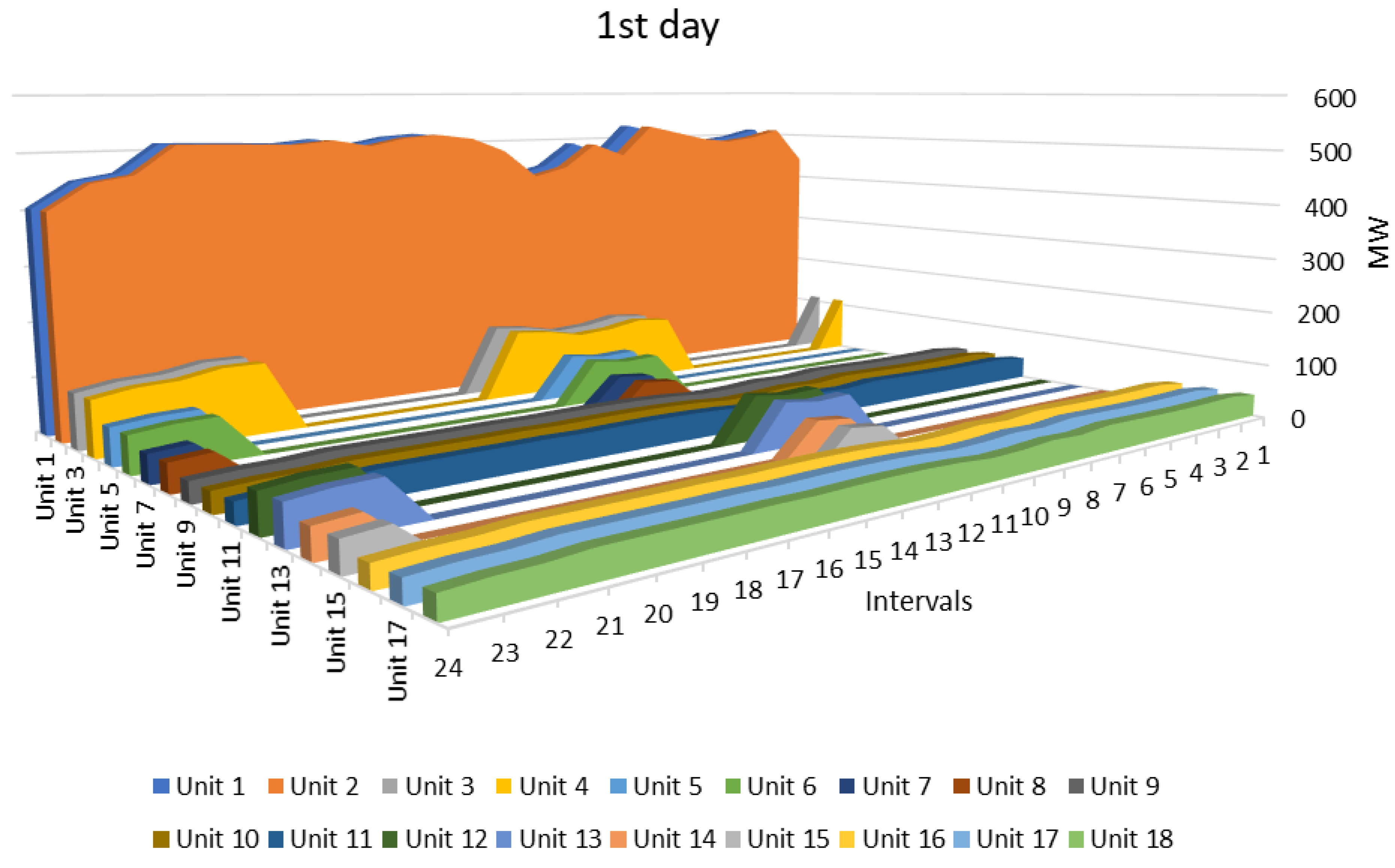
This corresponds to a TPC of 861.36 k$, obtained based on the following UC schedule (Figure 3).

Similar results were obtained by implementing simulations for the rest of the four weekdays. The performance is depicted in

Table 2. Results obtained through the conventional LR.

Assessed Weekday	Max (k)	ε	J (k$)
1	101	0.003	783.89
2	93	0.008	625.66
3	97	0.008	604.86
4	123	0.007	636.45
5	161	0.007	861.36

, where the number of iterations, the dual gap and the total production cost are included.

4.2. Comparison with Modern Insights

In this section, the most recent advances in the field of gradient-based optimization (GBO) and genetic algorithms are presented in order to evaluate and compare them with the proposed solution. Based on simulations obtained by applying the gradient-based optimization of [15], the TPC pertaining to the five-day optimal UC is rated at 2355.145 k$. The high production cost is formed by the increased number of committed generating units responding to the rapid changes in net load. Figure 4 justifies the obtained TPC, presenting the respective UC and power dispatch on the participating generating units.

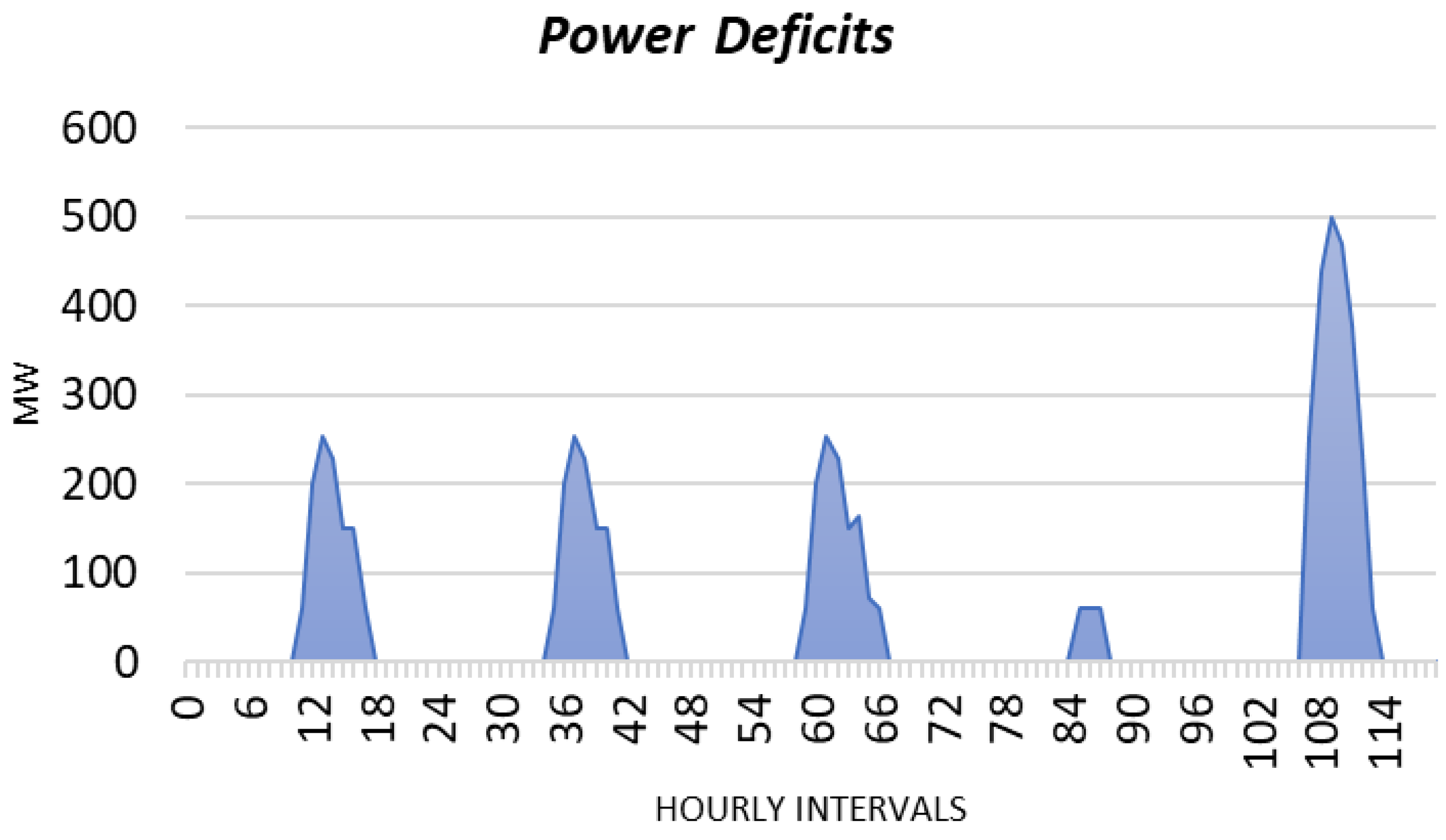
With respect to genetic algorithms, the available function GA in the MATLAB optimization toolbox was taken into account, considering two coupling constraints and mixed-integer limitations. The drawback of the developed algorithm lies in the increased number of function evaluations (showing an exponential increase compared with LR) and the violation of coupling constraints. As a result, a penalty cost for the P_ENS and P_SRNS retrieved as $\widehat{a}=max a_i, \widehat{b}=max b_i, \widehat{c}=max c_i$ was considered, resulting in a final TPC of 2378.296 k$. The power deficits can be seen in Figure 5.

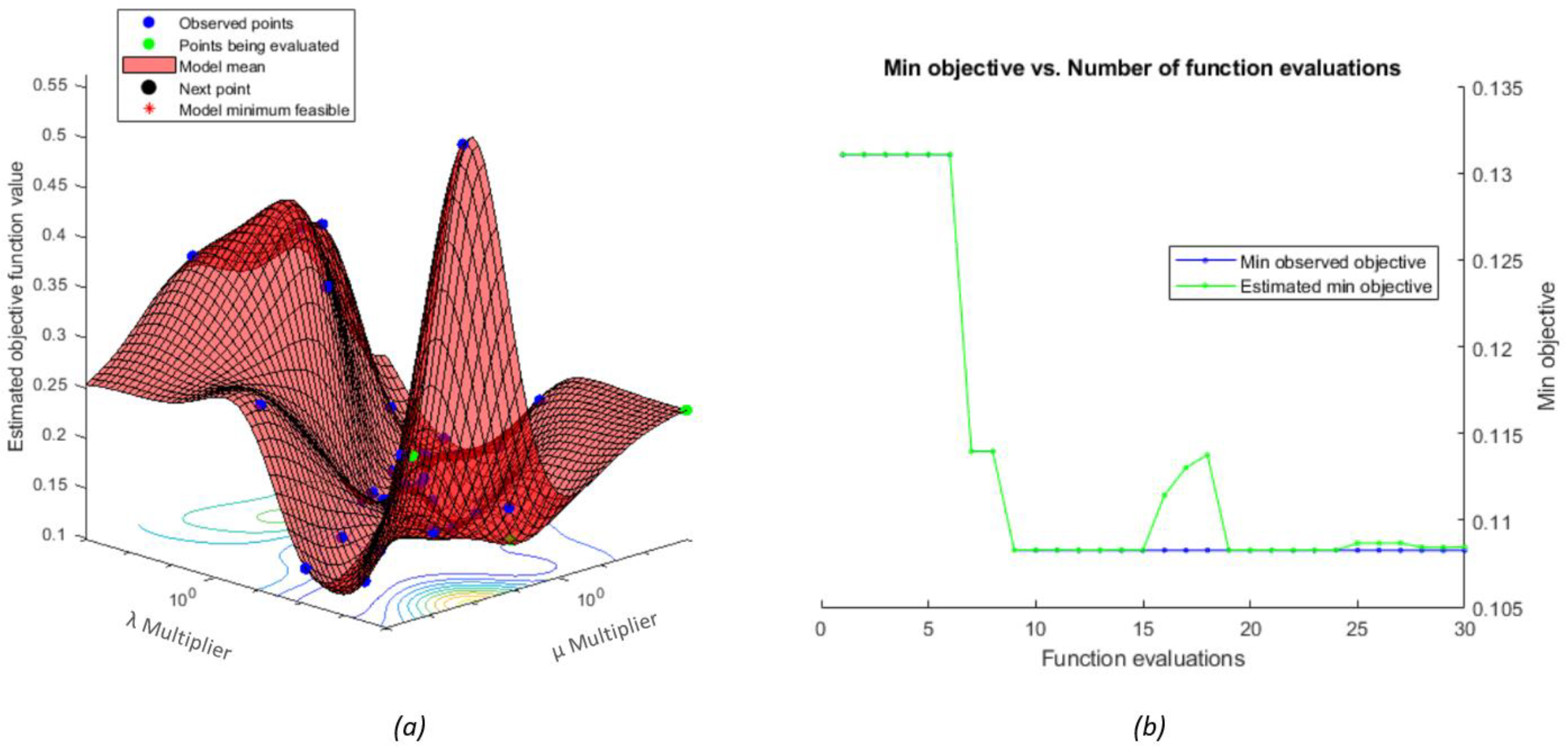
On the contrary, the variational Bayes alternative completely avoided oscillations based on a proper acquisition function. The employed acquisition function helps the optimization move toward regions with lower mean values (lowest cost) and maximum uncertainty (posterior variance) [37]. In this way, the procedure not only avoids trapping at local oscillations but also promises a guaranteed global solution, increasing the exploration space with the minimum number of function evaluations. In normalized values, the performance of the proposed approach during a certain time interval can be explained with the help of Figure 6. Figure 6a shows the estimated objective function across the Lagrange multipliers. The respective minimum TPC over the required function evaluations (iterations) is illustrated in Figure 6b. Assuming that the formulated coupling constraint of power balance is satisfied only when $\left(\sum S_i^t{P}_i^t-P_{net}^t-{10}^{-9}\right)\le 0$, its actual violation degree during an optimization loop can be expressed by Figure 7.

Applying simulations pertaining to the five weekdays, the optimal UC schedule greatly improved. Figure 8 presents the obtained contribution of the least committed units. The cumulative TPC achieved a drastic decrease in the order of −1.254 M$ (or a final of 2258.349 k$). The start-up cost, along with the fuel cost during each hourly interval, can be seen in Figure 9.

For the realization of the model developed based on variational Bayes, the settings utilized for control, initialization and stopping were the expected improvement acquisition function, 50% exploration ratio, 300-point Gaussian process fitness, four initial evaluation points, two non-deterministic coupling constraints and 30 maximum function evaluations without any initialization values for the optimizable variables, constraint violations or objective.

4.3. Prospects for Real-World Conditions

In real-world implementations, the RES contribution possesses the priority in the energy mix. Consequently, the penalty costs for the power not served from variable resources become superior in order to eliminate their curtailment. By enhancing the variable and uncertain resource penetration, the overall system inertia in terms of spinning reserve decreases, since the conventional generating units constitute the only source for the spinning reserve provision. An actual paradigm representing the residual load in contrast to the variable energy sources integration is depicted in Figure 10.

The actual values of the considered energy system pertaining to the worst day are tabulated in

Table 3. MW-output of different renewable systems across the residual load.

Interval	Biomass	Geothermal	PV	Wind	Hydro	Residual Load	SR
1	10	18	0	23	305	1458	45
2	10	18	0	2	296	1436	37
3	10	17	0	0	287	1395	35
4	10	17	0	0	283	1374	34
5	10	17	0	12	287	1384	39
6	10	18	0	4	296	1434	38
7	10	18	180	21	305	1279	58
8	10	19	200	2	322	1364	55
9	10	20	220	0	339	1431	58
10	10	22	220	1	374	1600	62
11	10	24	240	35	409	1716	81
12	10	27	312	351	461	1584	211
13	10	29	240	160	487	1975	137
14	10	30	220	152	496	2046	134
15	10	29	220	648	492	1528	320
16	10	28	200	279	479	1854	178
17	10	29	180	150	481	2013	128
18	10	28	0	121	466	2147	102
19	10	27	0	46	459	2189	73
20	10	27	0	277	452	1925	159
21	10	27	0	125	445	2044	101
22	10	23	0	96	394	1820	84
23	10	22	0	4	377	1833	47
24	10	20	0	0	334	1624	41

, along with the dynamic, spinning reserve requirement.

The sharp changes in the net load observed during periods with a high RES contribution require rapid-response generators to get online and follow the curve with minimum deviations. Apart from the increased ramping capability, these generators are usually expensive to start up, and in power systems with frequent renewable intermittency (e.g., due to unexpected cloud occurrences or steep wind gusts or falls), they may start up/shut down multiple times a day. On the contrary, the fuels used by rapid units with a high ramp capacity contribute less in terms of GHG emissions than they do in terms of energy consumption. They offer cleaner conversion with poor combustion indices [38].

Table 4. Emission features of the thermal generating units [39].

Unit i	e1 ($/MW2h)	e2 ($/MWh)	e3 ($/h)	SU Emission Cost ($)	Fuel Type
1	0.0022	0.478	7.712	743.84	Higher hydrocarbon
2	0.0022	0.478	7.712	743.84	Higher hydrocarbon
3	0.0022	0.478	7.712	743.84	Higher hydrocarbon
4	0.0022	0.478	7.712	743.84	Higher hydrocarbon
5	0.0022	0.478	7.712	743.84	Higher hydrocarbon
6	0.0022	0.478	7.712	743.84	Higher hydrocarbon
7	0.0022	0.478	7.712	743.84	Higher hydrocarbon
8	0.0022	0.478	7.712	743.84	Higher hydrocarbon
9	0.0018	0.438	1.317	85.36	Diesel
10	0.0018	0.438	1.317	85.36	Diesel
11	0.0018	0.438	1.317	85.36	Diesel
12	0.0022	0.478	7.712	743.84	Higher hydrocarbon
13	0.0022	0.478	7.712	743.84	Higher hydrocarbon
14	0.0022	0.478	7.712	743.84	Higher hydrocarbon
15	0.0022	0.478	7.712	743.84	Higher hydrocarbon
16	0.0018	0.438	1.317	743.84	Diesel
17	0.0018	0.438	1.317	85.36	Diesel
18	0.0018	0.438	1.317	85.36	Diesel

lists the CO₂ emission coefficients of the assessed generators in relation to their fuel type [29]. The indicated values account for 5$/tn of released CO₂ [37].

It is worth noting that expert systems and efficient algorithms are needed to handle the exploration–exploitation rates and, avoiding the local optima trapping, guide the optimization task towards global UC schedules with minimum TPC and maximum reliability. A realization of the problem based on the proposed approach is included in Figure 11.

5. Conclusions

In this work, a radically different approach to accelerating the Lagrangian multipliers towards optimal unit commitment has been presented. Based on the most recent advancements in variational Bayes, the conventional Lagrange relaxation technique has been enhanced to provide improved generation schedules during longer time-horizons at the least number of function evaluations. Formulating the complicating dual problem of unit commitment, an attempt was made in order to design a proper model that is able to lead optimization towards regions with minimum objective values and maximum uncertainty. In this way, the solutions cannot be trapped at the local minima but are driven to global solutions that undeniably improve the conventional mechanism that relied on simple dual decomposition. Utilizing the characteristics of 18 thermal generating units, the new approach compared well with its potential competitor under the same power system paradigm: a 120 h net-load demand. Based on the obtained results, the conventional Lagrange relaxation falls into oscillations which restrict the overall optimization task. As a result, to decrease the computational burden, smaller time horizons needed to take place (24 h load). Even in this case, the total production cost was too high in contrast to the overall cost obtained by making use of variational Bayes. This solution appears quite promising since it offers improved overall costs with less of a computational effort. Future works may regard the inclusion of renewable uncertainty in load and electricity storage.

References

1. Celasun, O.; Mineshima, A.; Arregui, N.; Mylonas, V.; Ari, A.; Teodoru, I.; Black, S.; Zhunussova, K.; Iakova, D.; Parry, I. Surging Energy Prices in Europe in the Aftermath of the War: How to Support the Vulnerable and Speed up the Transition Away from Fossil Fuels. IMF Work. Pap. 2022, 152, 1–41. Available online: https://ssrn.com/abstract=4184693 (accessed on 1 November 2022). [CrossRef]
2. Arias, A.F.; Lamadrid, A.; Valencia, C. Virtual Power Plant Day Ahead Energy Unit Commitment. In Proceedings of the 55th Hawaii International Conference on System Sciences, Maui, HI, USA, 4–7 January 2022; pp. 1–10. [Google Scholar] [CrossRef]
3. Feng, Z.-K.; Niu, W.-J.; Wang, W.-C.; Zhou, J.-Z.; Cheng, C.-T. A mixed integer linear programming model for unit commitment of thermal plants with peak shaving operation aspect in regional power grid lack of flexible hydropower energy. Energy 2019, 175, 618–629. [Google Scholar] [CrossRef]
4. Nikolaidis, P.; Poullikkas, A. Co-optimization of active power curtailment, load shedding and spinning reserve deficits through hybrid approach: Comparison of electrochemical storage technologies. IET Renew. Power Gener. 2022, 16, 92–104. [Google Scholar] [CrossRef]
5. Shahbazitabar, M.; Abdi, H. A novel priority-based stochastic unit commitment considering renewable energy sources and parking lot cooperation. Energy 2018, 161, 308–324. [Google Scholar] [CrossRef]
6. Colonetti, B.; Finardi, E.C. Combining Lagrangian relaxation, benders decomposition, and the level bundle method in the stochastic hydrothermal unit-commitment problem. Int. Trans. Electr. Energy Syst. 2020, 30, e12514. [Google Scholar] [CrossRef]
7. Shen, J.-J.; Shen, Q.-Q.; Cheng, C.-T.; Zhang, X.-F.; Wang, J. Large-Scale Unit Commitment for Cascaded Hydropower Plants with Hydraulic Coupling and Head-Sensitive Forbidden Zones: Case of the Xiluodu and Xiangjiaba Hydropower System. J. Water Resour. Plan. Manag. 2020, 146, 05020023. [Google Scholar] [CrossRef]
8. Scuzziato, M.R.; Finardi, E.C.; Frangioni, A. Solving stochastic hydrothermal unit commitment with a new primal recovery technique based on Lagrangian solutions. Int. J. Electr. Power Energy Syst. 2021, 127, 106661. [Google Scholar] [CrossRef]
9. Nikolaidis, P.; Poullikkas, A. Enhanced Lagrange relaxation for the optimal unit commitment of identical generating units. IET Gener. Transm. Distrib. 2020, 14, 3920–3928. [Google Scholar] [CrossRef]
10. Ponciroli, R.; Stauff, N.E.; Ramsey, J.; Ganda, F.; Vilim, R.B. An improved genetic algorithm approach to the unit commitment/economic dispatch problem. IEEE Trans. Power Syst. 2020, 35, 4005–4013. [Google Scholar] [CrossRef]
11. Jordehi, A.R. An improved particle swarm optimisation for unit commitment in microgrids with battery energy storage systems considering battery degradation and uncertainties. Int. J. Energy Res. 2021, 45, 727–744. [Google Scholar] [CrossRef]
12. Garlík, B.; Křivan, M. Renewable energy unit commitment, with different acceptance of balanced power, solved by simulated annealing. Energy Build. 2013, 67, 392–402. [Google Scholar] [CrossRef]
13. Columbus, C.C.; Chandrasekaran, K.; Simon, S.P. Nodal ant colony optimization for solving profit based unit commitment problem for GENCOs. Appl. Soft Comput. J. 2012, 12, 145–160. [Google Scholar] [CrossRef]
14. Sudhakaran, M.; Raj, P. Integrating genetic algorithms and tabu search for unit commitment problem. Int. J. Eng. Sci. Technol. 2010, 2, 57–69. [Google Scholar] [CrossRef]
15. Said, M.; Houssein, E.H.; Deb, S.; Alhussan, A.A.; Ghoniem, R.M. A Novel Gradient Based Optimizer for Solving Unit Commitment Problem. IEEE Access 2022, 10, 18081–18092. [Google Scholar] [CrossRef]
16. Srikanth, K.; Panwar, L.K.; Panigrahi, B.; Herrera-Viedma, E.; Sangaiah, A.K.; Wang, G.-G. Meta-heuristic framework: Quantum inspired binary grey wolf optimizer for unit commitment problem. Comput. Electr. Eng. 2018, 70, 243–260. [Google Scholar] [CrossRef]
17. Yang, K.; Yang, K. Short-Term Hydro Generation Scheduling of the Three Gorges Hydropower Station Using Improver Binary-coded Whale Optimization Algorithm. Water Resour. Manag. 2021, 35, 3771–3790. [Google Scholar] [CrossRef]
18. Anand, H.; Narang, N.; Dhillon, J. Profit based unit commitment using hybrid optimization technique. Energy 2018, 148, 701–715. [Google Scholar] [CrossRef]
19. Pan, J.-S.; Hu, P.; Chu, S.-C. Binary fish migration optimization for solving unit commitment. Energy 2021, 226, 120329. [Google Scholar] [CrossRef]
20. Zhao, J.; Liu, S.; Zhou, M.; Guo, X.; Qi, L. An Improved Binary Cuckoo Search Algorithm for Solving Unit Commitment Problems: Methodological Description. IEEE Access 2018, 6, 43535–43545. [Google Scholar] [CrossRef]
21. Dhaliwal, J.S.; Dhillon, J. Profit based unit commitment using memetic binary differential evolution algorithm. Appl. Soft Comput. J. 2019, 81, 105502. [Google Scholar] [CrossRef]
22. Reddy, S.; Panwar, L.K.; Panigrahi, B.K.; Kumar, R. Solution to unit commitment in power system operation planning using binary coded modified moth flame optimization algorithm (BMMFOA): A flame selection based computational technique. J. Comput. Sci. 2018, 25, 298–317. [Google Scholar] [CrossRef]
23. Ali, E.; Elazim, S.A.; Balobaid, A. Implementation of coyote optimization algorithm for solving unit commitment problem in power systems. Energy 2023, 263, 125697. [Google Scholar] [CrossRef]
24. Kumar, V.; Naresh, R. Application of baron solver for solution of cost based unit commitment problem. Int. J. Electr. Eng. Inform. 2020, 12, 807–827. [Google Scholar] [CrossRef]
25. Amudha, A.; Varghese, M.P. A Hybrid CS-ABC optimization technique for Solving Unit Commitment Problem with Wind Power Uncertainty. Appl. Math. Inf. Sci. 2019, 13, 417–429. [Google Scholar] [CrossRef]
26. Singh, V.; Fozdar, M.; Malik, H.; Márquez, F.P.G. Transmission congestion management through sensitivity based rescheduling of generators using improved monarch butterfly optimization. Int. J. Electr. Power Energy Syst. 2023, 145, 108729. [Google Scholar] [CrossRef]
27. Nandi, A.; Kamboj, V.K.; Khatri, M. Metaheuristics approaches to profit based unit commitment for GENCOs. Mater. Today Proc. 2022, 60, 1874–1881. [Google Scholar] [CrossRef]
28. Mrówczyńska, M.; Skiba, M.; Leśniak, A.; Bazan-Krzywoszańska, A.; Janowiec, F.; Sztubecka, M.; Grech, R.; Kazak, J. A new fuzzy model of multi-criteria decision support based on Bayesian networks for the urban areas’ decarbonization planning. Energy Convers. Manag. 2022, 268, 116035. [Google Scholar] [CrossRef]
29. Nikolaidis, P.; Poullikkas, A. A Thorough Emission-Cost Analysis of the Gradual Replacement of Carbon-Rich Fuels with Carbon-Free Energy Carriers in Modern Power Plants: The Case of Cyprus. Sustainability 2022, 14, 10800. [Google Scholar] [CrossRef]
30. Nikolaidis, P.; Poullikkas, A. A novel cluster-based spinning reserve dynamic model for wind and PV power reinforcement. Energy 2021, 234, 121270. [Google Scholar] [CrossRef]
31. Nikolaidis, P.; Poullikkas, A. Evolutionary Priority-Based Dynamic Programming for the Adaptive Integration of Intermittent Distributed Energy Resources in Low-Inertia Power Systems. Eng 2021, 2, 643–660. [Google Scholar] [CrossRef]
32. Cheng, C.-P.; Liu, C.-W.; Liu, C.-C. Unit commitment by Lagrangian Relaxation and Genetic Algorithms. IEEE Trans. Power Syst. 2000, 15, 707–714. [Google Scholar] [CrossRef]
33. Rush, A.M.; Collins, M.J. A tutorial on dual decomposition and lagrangian relaxation for inference in natural language processing. J. Artif. Intell. Res. 2012, 45, 305–362. [Google Scholar] [CrossRef]
34. Nikolaidis, P.; Antoniades, A.; Chatzis, S. A bayesian optimization approach for the robust unit commitment of identical generating units. In Proceedings of the 12th Mediterranean Conference on Power Generation, Transmission, Distribution and Energy Conversion (MEDPOWER 2020), Online, 9–12 November 2020; pp. 264–269. [Google Scholar]
35. Hernández-Lobato, J.M.; Gelbart, M.A.; Adams, R.P.; Hoffman, M.W.; Ghahramani, Z. A general framework for constrained Bayesian optimization using information-based search. J. Mach. Learn. Res. 2016, 17, 1–53. [Google Scholar]
36. Jordan, L.K.; Ghahramani, M.I.; Jaakkola, Z.; Saul, T.S. An Introduction to Variational Methods for Graphical Models. Mach. Learn. 1999, 37, 183–233. [Google Scholar] [CrossRef]
37. Nikolaidis, P.; Chatzis, S. Gaussian process-based Bayesian optimization for data-driven unit commitment. Int. J. Electr. Power Energy Syst. 2021, 130, 106930. [Google Scholar] [CrossRef]
38. Fritt-Rasmussen, J.; Wegeberg, S.; Gustavson, K.; Sørheim, K.R.; Daling, P.S.; Jørgensen, K.; Tonteri, O.; Holst-Andersen, J.P. Heavy Fuel Oil (HFO): A Review of Fate and Behaviour of HFO Spills in Cold; Nordic Council of Ministers: Copenhagen, Denmark, 2018. [Google Scholar] [CrossRef]
39. Nikolaidis, P.; Poullikkas, A. Optimal carbon-electricity trade-offs through the virtual power plant concept. Discov. Energy 2022, 2, 1–16. [Google Scholar] [CrossRef]
Figure 1. Net-load demand (MW) for 120 weekday hours.
Algorithms 16 00020 g001
Figure 2. Performance of the conventional LR approach during the first 24 h residual demand.
Algorithms 16 00020 g002
Figure 3. Optimal UC schedule via the LR approach pertaining to the first 24 h residual demand.
Algorithms 16 00020 g003
Figure 4. Performance of the gradient-based optimization pertaining to the five-day paradigm.
Algorithms 16 00020 g004
Figure 5. Power deficits applying the genetic algorithm mechanism.
Algorithms 16 00020 g005
Figure 6. Estimated minimum objective function value across (a) the Lagrange multipliers and (b) the required function evaluations.
Algorithms 16 00020 g006
Figure 7. Power-balance violation degree during a variational Bayes optimization loop.
Algorithms 16 00020 g007
Figure 8. Optimal UC through the novel variational Bayes approach.
Algorithms 16 00020 g008
Figure 9. Start-up versus total production cost with the variational Bayes paradigm.
Algorithms 16 00020 g009
Figure 10. Residual load and renewable energy contribution during the examined period.
Algorithms 16 00020 g010
Figure 11. Optimal UC schedule obtained by the proposed approach in a real-world scenario.
Algorithms 16 00020 g011