


Classification of Program Texts Represented as Markov Chains with Biology-Inspired Algorithms-Enhanced Extreme Learning Machines


Abstract
:1. Introduction
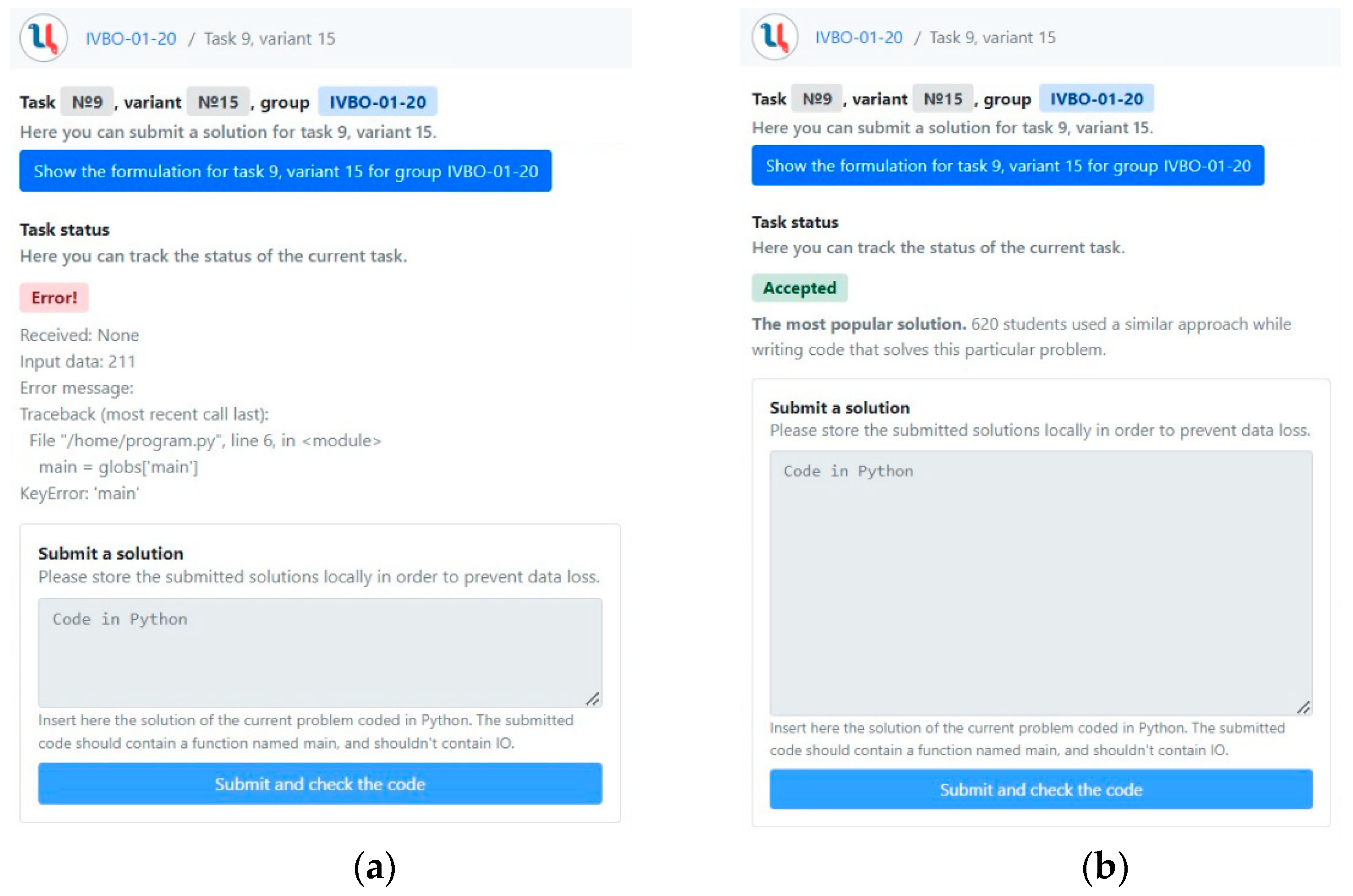
2. Digital Teaching Assistant
3. Program Text Vectorization
| Algorithm 1 Vectorization of a set of program texts based on Markov chains. | |
| Input: | -a set containing program texts. |
| 1. | Define the set of Markov chain state transition graphs . |
| 2. | Define {Import, Load, Store, alias, arguments, arg, Module, keyword}. |
| 3. | For each program text do: |
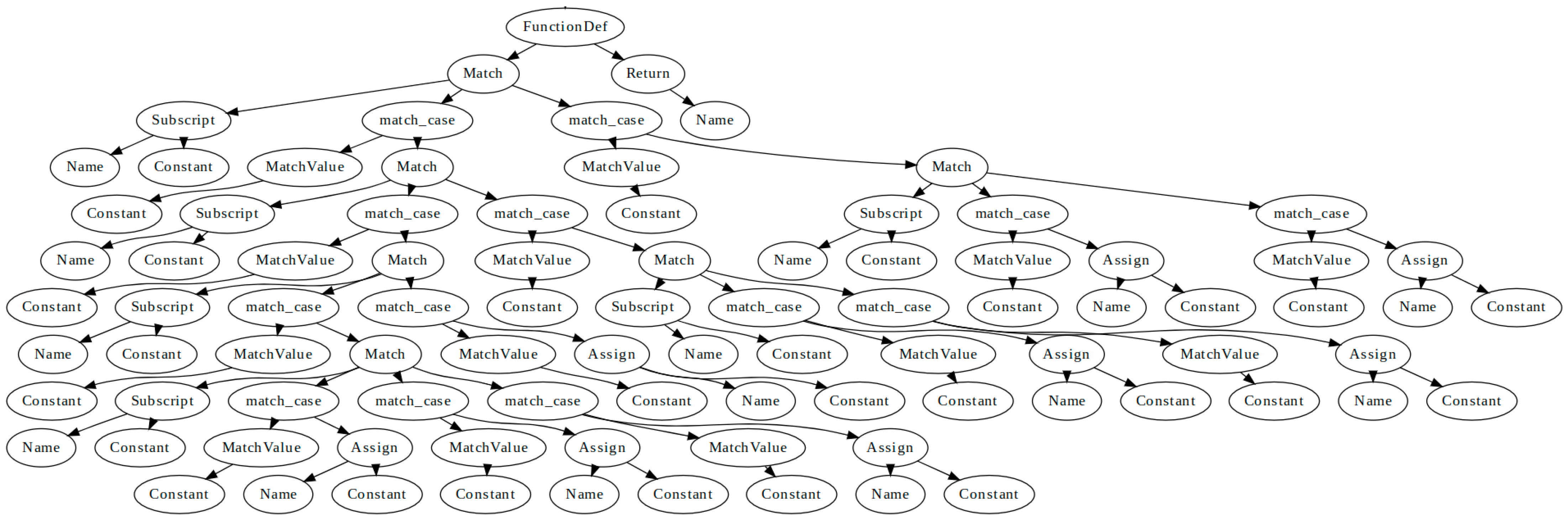
| 4. | Construct an AST for using Python standard library (see Figure 2). |
| 5. | Remove nodes belonging to the set from . |
| 6. | Replace nodes in according to Table 2. |
| 7. | Construct Markov chain state transition graph for (see Figure 3). |
| 8. | . |
| 9. | End loop. |
| 10. | Define the set with all different node types existing in graphs from . |
| 11. | Define the set of vector representations of program texts . |
| 12. | For each Markov chain state transition graph do: |
| 13. | Construct an adjacency matrix for the weighted graph . |
| 14. | Reshape the matrix to vector , where . |
| 15. | . |
| 16. | End loop. |
| 17. | Return the set of vector representations of program texts and the set . |
| Algorithm 2 Vectorization of a single program text based on Markov chains. | |
| Input: | -a program text, -a set with all different node types that exist in Markov chains of programs solving tasks of the same type as , this set is obtained by Algorithm 1. |
| 1. | Define {Import, Load, Store, alias, arguments, arg, Module, keyword}. |
| 2. | Construct an AST for using Python standard library (see Figure 2). |
| 3. | Remove nodes belonging to the set from . |
| 4. | Replace nodes in according to Table 2. |
| 5. | Construct Markov chain state transition graph for (see Figure 3). |
| 6. | Construct an adjacency matrix for the weighted graph . |
| 7. | Reshape the matrix to vector , where . |
| 8. | Return the vector representing the program text. |
4. Program Text Classification
4.1. Support Vector Machine Classifier
4.2. K Nearest Neighbors Classifier
4.3. Random Forest Classifier
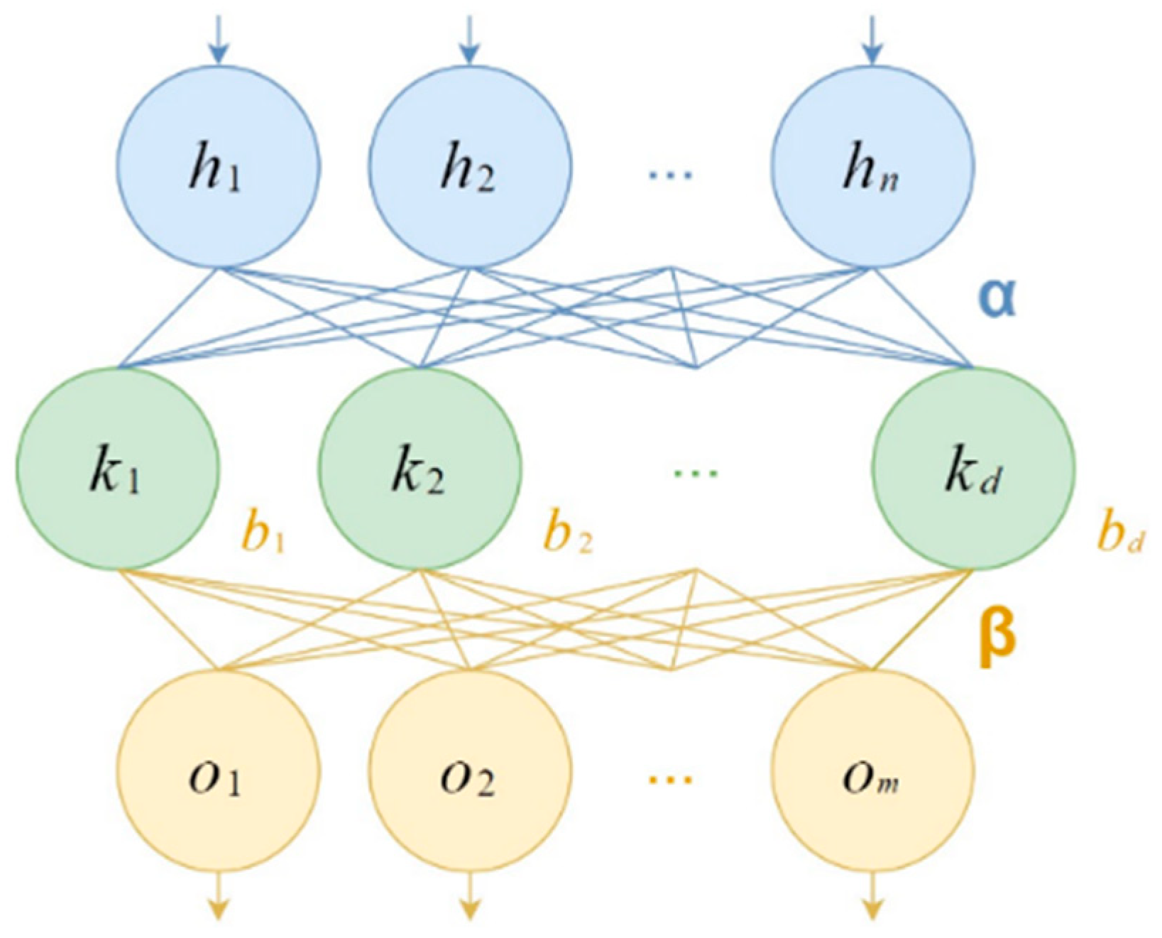
4.4. Extreme Learning Machine Classifier
| Algorithm 3 Extreme learning machine training. | |
| Input: | -matrix of rows encoding -dimensional input vectors, -matrix of rows encoding -dimensional output vectors, -regularization parameter, -hidden neuron count, -hidden layer activation function. |
| 1. | Initialize the weights with uniformly distributed random numbers. |
| 2. | Initialize the biases with uniformly distributed random numbers. |
| 3. | Compute by cloning times. |
| 4. | Compute hidden layer output matrix . |
| 5. | Initialize the identity matrix . |
| 6. | Compute pseudoinverse . |
| 7. | Compute the weights according to . |
| 8. | Return input weights , biases , output weights . |
| Algorithm 4 Extreme learning machine predictions. | |
| Input: | -matrix of rows encoding -dimensional input vectors, -regularization parameter, -hidden neuron count, -hidden layer activation function, -input weights, -hidden layer biases, -output weights. |
| 1. | Compute by cloning times. |
| 2. | Compute hidden layer output matrix . |
| 3. | Compute the output matrix belonging to . |
| 4. | Return the matrix of rows encoding -dimensional output vectors. |
4.5. Multi-Class Classification Metrics
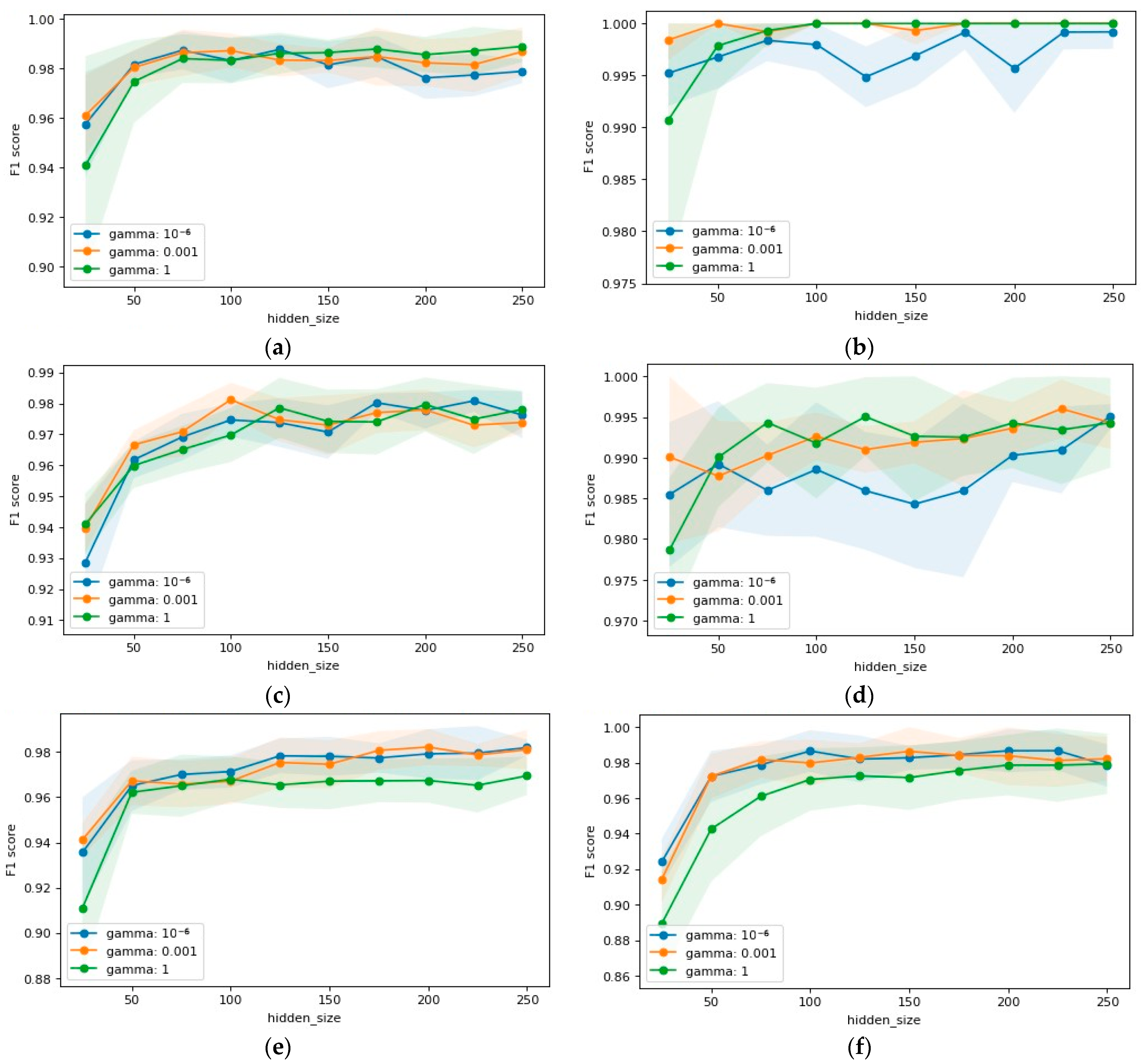
4.6. Biology-Inspired Algorithms-Enhanced Extreme Learning Machines
5. Numerical Experiment
6. Discussion
Author Contributions
Funding
Data Availability Statement
Conflicts of Interest
References
- Moussiades, L.; Vakali, A. PDetect: A clustering approach for detecting plagiarism in source code datasets. Comput. J. 2005, 48, 651–661. [Google Scholar] [CrossRef]
- Kustanto, C.; Liem, I. Automatic Source Code Plagiarism Detection. In Proceedings of the 2009 10th ACIS International Conference on Software Engineering, Artificial Intelligences, Networking and Parallel/Distributed Computing, Daegu, Korea, 27–29 May 2009; IEEE: Pistacaway, NJ, USA, 2009; pp. 481–486. [Google Scholar]
- Jiang, L.; Misherghi, G.; Su, Z.; Glondu, S. Deckard: Scalable and Accurate Tree-Based Detection of Code Clones. In Proceedings of the 29-th International Conference on Software Engineering (ICSE’07), Minneapolis, MN, USA, 20–26 May 2007; IEEE: Pistacaway, NJ, USA, 2007; pp. 96–105. [Google Scholar]
- Chilowicz, M.; Duris, E.; Roussel, G. Syntax Tree Fingerprinting for Source Code Similarity Detection. In Proceedings of the 2009 IEEE 17th International Conference on Program Comprehension, Vancouver, BC, Canada, 17–19 May 2009; IEEE: Pistacaway, NJ, USA, 2009; pp. 243–247. [Google Scholar]
- Yasaswi, J.; Kailash, S.; Chilupuri, A.; Purini, S.; Jawahar, C.V. Unsupervised Learning-Based Approach for Plagiarism Detection in Programming Assignments. In Proceedings of the 10th Innovations in Software Engineering Conference, Jaipur, India, 5–7 February 2017; Association for Computing Machinery: New York, NY, USA, 2017; pp. 117–121. [Google Scholar]
- Sovietov, P. Automatic Generation of Programming Exercises. In Proceedings of the 2021 1st International Conference on Technology Enhanced Learning in Higher Education (TELE), Lipetsk, Russia, 24–25 June 2021; IEEE: Pistacaway, NJ, USA, 2021; pp. 111–114. [Google Scholar]
- Wakatani, A.; Maeda, T. Automatic Generation of Programming Exercises for Learning Programming Language. In Proceedings of the 2015 IEEE/ACIS 14th International Conference on Computer and Information Science (ICIS), Las Vegas, NV, USA, 28 June–1 July 2015; IEEE: Pistacaway, NJ, USA, 2015; pp. 461–465. [Google Scholar]
- Staubitz, T.; Klement, H.; Renz, J.; Teusner, R.; Meinel, C. Towards Practical Programming Exercises and Automated Assessment in Massive Open Online Courses. In Proceedings of the 2015 IEEE International Conference on Teaching, Assessment, and Learning for Engineering (TALE), Zhuhai, China, 10–12 December 2015; IEEE: Pistacaway, NJ, USA, 2015; pp. 23–30. [Google Scholar]
- Sovietov, P.N.; Gorchakov, A.V. Digital Teaching Assistant for the Python Programming Course. In Proceedings of the 2022 2nd International Conference on Technology Enhanced Learning in Higher Education (TELE), Lipetsk, Russia, 26–27 May 2022; IEEE: Pistacaway, NJ, USA, 2022; pp. 272–276. [Google Scholar]
- Andrianova, E.G.; Demidova, L.A.; Sovetov, P.N. Pedagogical design of a digital teaching assistant in massive professional training for the digital economy. Russ. Technol. J. 2022, 10, 7–23. [Google Scholar] [CrossRef]
- Su, C.H.; Cheng, C.H. A mobile gamification learning system for improving the learning motivation and achievements. J. Comput. Assist. Learn. 2015, 31, 268–286. [Google Scholar] [CrossRef]
- Cortes, C.; Vapnik, V. Support-vector Networks. Mach. Learn. 1995, 20, 273–297. [Google Scholar] [CrossRef]
- Altman, N.S. An introduction to kernel and nearest-neighbor nonparametric regression. Am. Stat. 1992, 46, 175–185. [Google Scholar]
- Wu, Y.; Ianakiev, K.; Govindaraju, V. Improved K-nearest neighbor classification. Pattern Recognit. 2002, 35, 2311–2318. [Google Scholar] [CrossRef]
- Ho, T.K. Random Decision Forests. In Proceedings of the 3rd International Conference on Document Analysis and Recognition, Montreal, QC, Canada, 14–16 August 1995; IEEE: Pistacaway, NJ, USA, 1995; pp. 278–282. [Google Scholar]
- Rosenblatt, F. The perceptron: A probabilistic model for information storage and organization in the brain. Psychol. Rev. 1958, 65, 386–408. [Google Scholar] [CrossRef]
- Ruder, S. An overview of gradient descent optimization algorithms. arXiv 2016, arXiv:1609.04747. [Google Scholar]
- Chen, N.; Xiong, C.; Du, W.; Wang, C.; Lin, X.; Chen, Z. An improved genetic algorithm coupling a back-propagation neural network model (IGA-BPNN) for water-level predictions. Water 2019, 11, 1795. [Google Scholar] [CrossRef]
- Demidova, L.A.; Gorchakov, A.V. A Study of Biology-inspired Algorithms Applied to Long Short-Term Memory Network Training for Time Series Forecasting. In Proceedings of the 2021 3rd International Conference on Control Systems, Mathematical Modeling, Automation and Energy Efficiency (SUMMA), Lipetsk, Russia, 10–12 November 2021; IEEE: Pistacaway, NJ, USA, 2021; pp. 473–478. [Google Scholar]
- Huang, G.B.; Zhu, Q.Y.; Siew, C.K. Extreme Learning machine: Theory and applications. Neurocomputing 2006, 70, 489–501. [Google Scholar] [CrossRef]
- Rao, C.R. Generalized Inverse of a Matrix and its Applications. In Proceedings of the Sixth Berkeley Symposium on Mathematical Statistics and Probability, Theory of Statistics, Berkeley, CA, USA, 21 June–18 July 1970; University of California Press: Berkeley, CA, USA, 1972; pp. 601–620. [Google Scholar]
- Cheng, C.; Tay, W.P.; Huang, G.B. Extreme Learning Machines for Intrusion Detection. In Proceedings of the 2012 International Joint Conference on Neural Networks (IJCNN), Brisbane, Australia, 10–15 June 2012; IEEE: Pistacaway, NJ, USA, 2012; pp. 1–8. [Google Scholar]
- Liu, Y.; Loh, H.T.; Tor, S.B. Comparison of Extreme Learning Machine with Support Vector Machine for Text Classification. In Proceedings of the International Conference on Industrial, Engineering and Other Applications of Applied Intelligent Systems, Innovations in Applied Artificial Intelligence, Bari, Italy, 22–24 June 2005; Springer: Berlin, Germany, 2005; pp. 390–399. [Google Scholar]
- Demidova, L.A.; Gorchakov, A.V. Application of bioinspired global optimization algorithms to the improvement of the prediction accuracy of compact extreme learning machines. Russ. Technol. J. 2022, 10, 59–74. [Google Scholar] [CrossRef]
- Cai, W.; Yang, J.; Yu, Y.; Song, Y.; Zhou, T.; Qin, J. PSO-ELM: A hybrid learning model for short-term traffic flow forecasting. IEEE Access 2020, 8, 6505–6514. [Google Scholar] [CrossRef]
- Song, S.; Wang, Y.; Lin, X.; Huang, Q. Study on GA-based Training Algorithm for Extreme Learning Machine. In Proceedings of the 2015 7th International Conference on Intelligent Human-Machine Systems and Cybernetics, Hangzhou, China, 26–27 August 2015; IEEE: Pistacaway, NJ, USA, 2015; Volume 2, pp. 132–135. [Google Scholar]
- Eremeev, A.V. A genetic algorithm with tournament selection as a local search method. J. Appl. Ind. Math 2012, 6, 286–294. [Google Scholar] [CrossRef]
- Kennedy, J.; Eberhart, R. Particle swarm optimization. In Proceedings of the ICNN’95-International Conference on Neural Networks, Perth, WA, Australia, 27 November–1 December 1995; Volume 4, pp. 1942–1948. [Google Scholar]
- Storn, R.; Price, K. Differential evolution—A simple and efficient heuristic for global optimization over continuous spaces. J. Glob. Optim. 1997, 11, 341–359. [Google Scholar] [CrossRef]
- Monteiro, R.P.; Verçosa, L.F.V.; Bastos-Filho, C.J.A. Improving the performance of the fish school search algorithm. Int. J. Swarm Intell. Res. 2018, 9, 21–46. [Google Scholar] [CrossRef]
- Stanovov, V.; Akhmedova, S.; Semenkin, E. Neuroevolution of augmented topologies with difference-based mutation. IOP Conf. Ser. Mater. Sci. Eng. 2021, 1047, 012075. [Google Scholar] [CrossRef]
- Ananthi, J.; Ranganathan, V.; Sowmya, B. Structure Optimization Using Bee and Fish School Algorithm for Mobility Prediction. Middle-East J. Sci. Res 2016, 24, 229–235. [Google Scholar]
- Prosvirin, A.; Duong, B.P.; Kim, J.M. SVM Hyperparameter Optimization Using a Genetic Algorithm for Rub-Impact Fault Diagnosis. Adv. Comput. Commun. Comput. Sci. 2019, 924, 155–165. [Google Scholar]
- Baioletti, M.; Di Bari, G.; Milani, A.; Poggioni, V. Differential Evolution for Neural Networks Optimization. Mathematics 2020, 8, 69. [Google Scholar] [CrossRef]
- Gilda, S. Source Code Classification using Neural Networks. In Proceedings of the 2017 14th International Joint Conference on Computer Science and Software Engineering (JCSSE), Nakhon Si Thammarat, Thailand, 12–14 July 2017; IEEE: Pistacaway, NJ, USA, 2017; pp. 1–6. [Google Scholar]
- Alon, U.; Zilberstein, M.; Levy, O.; Yahav, E. code2vec: Learning Distributed Representations of Code. In Proceedings of the ACM on Programming Languages, Athens, Greece, 21–22 October 2019; Association for Computing Machinery: New York, NY, USA, 2019; Volume 3, pp. 1–29. [Google Scholar]
- Gansner, E.R.; North, S.C. An Open Graph Visualization System and Its Applications to Software Engineering. Softw. Pract. Exp. 2000, 30, 1203–1233. [Google Scholar] [CrossRef]
- Berthiaux, H.; Mizonov, V. Applications of Markov chains in particulate process engineering: A review. Can. J. Chem. Eng. 2004, 82, 1143–1168. [Google Scholar] [CrossRef]
- Pedregosa, F.; Varoquaux, G.; Gramfort, A.; Michel, V.; Thirion, B.; Grisel, O.; Blondel, M.; Prettenhofer, P.; Weiss, R.; Dubourg, V.; et al. Scikit-learn: Machine learning in Python. J. Mach. Learn. Res. 2011, 12, 2825–2830. [Google Scholar]
- Harris, C.R.; Millman, K.J.; van der Walt, S.J.; Gommers, R.; Virtanen, P.; Cournapeau, D.; Wieser, E.; Taylor, J.; Berg, S.; Smith, N.J.; et al. Array programming with NumPy. Nature 2020, 585, 357–362. [Google Scholar] [CrossRef] [PubMed]
- Hsu, C.-W.; Lin, C.-J. A comparison of methods for multiclass support vector machines. IEEE Trans. Neural Netw. 2002, 13, 415–425. [Google Scholar]
- Parmar, A.; Katariya, R.; Patel, V. A Review on Random Forest: An Ensemble Classifier. In Proceedings of the International Conference on Intelligent Data Communication Technologies and Internet of Things, Coimbatore, India, 7–8 August 2018; Springer: Cham, Switzerland, 2018; pp. 758–763. [Google Scholar]
- Schmidt, W.F.; Kraaijveld, M.A.; Duin, R.P. W Feedforward Neural Networks with Random Weights. In Proceedings of the 11th IAPR International Conference on Pattern Recognition, Pattern Recognition Methodology and Systems, The Hague, The Netherlands, 30 August–3 September 1992; IEEE: Pistacaway, NJ, USA, 1992; Volume 2, pp. 1–4. [Google Scholar]
- Pao, Y.H.; Takefji, Y. Functional-link net computing: Theory, system architecture, and functionalities. Computer 1992, 25, 76–79. [Google Scholar] [CrossRef]
- Cao, W.; Gao, J.; Ming, Z.; Cai, S. Some tricks in parameter selection for extreme learning machine. IOP Conf. Ser. Mater. Sci. Eng. 2017, 261, 012002. [Google Scholar] [CrossRef]
- Grandini, M.; Bagli, E.; Visani, G. Metrics for Multi-class Classification: An Overview. arXiv 2020, arXiv:2008.05756. [Google Scholar]
- Demidova, L.A. Two-Stage Hybrid Data Classifiers Based on SVM and kNN Algorithms. Symmetry 2021, 13, 615. [Google Scholar] [CrossRef]
- Liu, G.; Zhao, H.; Fan, F.; Liu, G.; Xu, Q.; Nazir, S. An Enhanced Intrusion Detection Model Based on Improved kNN in WSNs. Sensors 2022, 22, 1407. [Google Scholar] [CrossRef]
- Razaque, A.; Ben Haj Frej, M.; Almi’ani, M.; Alotaibi, M.; Alotaibi, B. Improved Support Vector Machine Enabled Radial Basis Function and Linear Variants for Remote Sensing Image Classification. Sensors 2021, 21, 4431. [Google Scholar] [CrossRef]
- Demidova, L.A.; Gorchakov, A.V. A Study of Chaotic Maps Producing Symmetric Distributions in the Fish School Search Optimization Algorithm with Exponential Step Decay. Symmetry 2020, 12, 784. [Google Scholar] [CrossRef]
- Tapson, J.; Chazal, P.D.; Schaik, A.V. Explicit Computation of Input Weights in Extreme Learning Machines. In Proceedings of the ELM-2014, Singapore, 8–10 December 2014; Springer: Cham, Switzerland, 2014; Volume 1, pp. 41–49. [Google Scholar]
- Cao, Z.; Chu, Z.; Liu, D.; Chen, Y. A Vector-Based Representation to Enhance Head Pose Estimation. In Proceedings of the IEEE/CVF Winter Conference on Applications of Computer Vision, Hawaii, HI, USA, 19–25 June 2021; IEEE: Pistacaway, NJ, USA, 2021; pp. 1188–1197. [Google Scholar]
- Wang, Q.; Fang, Y.; Ravula, A.; Feng, F.; Quan, X.; Liu, D. WebFormer: The Web-Page Transformer for Structure Information Extraction. In Proceedings of the ACM Web Conference 2022, Lyon, France, 25–29 April 2022; Association for Computing Machinery: New York, NY, USA, 2022; pp. 3124–3133. [Google Scholar]


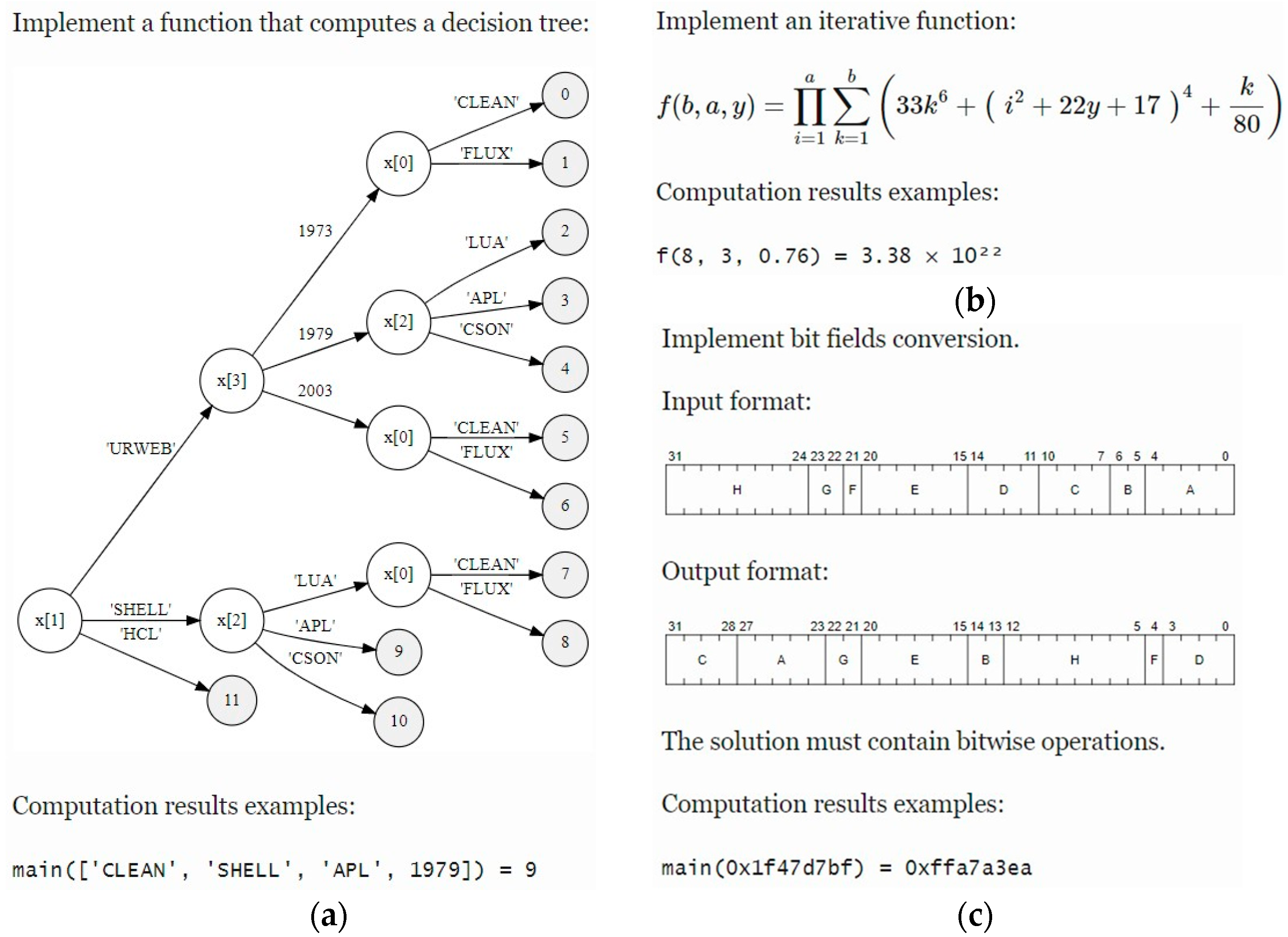
| Task Type | Brief Description |
|---|---|
| 1 | Implement a function |
| 2 | Implement a piecewise function |
| 3 | Implement an iterative function |
| 4 | Implement a recurrent function |
| 5 | Implement a function that operates on vectors |
| 6 | Implement a function that computes a decision tree |
| 7 | Implement bit fields conversion |
| 8 | Implement text format parsing |
| 9 | Implement a Mealy finite-state machine |
| 10 | Implement tabular data transformation |
| 11 | Implement binary data format parsing |
| Replacements for 1–11 Task Types | Replacements for 6–11 Task Types | ||
|---|---|---|---|
| Replaceable Vertex | Replacement | Replaceable Vertex | Replacement |
| Constant, Attribute | Name | List, Tuple, Set | List |
| BoolOp, Call, UnaryOp, BinOp | Op | Lambda, JoinedStr, FormattedValue | Name |
| Lt, LtE | Less | Pass, Break, Continue | None |
| Gt, GtE | Greater | ExceptHandler | Try |
| AugAssign, AnAssign | Assign | IfExp | If |
| match_case, MatchStar, MatchAs, MatchOr, MatchSingleton, MatchSequence, MatchMapping, MatchClass | MatchValue | For, While, ListComp, SetComp, DictComp, GeneratorExp, comprehension | Loop |
| UAdd | Add | ||
| USub | Sub | ||
| Task Type | Training Dataset Size | Testing Dataset Size | Class Count |
|---|---|---|---|
| 1 | 918 | 394 | 4 |
| 2 | 903 | 387 | 4 |
| 3 | 847 | 364 | 3 |
| 4 | 830 | 356 | 5 |
| 5 | 863 | 370 | 5 |
| 6 | 862 | 370 | 8 |
| 7 | 871 | 374 | 6 |
| 8 | 860 | 369 | 5 |
| 9 | 861 | 370 | 8 |
| 10 | 847 | 364 | 5 |
| 11 | 821 | 353 | 14 |
| Task Type | RF | SVM | KNN | ELM | ||||
|---|---|---|---|---|---|---|---|---|
| Depth | Trees | C | Kernel | K | Weights | Neurons | ||
| 1 | 10 | 40 | 1 | Linear | 3 | Uniform | 10−6 | 25 |
| 2 | 20 | 120 | 10 | RBF | 3 | Uniform | 0.001 | 125 |
| 3 | 10 | 100 | 1 | RBF | 3 | Uniform | 10−6 | 150 |
| 4 | 10 | 100 | 1 | Linear | 3 | Uniform | 10−6 | 75 |
| 5 | 20 | 100 | 1 | Linear | 3 | Uniform | 10−6 | 25 |
| 6 | 10 | 80 | 25 | Sigmoid | 3 | Distance | 1 | 250 |
| 7 | 20 | 60 | 1 | Linear | 8 | Uniform | 0.001 | 50 |
| 8 | 20 | 120 | 20 | RBF | 4 | Distance | 0.001 | 100 |
| 9 | 20 | 60 | 5 | Linear | 3 | Uniform | 0.001 | 225 |
| 10 | 20 | 120 | 5 | Linear | 4 | Distance | 0.001 | 200 |
| 11 | 20 | 120 | 5 | Linear | 3 | Distance | 10−6 | 225 |
| Task Type | Alg. | Classifier Quality, % | Classifier Performance, ms | ||||||
|---|---|---|---|---|---|---|---|---|---|
| Accuracy | Precision | Recall | F1 | Training | Predictions | ||||
| Mean | SD | Mean | SD | ||||||
| 1 | RF | 99.90 | 99.86 | 99.92 | 99.88 | 128.78 | 1.92 | 11.86 | 0.18 |
| SVM | 100.00 | 100.00 | 100.00 | 100.00 | 12.17 | 1.48 | 8.92 | 0.87 | |
| KNN | 100.00 | 100.00 | 100.00 | 100.00 | 0.79 | 0.01 | 19.67 | 2.71 | |
| ELM | 100.00 | 100.00 | 99.99 | 99.99 | 2.60 | 0.58 | 1.84 | 0.11 | |
| 2 | RF | 98.06 | 96.77 | 98.31 | 97.45 | 489.33 | 11.52 | 38.69 | 0.47 |
| SVM | 99.80 | 99.59 | 99.83 | 99.70 | 38.87 | 2.85 | 48.10 | 2.99 | |
| KNN | 99.79 | 99.54 | 99.81 | 99.67 | 1.09 | 0.02 | 32.60 | 1.39 | |
| ELM | 99.82 | 99.72 | 99.82 | 99.77 | 10.06 | 1.03 | 6.93 | 0.27 | |
| 3 | RF | 99.51 | 98.59 | 99.71 | 99.04 | 330.80 | 11.42 | 27.99 | 0.56 |
| SVM | 99.98 | 99.99 | 99.99 | 99.99 | 18.71 | 2.00 | 14.79 | 1.07 | |
| KNN | 99.96 | 99.97 | 99.98 | 99.97 | 1.02 | 0.03 | 26.97 | 1.21 | |
| ELM | 99.93 | 99.95 | 99.96 | 99.95 | 10.57 | 0.95 | 6.98 | 0.47 | |
| 4 | RF | 99.91 | 99.96 | 99.97 | 99.96 | 330.49 | 5.95 | 28.11 | 0.43 |
| SVM | 99.99 | 99.90 | 99.99 | 99.94 | 35.33 | 3.85 | 17.46 | 1.51 | |
| KNN | 99.83 | 96.89 | 99.53 | 97.95 | 1.10 | 0.03 | 31.69 | 1.80 | |
| ELM | 99.95 | 99.30 | 99.98 | 99.59 | 6.83 | 0.87 | 5.04 | 0.96 | |
| 5 | RF | 99.20 | 94.22 | 99.68 | 99.12 | 363.29 | 9.06 | 31.29 | 1.48 |
| SVM | 99.98 | 99.75 | 99.99 | 99.82 | 29.86 | 3.90 | 16.75 | 2.02 | |
| KNN | 99.90 | 98.48 | 99.96 | 98.98 | 1.00 | 0.02 | 27.43 | 1.23 | |
| ELM | 99.98 | 99.76 | 99.99 | 99.83 | 3.34 | 0.28 | 2.47 | 0.24 | |
| 6 | RF | 98.52 | 90.45 | 97.50 | 92.97 | 255.22 | 8.04 | 24.90 | 1.79 |
| SVM | 99.07 | 92.66 | 96.15 | 93.62 | 53.89 | 3.80 | 28.18 | 1.52 | |
| KNN | 98.88 | 90.49 | 95.31 | 91.69 | 1.23 | 0.42 | 35.63 | 2.93 | |
| ELM | 98.67 | 91.40 | 96.07 | 92.84 | 21.21 | 1.50 | 12.90 | 0.50 | |
| 7 | RF | 99.65 | 98.51 | 99.87 | 99.13 | 174.05 | 3.52 | 15.62 | 0.34 |
| SVM | 99.96 | 99.97 | 99.88 | 99.92 | 32.82 | 4.73 | 12.10 | 1.03 | |
| KNN | 99.96 | 99.99 | 99.86 | 99.92 | 1.01 | 0.04 | 30.25 | 7.93 | |
| ELM | 99.89 | 99.54 | 99.25 | 99.34 | 4.76 | 0.48 | 3.55 | 0.41 | |
| 8 | RF | 97.72 | 90.14 | 97.25 | 92.76 | 428.32 | 10.20 | 35.97 | 2.29 |
| SVM | 98.81 | 97.34 | 98.47 | 97.78 | 90.66 | 4.54 | 125.96 | 7.29 | |
| KNN | 97.82 | 94.37 | 97.43 | 95.63 | 1.25 | 0.03 | 39.30 | 2.36 | |
| ELM | 97.05 | 90.08 | 96.18 | 92.14 | 9.34 | 0.95 | 6.63 | 0.29 | |
| 9 | RF | 99.34 | 97.98 | 99.29 | 98.57 | 177.96 | 7.13 | 17.52 | 1.08 |
| SVM | 99.58 | 98.98 | 98.68 | 98.78 | 29.89 | 2.40 | 17.81 | 3.70 | |
| KNN | 99.31 | 98.72 | 98.30 | 98.43 | 1.06 | 0.02 | 28.54 | 0.82 | |
| ELM | 99.35 | 98.26 | 98.37 | 98.24 | 16.96 | 1.86 | 10.19 | 0.26 | |
| 10 | RF | 95.61 | 61.14 | 78.67 | 63.92 | 450.90 | 7.94 | 36.64 | 2.40 |
| SVM | 98.65 | 93.07 | 96.61 | 94.36 | 107.51 | 29.80 | 34.93 | 5.39 | |
| KNN | 97.13 | 71.53 | 94.62 | 77.60 | 1.51 | 0.47 | 50.30 | 15.69 | |
| ELM | 98.23 | 88.95 | 94.62 | 90.75 | 20.44 | 3.75 | 13.29 | 2.69 | |
| 11 | RF | 96.63 | 89.00 | 96.71 | 91.37 | 440.21 | 8.95 | 39.89 | 0.58 |
| SVM | 99.01 | 97.58 | 98.69 | 97.94 | 84.74 | 5.19 | 66.09 | 4.43 | |
| KNN | 98.95 | 96.38 | 98.80 | 97.19 | 1.25 | 0.02 | 38.36 | 1.07 | |
| ELM | 98.24 | 95.66 | 97.74 | 96.30 | 20.05 | 1.34 | 12.56 | 0.35 | |
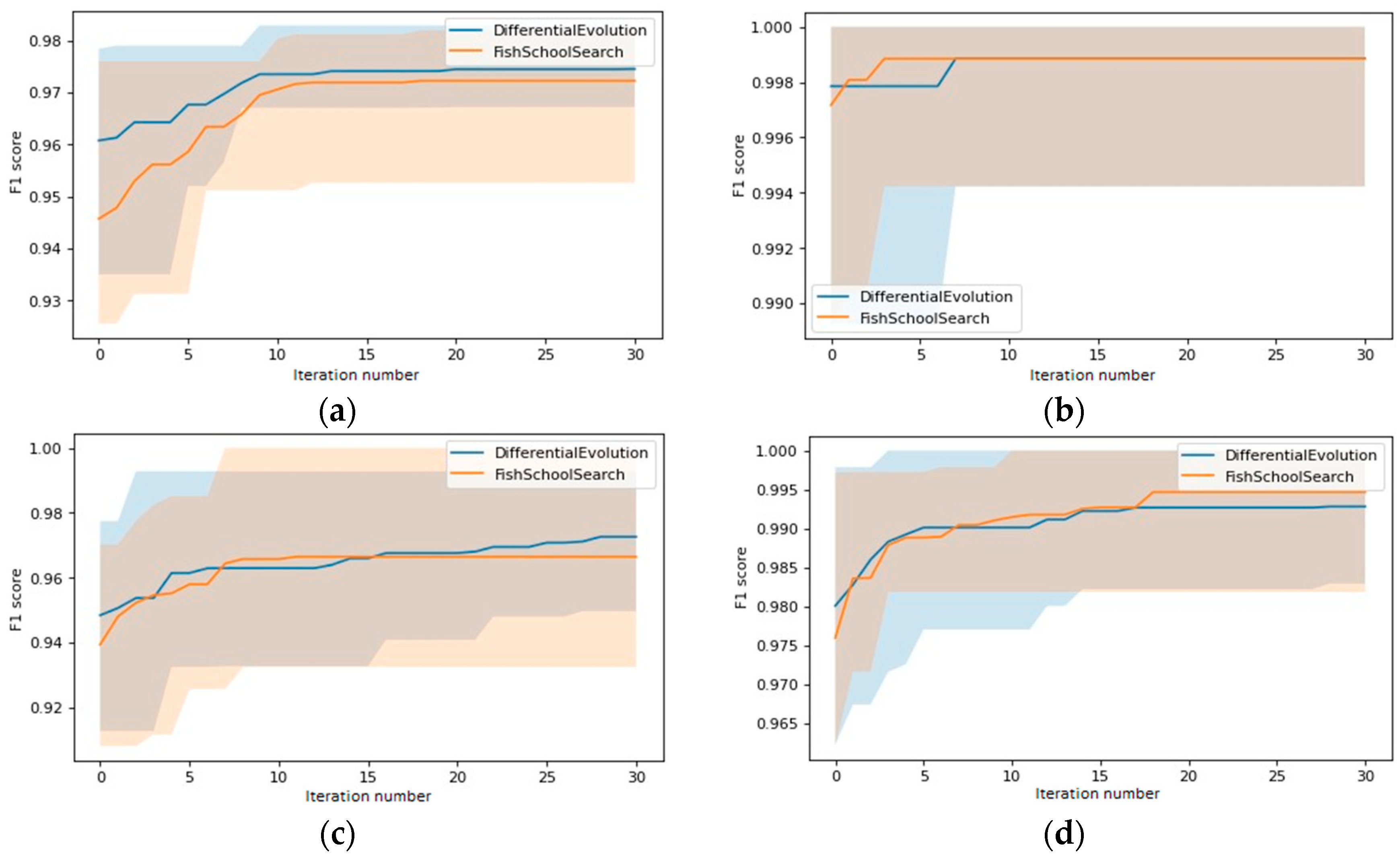
| Differential Evolution (DE) | Fish School Search with Exp. Step Decay (ETFSS) | ||
|---|---|---|---|
| Parameter Title | Value | Parameter Title | Value |
| 0.7 | 0.7 | ||
| 0.3 | 0.7 | ||
| Iteration limit | 30 | Iteration limit | 30 |
| Population size | 20 | Population size | 20 |
| Task Type | Alg. | Accuracy on Testing Data, % | Task | Accuracy on Testing Data, % | ||||||
|---|---|---|---|---|---|---|---|---|---|---|
| Accuracy | Precision | Recall | F1 | Accuracy | Precision | Recall | F1 | |||
| 1 | ELM | 100.00 | 100.00 | 99.99 | 99.99 | 99.89 | 99.54 | 99.25 | 99.34 | |
| DELM | 100.00 | 100.00 | 100.00 | 100.00 | 7 | 100.00 | 100.00 | 100.00 | 100.00 | |
| FELM | 100.00 | 100.00 | 100.00 | 100.00 | 100.00 | 100.00 | 100.00 | 100.00 | ||
| 2 | ELM | 99.82 | 99.72 | 99.82 | 99.77 | 97.05 | 90.08 | 96.18 | 92.14 | |
| DELM | 99.90 | 99.76 | 99.90 | 99.83 | 8 | 97.56 | 97.80 | 97.15 | 97.45 | |
| FELM | 99.90 | 99.76 | 99.90 | 99.83 | 97.89 | 97.05 | 97.52 | 97.23 | ||
| 3 | ELM | 99.93 | 99.95 | 99.96 | 99.95 | 99.35 | 98.26 | 98.37 | 98.24 | |
| DELM | 100.00 | 100.00 | 100.00 | 100.00 | 9 | 99.95 | 99.99 | 99.79 | 99.88 | |
| FELM | 100.00 | 100.00 | 100.00 | 100.00 | 99.95 | 99.99 | 99.79 | 99.88 | ||
| 4 | ELM | 99.95 | 99.30 | 99.98 | 99.59 | 98.23 | 88.95 | 94.62 | 90.75 | |
| DELM | 100.00 | 100.00 | 100.00 | 100.00 | 10 | 99.34 | 95.90 | 98.99 | 97.26 | |
| FELM | 100.00 | 100.00 | 100.00 | 100.00 | 99.07 | 96.27 | 97.16 | 96.65 | ||
| 5 | ELM | 99.98 | 99.76 | 99.99 | 99.83 | 98.24 | 95.66 | 97.74 | 96.30 | |
| DELM | 100.00 | 100.00 | 100.00 | 100.00 | 11 | 99.60 | 99.27 | 99.39 | 99.28 | |
| FELM | 100.00 | 100.00 | 100.00 | 100.00 | 99.60 | 99.27 | 99.75 | 99.47 | ||
| 6 | ELM | 98.67 | 91.40 | 96.07 | 92.84 | |||||
| DELM | 98.76 | 92.22 | 98.01 | 94.54 | ||||||
| FELM | 98.76 | 92.43 | 97.96 | 94.55 | ||||||
Publisher’s Note: MDPI stays neutral with regard to jurisdictional claims in published maps and institutional affiliations. |
© 2022 by the authors. Licensee MDPI, Basel, Switzerland. This article is an open access article distributed under the terms and conditions of the Creative Commons Attribution (CC BY) license (https://creativecommons.org/licenses/by/4.0/).
Share and Cite
Demidova, L.A.; Gorchakov, A.V. Classification of Program Texts Represented as Markov Chains with Biology-Inspired Algorithms-Enhanced Extreme Learning Machines. Algorithms 2022, 15, 329. https://doi.org/10.3390/a15090329
Demidova LA, Gorchakov AV. Classification of Program Texts Represented as Markov Chains with Biology-Inspired Algorithms-Enhanced Extreme Learning Machines. Algorithms. 2022; 15(9):329. https://doi.org/10.3390/a15090329
Chicago/Turabian StyleDemidova, Liliya A., and Artyom V. Gorchakov. 2022. "Classification of Program Texts Represented as Markov Chains with Biology-Inspired Algorithms-Enhanced Extreme Learning Machines" Algorithms 15, no. 9: 329. https://doi.org/10.3390/a15090329
APA StyleDemidova, L. A., & Gorchakov, A. V. (2022). Classification of Program Texts Represented as Markov Chains with Biology-Inspired Algorithms-Enhanced Extreme Learning Machines. Algorithms, 15(9), 329. https://doi.org/10.3390/a15090329