Article

Infrared Image Deblurring Based on Lp-Pseudo-Norm and High-Order Overlapping Group Sparsity Regularization

College of Physics and Information Engineering, Minnan Normal University, Zhangzhou 363000, China
*
Author to whom correspondence should be addressed.
Algorithms 2022, 15(9), 327; https://doi.org/10.3390/a15090327
Submission received: 17 August 2022 / Revised: 6 September 2022 / Accepted: 9 September 2022 / Published: 14 September 2022

Abstract

:
A traditional total variation (TV) model for infrared image deblurring amid salt-and-pepper noise produces a severe staircase effect. A TV model with low-order overlapping group sparsity (LOGS) suppresses this effect; however, it considers only the prior information of the low-order gradient of the image. This study proposes an image-deblurring model (Lp_HOGS) based on the LOGS model to mine the high-order prior information of an infrared (IR) image amid salt-and-pepper noise. An Lp-pseudo-norm was used to model the salt-and-pepper noise and obtain a more accurate noise model. Simultaneously, the second-order total variation regular term with overlapping group sparsity was introduced into the proposed model to further mine the high-order prior information of the image and preserve the additional image details. The proposed model uses the alternating direction method of multipliers to solve the problem and obtains the optimal solution of the overall model by solving the optimal solution of several simple decoupled subproblems. Experimental results show that the model has better subjective and objective performance than Lp_LOGS and other advanced models, especially when eliminating motion blur.

1. Introduction

Images are a primary source of information because they contain large volumes of information and are well-aligned with the cognitive functions of the brain. In the absence of visible light, infrared (IR) radiation generated by an object can be converted into visible IR images using an IR thermal imaging system. The brightness of each pixel in the image corresponds to the change in the intensity of the object’s radiation energy [1]. IR thermal-imaging systems are widely used in biomedicine, military, industrial, and agricultural applications, owing to their strong environmental adaptability, concealment, anti-interference, and identification abilities. However, they have disadvantages such as high noise, low contrast, and blurring. Among the various types of noise, the salt-and-pepper and the Gaussian noises have the greatest impact on IR images [2].
Salt-and-pepper noise is a common random noise exhibiting sparsity in mathematics and statistics. The common methods for removing salt-and-pepper noise include median filter, partial differential equation (PDE) model-based methods, and total variation (TV) model-based methods. Although the median filter method can effectively remove salt-and-pepper noise, it produces deblurred images with incomplete image details [3]. In the last decade, PDE-based models have been developed for various physical applications in image restoration [4]. TV-based models can answer fundamental questions related to image restoration better than other models [5]. The main advantage of this method is that it preserves the image edge. Traditional TV models, including anisotropic TV (ATV) [6] and isotropic TV (ITV) [7], can only approximate the piecewise constant function, causing staircase effects in the restored images [8,9]. Scholars have proposed several variants of the TV model to alleviate the staircase effect. For example, Liu et al. used the L1 norm to describe the statistical characteristics of noise and introduced overlapping group sparsity TV into the salt-and-pepper noise model, achieving good results [10]. However, many non-convex models have achieved better sparse constraints in practical applications than those based on the L1 norm at low sampling rates. Therefore, Yuan and Ghanem proposed a new sparse optimization model (L0TVPADMM) that used an L0 norm as the fidelity term to solve the reconstruction problem based on the TV model [11]. Adam et al. proposed the HNHOTV-OGS method, which combined non-convex high-order total variation and overlapping group sparse regularization [12]. Chartrand proposed a non-convex optimization problem with the minimization of the Lp-pseudo-norm as the objective function [13,14]. Subsequently, Chartrand and Staneva provided a theoretical condition of the Lp-pseudo-norm to recover an arbitrary sparse signal [15]. Wu and Chen [16] and Wen et al. [17] theoretically demonstrated the superiority of methods based on the Lp-pseudo-norm. The Lp-pseudo-norm exhibited a stronger sparse representation ability than the L1 norm. Therefore, it has garnered extensive research interest in recent years [18,19,20,21,22,23]. For example, Lin et al. imposed sparse constraints on the high-order gradients of the image, combined the Lp-pseudo-norm with the total generalized variation model, and proposed an image restoration algorithm that achieved good performance [22]. Based on the mathematical model in [22], Wang et al. replaced the L1 norm with the Lp-pseudo-norm to describe the statistical characteristics of salt-and-pepper noise and proposed an image denoising method based on the Lp-pseudo-norm with low-order overlapping group sparsity (Lp_LOGS) [23].
Among these algorithms, Lp_LOGS performed the best in removing salt-and-pepper noise. However, this method only considers the prior information of the low-order gradient of an image. This study proposes an image-deblurring model based on the Lp_LOGS model to mine the high-order prior information of an IR image containing salt-and-pepper noise, called Lp_HOGS. The second-order TV regularization term was introduced with overlapping group sparsity into the LOGS model, and the Lp-pseudo-norm was retained in the salt-and-pepper noise model. Experimental results show that compared with Lp_LOGS and other advanced models, the proposed Lp_HOGS model demonstrated better peak signal-to-noise ratio (PSNR), structural similarity (SSIM), and gradient magnitude similarity deviation (GMSD). Additionally, the proposed model retained more image details, making the visual effect greater in similarity to the original image. Finally, the proposed model facilitated the subsequent target recognition and tracking processing of the image.

2. Materials and Methods

2.1. The Background to Deblurring Algorithms

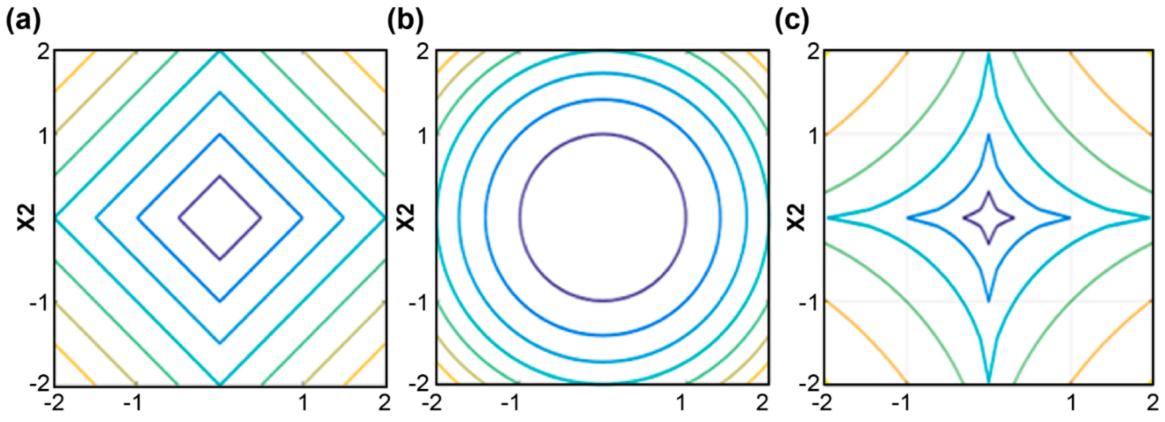
2.1.1. The Lp-Pseudo-Norm

The Lp-pseudo-norm represents the distance in the vector space and is a generalized concept of “distance.” The Lp norm of the matrix X is defined as X p = ( i = 1 M j = 1 N | X i j | p ) 1 p , when p is 1 and 2, and corresponds to the L1 and L2 norms, respectively. The Lp-pseudo-norm is defined as X p p = i = 1 M j = 1 N | X i j | p . This study focused on the case where 0 < p < 1 . The contour maps of different norms are presented in Figure 1. The Lp-pseudo-norm has one more degree of freedom than the L1 and L2 norms, and the contour of the Lp-pseudo-norm was closest to the coordinate axis. Hence, the solution has a higher probability of being a point that is on or close to the axis. The Lp-pseudo-norm has a stronger sparse representation ability based on these reasons. Therefore, the Lp-pseudo-norm was introduced into the model for salt-and-pepper denoising in this study.

2.1.2. The Overlapping Group Sparse TV Regularization Term

The overlapping group sparse TV regularization term is expressed as:
R OGSTV ( F ) = φ ( K h F ) + φ ( K v F )
where represents the convolution operator, K h = [ 1 , 1 ] is the first-order horizontal difference convolution kernel, F is the original image, and K v = [ 1 , 1 ] T is the first-order vertical difference convolution kernel. φ ( V ) is the function for calculating the combined gradient and is expressed as:
φ ( V ) = i = 1 N j = 1 N V ˜ i , j , K , K 2 ( V N × N )
where V ˜ i , j , K , K represents the overlapping group sparsity matrix, which is defined as:
V ˜ i , j , K , K = ( V i K l , j K l V i K l , j K l + 1 V i K l , j + K r V i K l + 1 , j K l V i K l + 1 , j K l + 1 V i K l + 1 , j + K r V i + K r , j K l V i + K r , j K l + 1 V i + K r , j + K r ) K × K
where K represents the length or width of the matrix of the combined gradient, K l = K 1 2 ,   K r = K 2 , and . means round down to the nearest integer.
As indicated in Equation (3), the overlapping group sparse TV regularization term uses the gradient of the pixel point ( i , j ) as the center, constructs a K × K matrix, combines it using the L2 norm, and replaces the independent gradient of the pixel point. Compared with the traditional anisotropic TV regularization term, the overlapping group sparse TV regularization term fully mines the gradient information of each pixel and considers the structural information of the image, thereby increasing the difference between the smooth and the edge areas of the image.

2.1.3. The Lp_LOGS Model

Blurred images are generally considered images corrupted by blur kernels and additive noise. They can be represented by the following linear mathematical model:
G = H F + η
where G represents the degraded image to be deblurred, H is the blur kernel, and η is the additive noise, specifically the salt-and-pepper noise in this study.
The application of the Lp_LOGS model to solve F is an ill-posed inverse problem, which is expressed as:
F = arg min F H F G p p + μ [ R OGSTV ( F ) ] ,
where H F G p p is the fidelity term, R OGSTV ( F ) is the prior term, and μ is the balance coefficient used to balance the prior and the fidelity terms.
The Lp_LOGS model leverages the Lp-pseudo-norm and overlapping group sparse TV regularization term, vastly outperforming the traditional ATV model in terms of deblurring. However, the Lp_LOGS model only considers the overlapping group sparse constraints of the low-order gradient information of the image.
To mine the prior information of the high-order gradient of an image, the second-order overlapping group sparse TV regularization term was introduced into the Lp_LOGS model. The proposed novel deblurring model is expressed as:
F = arg min F H F G p p + μ 1 [ φ ( K h F ) ] + μ 2 [ φ ( K v F ) ] + μ 3 [ φ ( K h K h F ) ] + μ 4 [ φ ( K v K v F ) ] + μ 5 [ φ ( K v K h F ) ] ,
where μ i ( i = 1 , 2 , 3 , 4 , 5 ) represents the balance coefficient, K h K h is the second-order horizontal difference convolution kernel, K v K v is the second-order vertical difference convolution kernel, and K v K h is the second-order mixed difference convolution kernel.
This model was named Lp_HOGS to represent a deblurring model based on the Lp-pseudo-norm with high-order overlapping group sparsity regularization.

2.2. The Solution of the Lp_HOGS Model

The alternating direction method of multipliers (ADMM) was used to solve the Lp_HOGS model. When solving this model, ADMM transformed the original complex problem into several relatively simple subproblems by introducing decoupling variables.
According to the ADMM solution framework, the intermediate variables Z 0 = H F G , Z 1 = K h F , Z 2 = K v F , Z 3 = K h K h F , Z 4 = K v K v F , Z 5 = K v K h F , were included and the original problem was transformed into an optimization problem with constraints, which is expressed as:
J = m i n Z 0 Z 5 { Z 0 p p + μ 1 [ φ ( Z 1 ) ] + μ 2 [ φ ( Z 2 ) ] + μ 3 [ φ ( Z 3 ) ] + μ 4 [ φ ( Z 4 ) ] + μ 5 [ φ ( Z 5 ) ] } .
The corresponding Lagrange multiplier Λ i ( i = 0 , 1 , 2 , 3 , 4 , 5 ) and quadratic penalty coefficient β i ( i = 0 , 1 , 2 , 3 , 4 , 5 ) were used to transform Equation (7) into an unconstrained optimization problem, i.e., the augmented Lagrange objective function of the original problem, which is expressed as:
J = m a x Λ 0 Λ 5 { m i n F , Z 0 Z 5 { Z 0 p p β 0 Λ 0 , Z 0 ( H F G ) + β 0 2 Z 0 ( H F G ) 2 2 + μ 1 [ φ ( Z 1 ) ] β 1 Λ 1 , Z 1 K h F + β 1 2 Z 1 K h F 2 2 + μ 2 [ φ ( Z 2 ) ] β 2 Λ 2 , Z 2 K v F + β 2 2 Z 2 K v F 2 2 + μ 3 [ φ ( Z 3 ) ] β 3 Λ 3 , Z 3 K h K h F + β 3 2 Z 3 K h K h F 2 2 + μ 4 [ φ ( Z 4 ) ] β 4 Λ 4 , Z 4 K v K v F + β 4 2 Z 4 K v K v F 2 2 + μ 5 [ φ ( Z 5 ) ] β 5 Λ 5 , Z 5 K v K h F + β 5 2 Z 5 K v K h F 2 2 } } ,
where X , Y represents the inner product of the X , Y matrices.
0 = β i 2 Λ i 2 2 β i 2 Λ i 2 2 ( i = 0 , 1 , 2 , 3 , 4 , 5 )
Subsequently, adding Equation (9) to the right side of Equation (8) obtains:
J = m a x Λ 0 Λ 5 { m i n F , Z 0 Z 5 { Z 0 p p + β 0 2 Z 0 ( H F G ) Λ 0 2 2 β 0 2 Λ 0 2 2 + μ 1 [ φ ( Z 1 ) ] + β 1 2 Z 1 K h F Λ 1 2 2 β 1 2 Λ 1 2 2 + μ 2 [ φ ( Z 2 ) ] + β 2 2 Z 2 K v F Λ 2 2 2 β 2 2 Λ 2 2 2 + μ 3 [ φ ( Z 3 ) ] + β 3 2 Z 3 K h K h F Λ 3 2 2 β 3 2 Λ 3 2 2 + μ 4 [ φ ( Z 4 ) ] + β 4 2 Z 4 K v K v F Λ 4 2 2 β 4 2 Λ 4 2 2 + μ 5 [ φ ( Z 5 ) ] + β 5 2 Z 5 K v K h F Λ 5 2 2 β 5 2 Λ 5 2 2 } } .
Each subproblem must first be solved to solve the objective function. As the introduced variables Z i ( i = 0 , 1 , 2 , 3 , 4 , 5 ) , Λ i ( i = 0 , 1 , 2 , 3 , 4 , 5 ) , and F were decoupled, the objective function corresponding to the subproblems of F became:
J F = m i n F { β 0 2 Z 0 ( H F G ) Λ 0 2 2 + β 1 2 Z 1 K h F Λ 1 2 2 + β 2 2 Z 2 K v F Λ 2 2 2 + β 3 2 Z 3 K h K h F Λ 3 2 2 + β 4 2 Z 4 K v K v F Λ 4 2 2 + β 5 2 Z 5 K v K h F Λ 5 2 2 } .
The convolution theorem was used to apply the Fourier transform to both sides of Equation (11), which is expressed as:
J F ¯ = m i n F ¯ { β 0 2 ( H ¯ F ¯ G ¯ ) + Λ ¯ 0 Z ¯ 0 2 2 + β 1 2 K ¯ h F ¯ + Λ ¯ 1 Z ¯ 1 2 2 + β 2 2 K ¯ v F ¯ + Λ ¯ 2 Z ¯ 2 2 2 + β 3 2 K ¯ h K ¯ h F ¯ + Λ ¯ 3 Z ¯ 3 2 2 + β 4 2 K ¯ v K ¯ v F ¯ + Λ ¯ 4 Z ¯ 4 2 2 + β 5 2 K ¯ v K ¯ h F ¯ + Λ ¯ 5 Z ¯ 5 2 2 } ,
where denotes the dot product operator and X ¯ is the Fourier transform of the X matrix.
The partial derivative of F ¯ can be calculated using:
J F ¯ F ¯ = β 0 H ¯ * ( ( H ¯ F ¯ G ¯ ) + Λ ¯ 0 Z ¯ 0 ) + β 1 K ¯ h * ( K ¯ h F ¯ + Λ ¯ 1 Z ¯ 1 ) + β 2 K ¯ v * ( K ¯ v F ¯ + Λ ¯ 2 Z ¯ 2 ) + β 3 ( K ¯ h K ¯ h ) * ( K ¯ h K ¯ h F ¯ + Λ ¯ 3 Z ¯ 3 ) + β 4 ( K ¯ v K ¯ v ) * ( K ¯ v K ¯ v F ¯ + Λ ¯ 4 Z ¯ 4 ) + β 5 ( K ¯ v K ¯ h ) * ( K ¯ v K ¯ h F ¯ + Λ ¯ 5 Z ¯ 5 ) ,
where X * represents the conjugate matrix of the X matrix.
Here, Equation (13) is assumed to be equal to a zero matrix and can be rearranged as:
L H S F ¯ = R H S
where
L H S = β 0 H ¯ * H ¯ + β 1 K ¯ h * K ¯ h + β 2 K ¯ v * K ¯ v + β 3 ( K ¯ h K ¯ h ) * ( K ¯ h K ¯ h ) + β 4 ( K ¯ v K ¯ v ) * ( K ¯ v K ¯ v ) + β 5 ( K ¯ v K ¯ h ) * ( K ¯ v K ¯ h )
and
R H S = β 0 H ¯ * ( Z ¯ 0 + G ¯ Λ ¯ 0 ) + β 1 K ¯ h * ( Z ¯ 1 Λ ¯ 1 ) + β 2 K ¯ v * ( Z ¯ 2 Λ ¯ 2 ) + β 3 ( K ¯ h K ¯ h ) * ( Z ¯ 3 Λ ¯ 3 ) + β 4 ( K ¯ v K ¯ v ) * ( Z ¯ 4 Λ ¯ 4 ) + β 5 ( K ¯ v K ¯ h ) * ( Z ¯ 5 Λ ¯ 5 ) .
The updated formula of F is expressed as:
F = 1 ( R H S . / L H S )
where . / represents the dot division operator and 1 ( X ) is the inverse Fourier transform of X .
The objective function to solve the subproblem Z 0 is expressed as:
J Z 0 = m i n Z 0 {   Z 0 p p + β 0 2 Z 0 ( H F G ) Λ 0 2 2   }
According to the Lp shrinkage operator:
s h r i n k p ( ξ , τ ) = m a x { | ξ | τ 2 p | ξ | p 1 , 0 } ξ | ξ |
The updated formula of Z 0 is expressed as:
Z 0 = s h r i n k p ( ( H F G ) + Λ 0 , 1 β 0 ) = m a x { | ( H F G ) + Λ 0 | β 0 p 2 | ( H F G ) + Λ 0 | p 1 , 0 } ( H F G ) + Λ 0 | ( H F G ) + Λ 0 | .
Additionally, the objective function of the subproblem Z 1 is expressed as:
J Z 1 = m i n Z 1 {   μ 1 [ φ ( Z 1 ) ] + β 1 2 Z 1 K h F Λ 1 2 2 }
According to the ADMM algorithm, the updated formula of Z 1 is expressed as:
Z 1 ( n + 1 ) ( k + 1 ) = m a t { [ I + μ 1 β 1 D 2 ( Z 1 ( n ) ( k + 1 ) ) ] 1 v e c ( Z 1 ( 0 ) ( k + 1 ) ) } ( Z 1 ( 0 ) ( k + 1 ) = K h F + Λ 1 ( k ) )
where m a t is the vector matricization operator, v e c is the matrix vectorization operator, I N 2 × N 2 is the identity matrix, and D N 2 × N 2 is the diagonal matrix with diagonal elements.
[ D ( U ) ] m , m = i = K l K r j = K l K r { k 1 = K l K r k 2 = K l K r | U m i + k 1 , m J + k 2 | 2 } 1 2
where U represents an arbitrary matrix.
Similarly, the updated formulas of Z 2 Z 5 can be obtained, which are expressed as:
{ Z 2 ( n + 1 ) ( k + 1 ) = m a t { [ I + μ 2 β 2 D 2 ( Z 2 ( n ) ( k + 1 ) ) ] 1 v e c ( Z 2 ( 0 ) ( k + 1 ) ) } ( Z 2 ( 0 ) ( k + 1 ) = K v F + Λ 2 ( k ) ) Z 3 ( n + 1 ) ( k + 1 ) = m a t { [ I + μ 3 β 3 D 2 ( Z 3 ( n ) ( k + 1 ) ) ] 1 v e c ( Z 3 ( 0 ) ( k + 1 ) ) } ( Z 3 ( 0 ) ( k + 1 ) = K h K h F + Λ 3 ( k ) ) Z 4 ( n + 1 ) ( k + 1 ) = m a t { [ I + μ 4 β 4 D 2 ( Z 4 ( n ) ( k + 1 ) ) ] 1 v e c ( Z 4 ( 0 ) ( k + 1 ) ) } ( Z 4 ( 0 ) ( k + 1 ) = K v K v F + Λ 4 ( k ) ) Z 5 ( n + 1 ) ( k + 1 ) = m a t { [ I + μ 5 β 5 D 2 ( Z 5 ( n ) ( k + 1 ) ) ] 1 v e c ( Z 5 ( 0 ) ( k + 1 ) ) } ( Z 5 ( 0 ) ( k + 1 ) = K v K h F + Λ 5 ( k ) ) .
The objective function to solve subproblem Λ 0 is expressed as:
J Λ 0 = m a x Λ 0 {   β 0 Λ 0 , Z 0 ( H F G )   }
According to the gradient ascent method, the updated formula of Λ 0 is expressed as:
J Λ 0 = m a x Λ 0 {   β 0 Λ 0 , Z 0 ( H F G )   }
where γ is the learning rate.
The objective function to solve subproblem Λ 1 is expressed as:
J Λ 1 = m a x Λ 1 {   β 1 Λ 1 , Z 1 K h F   }
According to the gradient ascent method, the updated formula of Λ 1 is expressed as:
Λ 1 ( k + 1 ) = Λ 1 ( k ) + γ β 1 ( K h F Z 1 ( k + 1 ) )
Similarly, the updated formulas of Λ 2 Λ 5 can be obtained, which are expressed as:
{ Λ 2 ( k + 1 ) = Λ 2 ( k ) + γ β 2 ( K v F Z 2 ( k + 1 ) ) Λ 3 ( k + 1 ) = Λ 3 ( k ) + γ β 3 ( K h K h F Z 3 ( k + 1 ) ) Λ 4 ( k + 1 ) = Λ 4 ( k ) + γ β 4 ( K v K v F Z 4 ( k + 1 ) ) Λ 5 ( k + 1 ) = Λ 5 ( k ) + γ β 5 ( K v K h F Z 5 ( k + 1 ) ) .
Hence, the subproblems are solved.
Given the above descriptions, the specific description of the Lp_HOGS algorithm is shown in Algorithm 1.
Algorithm 1. Lp_ HOGS
Input Observed image G .
Output Deblurred image F .
Initialize:
k = 0 , t o l = 1 0 4 , e r r = 1 , p , γ , F = 0 , Z i = 0 , Λ i = 0 , μ j , β i ( i = 0 , 1 , , 5 ; j = 1 , 2 , , 5 ) .
1: If  e r r > t o l do
2:  Use Equations (15)–(17) to update F ;
3:  Use Equation (20) to update Z 0 ;
4:  Use Equations (22) and (24) to update Z i ( i = 1 , 2 , , 5 ) ;
5:  Use Equation (26) to update Λ 0 ;
6:  Use Equations (28) and (29) to update Λ i ( i = 1 , 2 , , 5 ) ;
7:   k = k + 1 ;
8:   e r r = F ( k + 1 ) F ( k ) 2 / F ( k ) 2 ;
9: End if
10: Return  F ( k ) as F .
where tol represents the threshold.

3. Results and Discussion

The IR test images used in the experiment were downloaded from the publicly available datasets found at http://adas.cvc.uab.es/elektra/datasets/far-infra-red/ (accessed on 5 January 2022) and http://www.dgp.toronto.edu/~{}nmorris/data/IRData/ (accessed on 5 January 2022). This study evaluated the quality of the denoised images from subjective and objective aspects. The objective evaluation metrics used in this study are PSNR, SSIM, and GMSD, which are defined using Equations (30)–(32), respectively:
PSNR = 10 log 10 ( 255 2 1 M N i = 1 M j = 1 N x i j y i j 1 2 ) ( dB ) ,
SSIM = ( 2 u X u Y + ( 255 k 1 ) 2 ) ( 2 σ X Y + ( 255 k 2 ) 2 ) ( u X 2 + u Y 2 + ( 255 k 1 ) 2 ) ( σ X 2 + σ Y 2 + ( 255 k 2 ) 2 ) ,
where X and Y are the original and the restored image, respectively. u X and u Y represent the mean values of X and Y , respectively. σ X 2 and σ Y 2 represent the variances of X and Y , respectively. σ X Y represents the covariance of X and Y . k 1 and k 2 are constants to ensure that SSIM is not zero.
GMSD = 1 M N i = 1 M j = 1 N { [ GMS ] i , j 1 M N i = 1 M j = 1 N [ GMS ] i , j } 2 ,
where
[ GMS ] i , j = 2 [ m X ] i , j [ m Y ] i , j + c [ m X ] i , j 2 + [ m Y ] i , j 2 + c .
where c is a constant to ensure that the denominator is a non-zero number. [ m X ] i , j and [ m Y ] i , j refer to the gradient amplitude of the image in the horizontal and vertical directions, respectively.
Larger PSNR, closer-to-1 SSIM, and smaller GMSD values indicate better deblurring performance.
The variable parameters were preset before the experiment to focus on PSNR optimization before optimizing SSIM and GMSD. The variable parameters of the Lp_HOGS model were set as follows:
The maximum number of iterations and the learning rate γ were set to 500 and 0.618, respectively.
For each model, the balance coefficient μ j ( j = 1 , 2 , , 5 ) , the quadratic penalty coefficient β i ( i = 0 , 1 , , 5 ) , and the Lp-pseudo-norm p were manually optimized to achieve the best deblurring effect on the IR image and ensure a fair experiment.
A sensitivity experiment analysis revealed that K was essential and the image quality indicators were optimal when K = 3 was the size of the matrix. The structured information of the image could not be fully mined if the value of K was insignificant. Conversely, unstructured information could be introduced if the value was excessively large.

3.1. The Comparison of Lp_HOGS with Lp_LOGS

Lp_HOGS and Lp_LOGS were compared to verify the effect of adding the second-order overlapping group sparse TV regularization term. We added 30%, 40%, and 50% salt-and-pepper noise to the Gaussian, box, and motion blurs to obtain nine degradation combinations and compared the quality of the deblurred images. Nine distinct IR images were selected as the test images. Images of a passerby, a station, a truck, a car, and some buildings were 384 × 288 pixels each, and images of a garden, some stairs, a corridor, and a zebra crossing were 506 × 408 pixels each.

3.1.1. The Gaussian Blur

The noise was generated by the MATLAB built-in function “noise (I, type, parameters)”. For example, 30% of the salt-and-pepper noise was set to noise (I, ‘salt & Pepper’, 0.3). We included 30%, 40%, and 50% of the salt-and-pepper noise in the test images with a 7 × 7 Gaussian blur. The experimental results are summarized in Table 1.
The three performance indicators obtained by the Lp_HOGS model were higher than those of the Lp_LOGS model; thereby demonstrating that the proposed method achieved better deblurring and denoising effects. The Lp_HOGS model achieved average PSNR values that were 0.304, 0.784, and 1.287 dB higher than those of the Lp_LOGS model when the salt-and-pepper noise was 30%, 40%, and 50%, respectively. Therefore, the Lp_HOGS model had a greater advantage when the noise levels increased.
The passerby images with different degrees of degradation are shown in Figure 2. The deblurring effects using Lp_LOGS and Lp_HOGS are compared in Figure 3.
A comparison of Figure 2a,c with Figure 3b,c revealed that the image deblurred by Lp_LOGS had more speckle noise than the one deblurred by Lp_HOGS. The images in the red boxes in Figure 3b,c were enlarged to further visualize the difference between the two and the results are displayed in Figure 3e,f, respectively.
The right half was a largely smooth area in Figure 3e,f. Figure 3f had less salt-and-pepper noise compared with Figure 3e and its visual effect was closer to that of the original image. The left half was mostly the edge area, therefore it was difficult to see the denoising effect. However, Figure 3f retained more details. For example, the lines of the iron fence are clearer and more continuous. Overall, the visual effect of Figure 3f was closer to that of the original image, indicating that the deblurring performance of Lp_HOGS under the Gaussian blur was better than that of Lp_LOGS. Lp_HOGS also preserved more details while suppressing the staircase effect of deblurred images.

3.1.2. The Box Blur

We added 30%, 40%, and 50% salt-and-pepper noise to the test images with a 7 × 7 box blur. The experimental results are listed in Table 2.
The three performance indicators obtained by the Lp_HOGS model were higher than those obtained by the Lp_LOGS model. The Lp_HOGS model achieved average PSNR values that were 0.362, 0.805, and 1.356 dB higher than those of the Lp_LOGS model when the salt-and-pepper noise was 30%, 40%, and 50%, respectively. In terms of the difference in the PSNR value, Lp_HOGS had a marginally greater advantage over Lp_LOGS in the 7 × 7 box blur than in the 7 × 7 Gaussian blur.
A station image with different degrees of degradation is shown in Figure 4. The images that were deblurred by Lp_LOGS and Lp_HOGS are compared in Figure 5.
A comparison of Figure 4a,c with Figure 5b,c revealed satisfactory overall deblurring effects of Lp_LOGS and Lp_HOGS on images with the box blur. However, the image deblurred by Lp_LOGS contained more speckle noise than the image deblurred by Lp_HOGS. The images in the red boxes in Figure 5b,c are enlarged in Figure 5e,f, respectively.
The upper halves of Figure 5e,f were mostly smooth areas. The model used to create Figure 5f removed salt-and-pepper noise more thoroughly than that used on Figure 5e and its visual effect was closer to the original image. The lower half mostly contained the edge area. Thus, the denoising effect was not evident. However, Figure 5f retained more detail from the original image. For example, the car logo is clearer. Overall, the visual effect of Figure 5f was closer to that of the original image, indicating that Lp_HOGS exhibited better deblurring performance than Lp_LOGS under the box blur. It was also reconfirmed that Lp_HOGS preserved more detail while suppressing the staircase effect of the deblurred images.

3.1.3. The Motion Blur

Finally, 30%, 40%, and 50% salt-and-pepper noise were added to the test images with a 7 × 7 motion blur. The experimental results are listed in Table 3.
The three performance indicators obtained by the Lp_HOGS model were higher than those obtained by the Lp_LOGS model. The Lp_HOGS model achieved average PSNR values that were 1.387, 1.774, and 2.372 dB higher than those of the Lp_LOGS model when the salt-and-pepper noise was 30%, 40%, and 50%, respectively. The difference in the PSNR values showed that Lp_HOGS had more obvious advantages over Lp_LOGS in the motion blur than in the Gaussian and box blurs.
The images of a truck with different degrees of degradation are shown in Figure 6. The deblurring effects of Lp_LOGS and Lp_HOGS are compared in Figure 7.
A comparison of Figure 6a,c with Figure 7b,c revealed that Lp_LOGS and Lp_HOGS achieved satisfactory deblurring effects in terms of motion blur. Furthermore, the performance edge of the proposed model was similar to that under the Gaussian and the box blurs. The deblurring effects are depicted in Figure 7b,c,e,f.

3.2. The Comparison with Other Methods

This section compares the proposed model with existing models, including ATV [4], ITV [5], L0TVPADMM [9], and HNHOTV-OGS [10]. Nine distinct IR images were selected as test images. The truck, the buildings, the car, and the figure images were 384 × 288 pixels, and the garden, the stairs, the corridor, the road, and the zebra crossing images were 506 × 408 pixels. The experimental results are listed in Table 4 and the unit of PSNR as dB.
ITV performed the worst, whereas Lp_HOGS outperformed the other four methods in terms of PSNR, SSIM, and GMSD. The PSNR of Lp_HOGS under 30%, 40%, and 50% salt-and-pepper noise was at least 1.2 dB higher than that of L0TVPADMM, which had the second-best PSNR. Therefore, the proposed Lp_HOGS model achieved better performance for removing salt-and-pepper noise than the other state-of-the-art methods. In addition, the IR image after deblurring obtained a better visual effect, which is conducive to subsequent image analysis and processing.

4. Conclusions

This study proposed an image-deblurring model based on the LOGS model to mine the high-order prior information of an IR image containing salt-and-pepper noise. The LOGS regularization term was investigated, combining the advantage of the Lp-pseudo-norm in describing salt-and-pepper noise with replacing the low-order term with a high-order term. The proposed IR image-deblurring model (Lp_HOGS) successfully deblurred an IR image under salt-and-pepper noise. Lp_HOGS achieved average PSNR values that were 0.304, 0.784, and 1.287 dB higher for salt-and-pepper noise at 30%, 40% and 50%, respectively, than those of the Lp_LOGS model for a Gaussian blur. Similarly, Lp_HOGS was 0.362, 0.805, and 1.356 dB higher for the box blur and 1.387, 1.774, and 2.372 dB higher for the motion blur. The findings of this study resulted in the following conclusions:
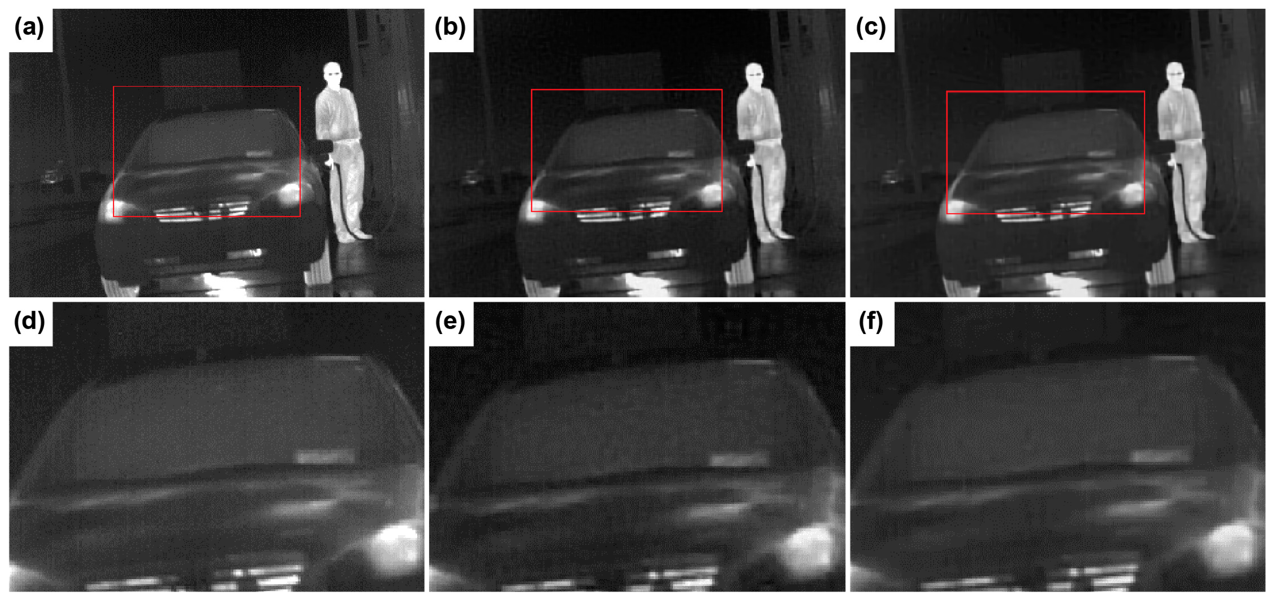
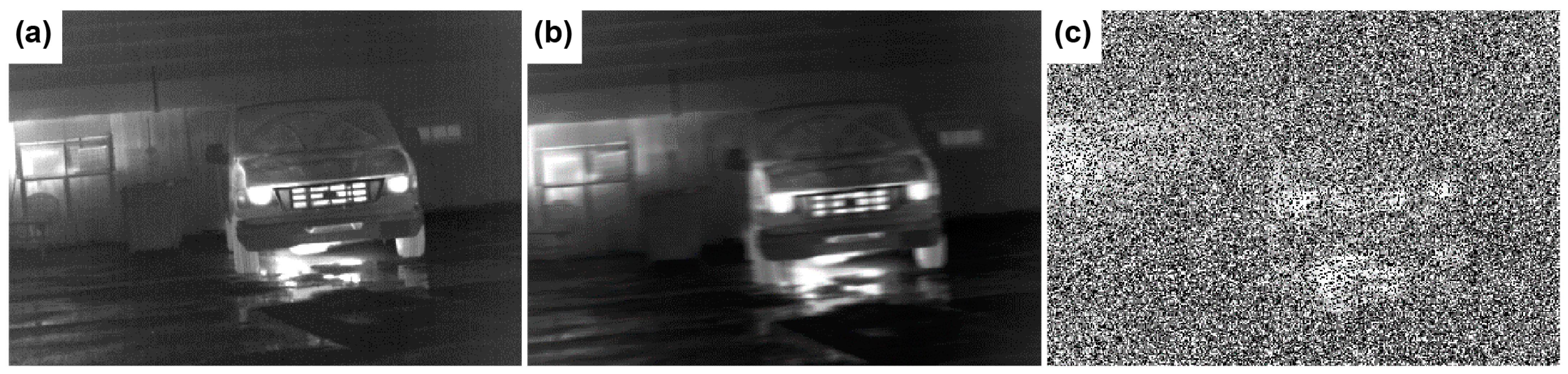
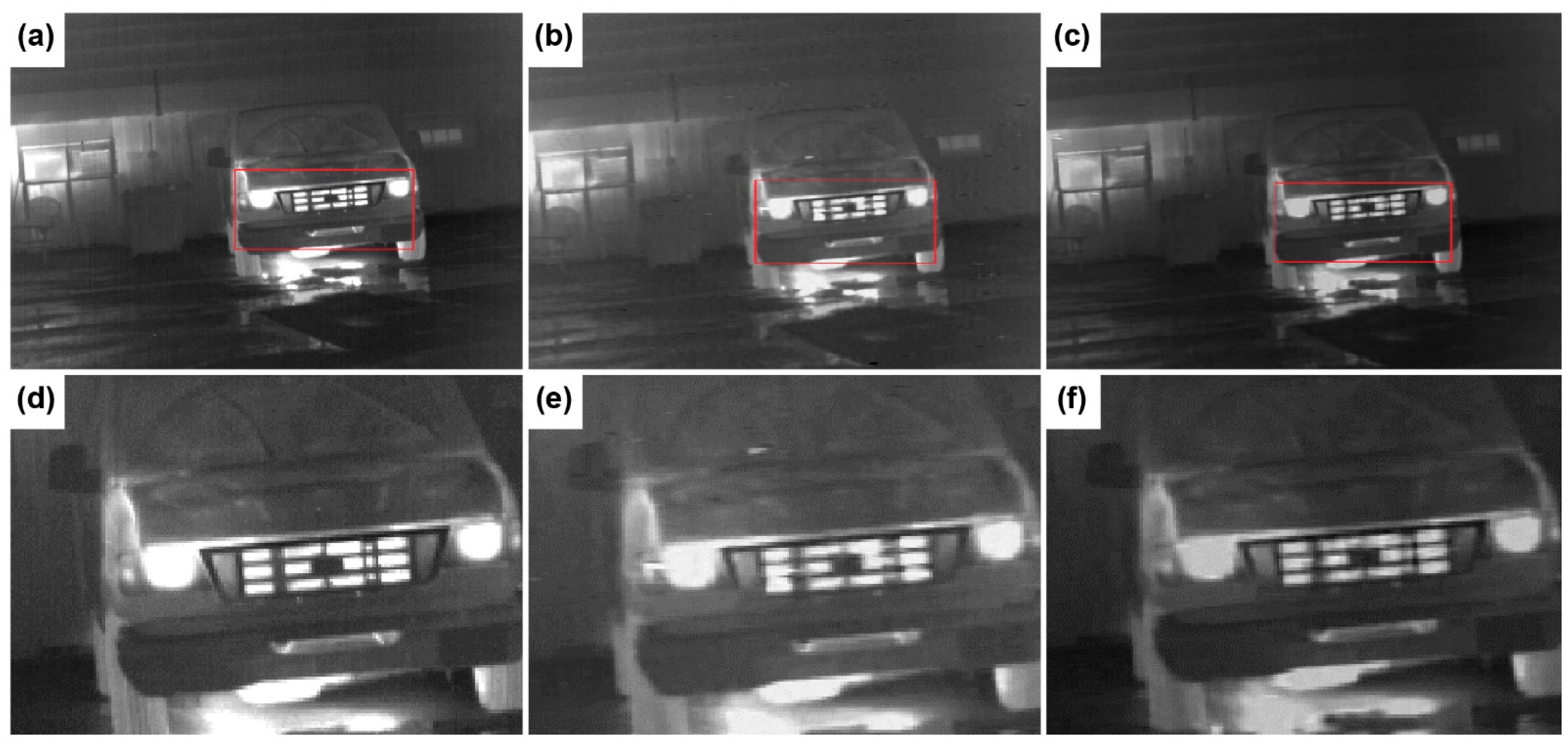
  • Upon adding the Gaussian blur and different levels of salt-and-pepper noise to a given test image, the Lp_HOGS model exhibited a better deblurring effect than the existing models. This result implies that the Lp-pseudo-norm had a stronger sparse representation ability and the overlapping group sparsity regularization term increased the difference between the smooth and the edge areas of an image.
  • Upon adding the different types of blur and levels of salt-and-pepper noise to a given test image, Lp_HOGS yielded stronger indicators than Lp_LOGS. This advantage became greater as the noise level increased. Therefore, the high-order prior information of the image improved the quality of the deblurred IR images and the stability of salt-and-pepper noise removal.
  • The advantage of Lp_HOGS over Lp_LOGS was most obvious in terms of the motion blur, indicating that adding the prior constraints of the high-order gradient to the model could significantly improve the IR image deblurring effect amid the motion blur.
A limitation of this approach is that the application of the Lp_HOGS model is time-consuming. In our future work, we will accelerate the process by introducing accelerated ADMM to improve the performance and efficiency of the proposed method. Nevertheless, the proposed Lp_HOGS model provides a new approach to reduce the salt-and-pepper noise impact on IR images.

Author Contributions

Conceptualization, Z.Y. and Y.C.; Methodology, Z.Y.; Software, Z.Y. and J.H.; Validation, Z.Y. and X.O.; Formal analysis, Z.Y.; Investigation, Z.Y. and J.H.; Resources, Y.C.; Data curation, Z.Y. and X.O.; Writing—original draft preparation, Z.Y. and X.O.; Writing—review and editing, Z.Y. and Y.C.; Visualization, Z.Y.; Supervision, Y.C.; Project administration, Y.C.; Funding acquisition, Y.C. All authors have read and agreed to the published version of the manuscript.

Funding

This research was funded by the Natural Science Foundation Project of Fujian Province, grant numbers 2020J05169 and 2020J01816; Principal Foundation of Minnan Normal University, grant number KJ19019; and High-Level Science Research Project of Minnan Normal University, grant number GJ19019.

Data Availability Statement

The data presented in this study are openly available at http://adas.cvc.uab.es/elektra/datasets/far-infra-red/ (accessed on 5 January 2022), http://www.dgp.toronto.edu/~{}nmorris/data/IRData/ (accessed on 5 January 2022), and http://adas.cvc.uab.es/elektra/datasets/far-infra-red/ (accessed on 5 January 2022). Additionally, the perfect code data for the proposed method in this paper are available upon request from the corresponding author.

Acknowledgments

Thank you to X.L. of the University of Electronic Science and Technology of China for sharing the FTV4Lp code.

Conflicts of Interest

The authors declare no conflict of interest. The funders had no role in the design of the study; in the collection, analyses, or interpretation of data; in the writing of the manuscript; or in the decision to publish the results.

References

  1. Li, J.; Yang, W.; Zhang, X. Infrared Image Processing, Analysis, and Fusion; Science Press: Beijing, China, 2009; pp. 7–12. Available online: https://max.book118.com/html/2019/0105/5210100330001344.shtm (accessed on 15 January 2022).
  2. Fan, Z.; Bi, D.; He, L.; Ma, S. Noise suppression and details enhancement for infrared image via novel prior. Infrared Phys. Technol. 2016, 74, 44–52. [Google Scholar] [CrossRef]
  3. Faragallah, O.S.; Ibrahem, H.M. Adaptive switching weighted median filter framework for suppressing salt-and-pepper noise. Int. J. Electron. Commun. 2016, 70, 1034–1040. [Google Scholar] [CrossRef]
  4. Afraites, L.; Hadri, A.; Laghrib, A. A denoising model adapted for impulse and Gaussian noises using a constrained-PDE. Inverse Probl. 2020, 36, 025006. [Google Scholar] [CrossRef]
  5. Lim, H.; Williams, T.N. A Non-standard Anisotropic Diffusion for Speckle Noise Removal. Syst. Cybern. Inform. 2007, 5, 12–17. Available online: http://www.iiisci.org/Journal/pdv/sci/pdfs/P610066.pdf (accessed on 16 August 2022).
  6. Osher, S.; Burger, M.; Goldfarb, D.; Jinjun, X.; Wotao, Y. An iterative regularization method for total variation-based image restoration. Multiscale Model. Simul. 2005, 4, 460–489. [Google Scholar] [CrossRef]
  7. Peng, Z.; Chen, Y.; Pu, T.; Wang, Y.; He, Y. Image denoising based on sparse representation and regularization constraint: A Review. J. Data Acquis. Process. 2018, 33, 1–11. Available online: http://www.cnki.com.cn/Article/CJFDTotal-SJCJ201801001.htm (accessed on 16 December 2021).
  8. Li, S.; He, Y.; Chen, Y.; Liu, W.; Yang, X.; Peng, Z. Fast multi-trace impedance inversion using anisotropic total p-variation regularization in the frequency domain. J. Geophys. Eng. 2018, 15, 2171–2182. [Google Scholar] [CrossRef]
  9. Wu, H.; He, Y.; Chen, Y.; Shu, L.; Peng, Z. Seismic acoustic impedance inversion using mixed second-order fractional ATpV regularization. IEEE Access 2020, 8, 3442–3452. [Google Scholar] [CrossRef]
  10. Liu, G.; Huang, T.Z.; Liu, J.; Lv, X.G. Total variation with overlapping group sparsity for image deblurring under impulse noise. PLoS ONE 2015, 10, e0122562. [Google Scholar] [CrossRef]
  11. Yuan, G.; Ghanem, B. l0tv: A new method for image restoration in the presence of impulse noise. In Proceedings of the IEEE Conference on Computer Vision and Pattern Recognition, Boston, MA, USA, 7–12 June 2015; pp. 5369–5377. [Google Scholar]
  12. Adam, T.; Paramesran, R. Image denoising using combined higher order non-convex total variation with overlapping group sparsity. J. Multidimens. Syst. Signal Process. 2019, 30, 503–527. [Google Scholar] [CrossRef]
  13. Chartrand, R. Exact reconstruction of sparse signals via nonconvex minimization. IEEE Signal Process. Lett. 2007, 14, 707–710. [Google Scholar] [CrossRef]
  14. Chartrand, R. Shrinkage mappings and their induced penalty functions. In Proceedings of the 2014 IEEE International Conference on Acoustics, Speech and Signal Processing (ICASSP), Florence, Italy, 4–9 May 2014; pp. 1026–1029. [Google Scholar] [CrossRef] [Green Version]
  15. Chartrand, R.; Staneva, V. Restricted isometry properties and nonconvex compressive sensing. Inverse Probl. 2008, 24, 035020. [Google Scholar] [CrossRef]
  16. Wu, R.; Chen, D.R. The improved bounds of restricted isometry constant for recovery via l(p)-minimization. IEEE Trans. Inf. Theory 2013, 59, 6142–6147. [Google Scholar] [CrossRef]
  17. Wen, J.; Li, D.; Zhu, F. Stable recovery of sparse signals via lp-minimization. Appl. Comput. Harmon. Anal. 2015, 38, 161–176. [Google Scholar] [CrossRef]
  18. Chen, Y.; Peng, Z.; Gholami, A.; Yan, J.; Li, S. Seismic signal sparse time-frequency representation by Lp-quasinorm constraint. Digital Signal Process. 2019, 87, 43–59. [Google Scholar] [CrossRef]
  19. Liu, X.; Chen, Y.; Peng, Z.; Wu, J. Total variation with overlapping group sparsity and Lp quasinorm for infrared image deblurring under salt-and-pepper noise. J. Electron. Imaging 2019, 28, 043031. [Google Scholar] [CrossRef]
  20. Liu, X.; Chen, Y.; Peng, Z.; Wu, J.; Wang, Z. Infrared image super-resolution reconstruction based on quaternion fractional order total variation with Lp quasinorm. Appl. Sci. 2018, 8, 1864. [Google Scholar] [CrossRef]
  21. Xu, J.; Chen, Y. Method of removing salt and pepper noise based on total variation technique and Lp pseudo-norm. J. Data Acquis. Process. 2020, 35, 89–99. Available online: https://qikan.cqvip.com/Qikan/Article/Detail?id=7100955546 (accessed on 16 August 2022).
  22. Lin, F.; Chen, Y.; Chen, Y.; Yu, F. Image deblurring under impulse noise via total generalized variation and non-convex shrinkage. Algorithms 2019, 12, 221. [Google Scholar] [CrossRef]
  23. Wang, L.; Chen, Y.; Lin, F.; Chen, Y.; Yu, F.; Cai, Z. Impulse noise denoising using total variation with overlapping group sparsity and Lp-pseudo-norm shrinkage. Appl. Sci. 2018, 8, 2317. [Google Scholar] [CrossRef] [Green Version]
Figure 1. Contour maps of the different norms. (a) the L1 norm, (b) the L2 norm, and (c) the Lp-pseudo-norm.
Algorithms 15 00327 g001
Figure 2. The passerby image with different degrees of degradation. (a) The original image, (b) the 7 × 7 Gaussian blur, and (c) the 7 × 7 Gaussian blur + 30% salt-and-pepper noise.
Algorithms 15 00327 g002
Figure 3. A comparison of the deblurring effects on a passerby image. (a) The original passerby image, (b) the image deblurred using Lp_LOGS, and (c) the image deblurred using Lp_HOGS. (df) The local enlarged images from the red boxes in (ac), respectively.
Algorithms 15 00327 g003
Figure 4. The station image with different degrees of degradation. (a) The original image, (b) the 7 × 7 box blur, and (c) the 7 × 7 box blur + 40% salt-and-pepper noise.
Algorithms 15 00327 g004
Figure 5. A comparison of deblurring effects of the two models on a station image. (a) The original station image, (b) the image deblurred using Lp_LOGS, and (c) the image deblurred using Lp_HOGS. (df) The Local enlarged images from the red boxes in (ac), respectively.
Algorithms 15 00327 g005
Figure 6. The truck image with different degrees of degradation. (a) The original image, (b) the 7 × 7 motion blur, and (c) the 7 × 7 motion blur + 50% salt-and-pepper noise.
Algorithms 15 00327 g006
Figure 7. A comparison of deblurring effects of the two models on a truck image. (a) The original truck image, (b) the image deblurred using Lp_LOGS, and (c) the image deblurred using Lp_HOGS. (df) The local enlarged images of the red boxes from (ac), respectively.
Algorithms 15 00327 g007
Table 1. The Lp_HOGS and Lp_LOGS deblurring effects on images with the 7 × 7 Gaussian blur. The optimal indicators for each condition are denoted in bold to facilitate data observation.
ImageNoise Level (%)Lp_LOGSLp_HOGS
PSNR (dB)SSIMGMSDPSNR (dB)SSIMGMSD
Passerby3040.86300.94550.016541.10520.95110.0118
4039.85870.93970.019740.63690.95050.0139
5038.36210.92470.031039.78080.94220.0178
Station3039.76700.94660.012639.95260.95040.0083
4038.86630.94130.014639.69860.94970.0104
5037.76290.93230.017738.51590.94280.0131
Truck3039.69430.94720.009639.83800.95020.0080
4038.45500.93910.012239.24900.94910.0092
5036.87150.92530.025438.49700.94200.0119
Garden3041.02440.98040.011541.24200.98790.0091
4040.52420.97810.013540.80090.98710.0099
5039.22650.97290.021440.00020.98500.0119
Stairs3041.05740.98260.012441.42110.98980.0084
4040.13330.98010.013540.96040.98920.0096
5038.68470.97090.027340.06520.98680.0114
Corridor3040.32010.98130.012840.77890.99040.0092
4039.41020.97750.015640.40210.98970.0105
5038.21690.97190.030039.69620.98720.0127
Car3039.59510.94560.012939.98870.95020.0088
4038.62980.93970.018339.78410.94860.0103
5036.71130.91010.022938.50190.94090.0163
Buildings3039.35870.95470.017139.84750.96060.0120
4038.60730.94870.019039.22980.95890.0145
5037.31810.92490.034538.68690.95310.0160
Zebra crossing3039.91350.98680.011240.15580.99060.0099
4038.91830.98430.013739.70010.99000.0111
5037.73720.97550.026438.72670.98790.0133
Table 2. The Lp_HOGS and Lp_LOGS deblurring effects on images with a 7 × 7 box blur. The optimal indicators for each condition are denoted in bold.
ImageNoise Level (%)Lp_LOGSLp_HOGS
PSNR (dB)SSIMGMSDPSNR (dB)SSIMGMSD
Passerby3040.82170.94570.018041.07600.95350.0124
4040.16910.94020.019440.78090.95180.0144
5038.71550.93030.028140.21540.94970.0159
Station3039.87430.94740.009440.11220.95320.0080
4039.16760.94150.011439.79450.95210.0085
5037.92450.93480.026839.10340.94870.0147
Truck3039.91950.94800.009140.11250.95340.0070
4039.10530.94150.010839.76350.95200.0080
5037.40360.93040.025238.72910.94810.0108
Garden3041.11080.98210.010741.33350.98720.0100
4040.32300.97660.016740.80030.98630.0114
5039.08220.96580.027939.89150.98530.0126
Stairs3041.01790.98320.012641.54900.98950.0102
4040.08700.97860.017341.12700.98870.0117
5038.64220.97010.025540.05780.98720.0133
Corridor3040.42210.98180.016241.04290.99050.0093
4039.37660.97580.024740.54610.98970.0106
5037.77660.95780.042439.40560.98820.0123
Car3039.68220.94540.010640.05930.95280.0090
4038.89540.93620.013639.80880.95110.0106
5037.53090.91990.034038.95810.94660.0136
Buildings3039.61550.95340.012940.26020.96420.0099
4038.97420.94960.015439.75770.96180.0114
5037.50420.93380.025839.31060.95940.0125
Zebra crossing3040.08910.98510.012740.26530.99040.0104
4038.92070.98160.020939.88720.98960.0118
5037.69850.97210.030838.80890.98840.0136
Table 3. The Lp_HOGS and Lp_LOGS deblurring effects on images with the 7 × 7 motion blur. The optimal indicators under each condition are denoted in bold.
ImageNoise Level (%)Lp_LOGSLp_HOGS
PSNR (dB)SSIMGMSDPSNR (dB)SSIMGMSD
Passerby3041.41540.94730.022442.78630.96430.0109
4040.08560.93240.038441.47340.95940.0176
5038.02340.92930.048740.04560.95350.0311
Station3041.07300.95340.013442.21710.96600.0048
4039.30110.94150.025340.79970.96290.0088
5036.50960.92630.034938.58070.95730.0139
Truck3041.15860.94410.013242.10040.96650.0039
4039.14590.94080.017841.01770.96390.0058
5036.07880.93720.029139.18230.95900.0117
Garden3043.10180.98770.011644.49940.99290.0063
4041.60520.98570.014443.34070.99130.0096
5038.36540.97330.035640.56910.98760.0269
Stairs3043.26790.99000.013344.70270.99470.0102
4041.36660.98610.022142.94690.99390.0119
5038.29700.97790.033040.01350.98840.0343
Corridor3041.84180.98880.013843.53070.99390.0092
4040.06570.98410.028141.88810.99200.0132
5037.37350.97030.040439.44190.98540.0368
Car3041.10810.95620.008442.27950.96640.0048
4038.94190.94390.015540.97680.96350.0074
5035.97640.93500.040638.75750.95830.0157
Buildings3039.80620.95770.020341.34840.97160.0080
4037.70070.94300.035939.94330.96730.0137
5034.19410.91510.068637.60260.95920.0243
Zebra crossing3041.86080.99090.011043.65460.99520.0061
4040.24760.98800.016742.03930.99340.0135
5037.25610.97600.041439.23350.98910.0300
Table 4. The deblurring effects of Lp_HOGS and the other methods on the images with a 7 × 7 Gaussian blur. The optimal indicators under each condition are denoted in bold.
Image Noise Level
30%40%50%
MethodPSNRSSIMGMSDPSNRSSIMGMSDPSNRSSIMGMSD
TruckITV30.02910.88840.061629.55620.88930.065129.18800.88370.0691
ATV35.36200.92280.033133.47230.90870.041231.42610.89760.0529
HNHOTV-OGS36.97880.92460.028034.66260.90370.036532.10120.87630.0490
L0TVPADMM37.19200.90330.027136.58000.89640.029135.58700.86820.0326
Lp_HOGS39.83800.95020.008039.24900.94910.009238.49700.94200.0119
GardenITV36.44790.93570.037936.00660.93180.040034.56290.92330.0456
ATV37.15870.93760.035236.60900.93210.038535.21600.92210.0432
HNHOTV-OGS38.86670.94290.029037.78100.93280.032936.53250.91630.0380
L0TVPADMM39.21000.92900.027439.04900.93470.028738.78300.92600.0293
Lp_HOGS41.24200.98790.009140.80090.98710.009940.00020.98500.0119
StairsITV36.14770.93530.048035.55210.93030.051734.48800.92250.0562
ATV37.24540.93940.042636.38340.93120.046935.40700.92220.0517
HNHOTV-OGS38.27160.93510.037537.19270.92260.042535.89110.90270.0494
L0TVPADMM38.86900.92730.035038.62700.92510.036038.39400.92270.0370
Lp_HOGS41.42110.98980.008440.96040.98920.009640.06520.98720.0127
CorridorITV35.17210.92730.054434.54500.92270.058133.89640.91220.0676
ATV35.77390.92990.051934.81150.92020.056533.92430.90780.0628
HNHOTV-OGS37.44610.92810.042036.46300.91510.047034.97570.89950.0558
L0TVPADMM38.51500.94040.037338.42400.93950.037538.05500.93430.0391
Lp_HOGS40.77890.99040.009240.40210.98970.010539.69620.98720.0127
RoadITV34.11960.93510.044333.50940.93000.047232.63070.92020.0520
ATV34.79090.93770.041133.80260.92890.045632.70690.91550.0515
HNHOTV-OGS37.36210.94510.030236.36550.93550.033834.81600.91670.0404
L0TVPADMM38.56400.94620.026238.02700.93780.027637.73200.94010.0289
Lp_HOGS40.61790.99260.007740.16330.99210.008839.08610.99010.0119
BuildingsITV30.10560.85550.061329.74950.84540.064529.29630.83650.0676
ATV34.86300.90710.037433.10330.88600.044330.47740.85790.0585
HNHOTV-OGS36.81070.93360.028634.90210.91400.035632.48710.88450.0470
L0TVPADMM37.05200.92580.027636.17800.91210.030535.54600.89710.0328
Lp_HOGS39.84750.96060.012039.22980.95890.014538.68690.95310.0160
CarITV30.99210.88830.055530.63370.88090.057830.28990.87630.0602
ATV36.05310.91750.031034.68720.90130.036332.16030.88130.0485
HNHOTV-OGS37.16450.92170.027335.14840.89870.034432.76520.86850.0453
L0TVPADMM37.66200.90990.025537.01400.89860.027536.06300.87900.0307
Lp_HOGS39.98870.95020.008839.78410.94860.010338.50190.94090.0163
FigureITV29.13050.87440.086128.44940.87590.093127.55420.87400.1032
ATV35.35570.90400.042033.22490.89110.053729.70960.87360.0806
HNHOTV-OGS35.23860.87930.042632.66950.84240.057330.09110.79740.0771
L0TVPADMM37.38700.89620.031836.76700.88340.035736.27200.87390.0378
Lp_HOGS40.97670.94310.009439.79170.94200.014738.76350.93780.0190
ZebraCrossingITV33.97520.91930.045433.41850.91340.048432.43270.90230.0542
ATV34.85100.92670.041033.83040.91700.046232.96940.90320.0510
HNHOTV-OGS37.30810.93740.030936.15850.92710.035334.53670.90180.0426
L0TVPADMM38.31400.93910.032438.04700.93770.028437.17800.92840.0360
Lp_HOGS40.15580.99060.009939.70010.99000.011138.72670.98790.0133
Publisher’s Note: MDPI stays neutral with regard to jurisdictional claims in published maps and institutional affiliations.

