Article

Classification of Program Texts Represented as Markov Chains with Biology-Inspired Algorithms-Enhanced Extreme Learning Machines

by
Liliya A. Demidova
* and
Artyom V. Gorchakov
*
Institute of Information Technologies, Federal State Budget Educational Institution of Higher Education “MIREA–Russian Technological University”, 78, Vernadsky Avenue, 119454 Moscow, Russia
*
Authors to whom correspondence should be addressed.
Algorithms 2022, 15(9), 329; https://doi.org/10.3390/a15090329
Submission received: 25 August 2022 / Revised: 6 September 2022 / Accepted: 9 September 2022 / Published: 15 September 2022
(This article belongs to the Special Issue Mathematical Models and Their Applications III)

Abstract

:
The massive nature of modern university programming courses increases the burden on academic workers. The Digital Teaching Assistant (DTA) system addresses this issue by automating unique programming exercise generation and checking, and provides means for analyzing programs received from students by the end of semester. In this paper, we propose a machine learning-based approach to the classification of student programs represented as Markov chains. The proposed approach enables real-time student submissions analysis in the DTA system. We compare the performance of different multi-class classification algorithms, such as support vector machine (SVM), the k nearest neighbors (KNN) algorithm, random forest (RF), and extreme learning machine (ELM). ELM is a single-hidden layer feedforward network (SLFN) learning scheme that drastically speeds up the SLFN training process. This is achieved by randomly initializing weights of connections among input and hidden neurons, and explicitly computing weights of connections among hidden and output neurons. The experimental results show that ELM is the most computationally efficient algorithm among the considered ones. In addition, we apply biology-inspired algorithms to ELM input weights fine-tuning in order to further improve the generalization capabilities of this algorithm. The obtained results show that ELMs fine-tuned with biology-inspired algorithms achieve the best accuracy on test data in most of the considered problems.

1. Introduction

The digitalization of the economy has led to increased demand for IT specialists, especially software developers. This adds to the massive nature of modern programming courses at universities and colleges, and hence increases the burden on academic workers. Regular cheating by students has become the new norm, so programming instructors have to address this issue in order to improve the quality of education.
One way to prevent cheating is the development of source code plagiarism detection algorithms and systems [1,2,3,4,5] that can be used to analyze program texts that students send to programming instructors. Such systems allow finding similar patterns in different programs by comparing either sets of weighted keywords extracted from program texts [1], or sets of programming language-independent tokens [2], or abstract syntax trees (ASTs) [3] and their fingerprints [4]. Besides, methods based on preliminary code vectorization exist [5] that employ unsupervised machine learning techniques while analyzing programs written by students. A more reliable approach to cheating prevention is using unique sets of programming tasks generated for every student [6,7]. Automatic programming exercise generation with support for automatic grading has tremendous potential for teaching programming to a large and diverse audience [8].
The Digital Teaching Assistant system (DTA) [9,10], which automates the Python programming course at MIREA-Russian Technological University, offers means for Python programming tasks generation of various types, as well as means for automatic assessment of student submissions. The DTA system consists of three modules, namely: the core module responsible for unique programming tasks generation for every student using the generate and test approach [6], and which is also responsible for submitted solutions checking; the web application module, allowing students to interact with the core module via a web-based user interface (UI) [9]; the analytics module, allowing programming instructors to track progress statistics of every student and to analyze the large number of submitted programs with the help of machine learning.
Machine learning algorithms allow solving complex problems by analyzing large datasets with minimal human intervention; such algorithms automatically discover patterns hidden in datasets. When the DTA system generates unique programming exercises of various types for every student [6,10], students can barely cheat. However, every task of the given type can be solved using different methods, and automatic discovery of the most commonly used methods using a clustering-based approach helped teachers to identify knowledge gaps of students by the end of semester.
During the massive Python programming course held in spring semester 2022 at MIREA-Russian Technological University, more than 1500 students submitted more than 60,000 program texts to the DTA system, and 14,600 solutions of unique programming exercises were accepted by the DTA automatic task checker. Manually determining the most common approaches used by students while solving their own automatically generated tasks would take a lot of time. However, program text analysis is required while assessing the quality of programming task generators, as well as assessing the gaps in knowledge of students from different groups, and the application of machine learning algorithms to program text analysis can help to overcome this issue by automating program text analysis. Classical plagiarism detection algorithms are not suitable in case of the DTA system while every student receives unique programming exercises generated using probabilistic grammars [10], and the implementation details of the programs solving the exercises differ.
As shown in [5], the DTA analytics module vectorizes the programs received from students before applying a clustering algorithm. Source code vectorization is performed by constructing ASTs for every program. Then, the obtained ASTs are mapped into Markov chains, where vertices represent types of AST nodes, edges represent transitions between AST nodes, and weights of edges denote transition probabilities. Finally, sparse weighted adjacency matrices of the obtained Markov chains are reshaped into sparse vectors. The DTA analytics module outputs marked-up datasets, one per each task type. Every i-th object v i m belonging to such a dataset is a vector representing i-th source code. The m value denotes the vector component count and is equal to the squared count of different AST node types in all Markov chains belonging to the dataset. Every i-th object v i has an assigned class label y i .
The goal of the current research is the development of multi-class classifiers for every task type and their incorporation into the DTA system. Currently, the analytics module in DTA is only able to process all programs at once using a machine learning-based approach when a sufficient program count is obtained from students. This typically happens by the end of semester. On the one hand, source code classification would allow teachers to identify knowledge gaps of students from different groups anytime, by analyzing the classification results in real time, not only by the end of semester. If programming instructors identify the most popular methods used in a particular group, they can demonstrate and explain the least popular methods, aiming to keep students informed about programming language features they have not yet learned. On the other hand, the statistics obtained from classifiers can be shown to students in the web UI, keeping them informed about the popularity of their method. Finally, the program classifiers allow building a system of achievements in the educational digital environment for improving learning motivation [11].
Problems of classification of data into multiple classes arise in various fields, and hence many different machine learning algorithms have been proposed aiming to solve such problems with acceptable accuracy and performance. Multi-class classification algorithms include support vector machine (SVM) [12], the k nearest neighbor algorithm (KNN) [13], their improved versions [14], random forest (RF) [15], and neural networks [16].
Neural networks are typically trained iteratively using either backpropagation and gradient-based methods [17], or population-based algorithms [18,19], allowing high accuracy in both classification and regression problems. However, the iterative training process is time consuming. Recent research introduced a novel single-hidden layer feedforward network (SLFN) learning scheme named extreme learning machine (ELM) [20] aiming to considerably speed up SLFN training. ELM is a SLFN, where weights of connections among input and hidden neurons are initialized randomly, and weights of connections among hidden and output neurons are computed using Moore–Penrose pseudoinverse [21] of the hidden layer output matrix, assuming hidden layer activation function is infinitely differentiable [20]. Despite the absence of the iterative training process inherent to regular neural networks, ELMs show good generalization capabilities in different domains [22,23,24] alongside excellent computational efficiency. ELMs can be applied to any regression or classification problem [20] where input objects are represented by vectors.
However, random initialization of weights among input and hidden layer does not guarantee that one obtains the best ELM configuration from all possible options [24]. Hence, researchers and practitioners employ biology-inspired algorithms in order to fine-tune ELM models for the specific tasks [24,25,26]. Biology-inspired algorithms are heuristic optimization techniques that are inspired by nature and process a variety of solutions in every iteration. Examples of such algorithms include genetic algorithms [27], particle swarm optimization [28], differential evolution [29], fish school search [30] and others. Biology-inspired algorithms are parallel in nature and do not require the optimized function to be differentiable, so such algorithms have been successfully applied to neural network architecture optimization [31,32], to hyperparameter optimization of other machine learning algorithms [33], and also to ELM networks fine-tuning [24,25,26].
In this paper we compare the SVM, KNN, RF, and ELM algorithms applied to the classification of program texts submitted to DTA by students, where the programs are solving unique tasks automatically generated by the DTA system. We employ a grid search in order to find optimal hyperparameters of each classification algorithm for every dataset containing program texts. We compare the tuned classification algorithms using different metrics, such as accuracy, precision, recall, and F1 measure. In addition, we compare the time spent by each algorithm during training and prediction phases. Fish school search showed superior performance in neural network structure optimization [19,32], as differential evolution did [31,34], so we employed these algorithms in order to further improve the best ELM model obtained with the grid search. The experimental results show that ELM is the most computationally efficient algorithm among the considered ones; this applies both to training and making predictions. ELM models that were preliminarily fine-tuned with biology-inspired algorithms produced the most accurate classification results.
The rest of the paper is organized as follows. Section 2 briefly describes the DTA system and the different types of unique programming exercises generated in order to prevent students from cheating. Section 3 describes algorithms used to transform program texts received from students into vectors, before applying machine learning techniques. Section 4 formulates the multi-class classification problem of program texts represented as vectors, provides a brief survey of the machine learning algorithms considered in this research, and lists metrics commonly used while estimating the performance of different multi-class classification models. Section 5 describes the design of the numerical experiment, and provides the results of experimental runs. Finally, Section 6 presents our conclusions and a discussion regarding future work.

2. Digital Teaching Assistant

The Digital Teaching Assistant system automates the massive Python programming course at MIREA-Russian Technological University. DTA automatically generates [6] unique programming exercises of 11 different types and automatically checks the programs submitted by students [9,10]. Brief descriptions of programming exercise types generated by DTA are listed in Table 1. Some examples of formulations for unique tasks generated automatically by the DTA system are shown in Figure 1.
Every program submitted by a student to DTA via a web-based UI is stored in an immutable table of a relational database, and the submissions are later checked one by one automatically in a background process [9]. By the end of semester, teachers employ clustering techniques available in the DTA analytics module in order to automate submitted source code analysis, with an intention to identify approaches commonly used by students while solving automatically generated unique programming tasks. The results are then used to identify knowledge gaps of students from different groups as well as to assess the quality of programming exercise generators.
The DTA analytics module is able to process all programs at once only when sufficient program texts are received from students, and the development of classification models discussed in this paper allows us to overcome this limitation, enabling real-time analysis of submitted source codes. Real-time analysis would allow teachers to assess student skills anytime, aiming to fill gaps in students’ knowledge by explaining the least frequently used approaches to solving automatically generated tasks. Classification results could also be used to keep programming course students informed about the popularity of their approach; a system of achievements could be built as well for improving learning motivation in the DTA digital environment [11].

3. Program Text Vectorization

The unsupervised learning algorithms used in the DTA analytics module require program texts to be preliminarily transformed into vectors. Code to vector transformation is also required during classifier training and prediction-making [35], so in this section we briefly describe vectorization of program texts submitted by students. Several approaches to source code to vector transformation exist [35,36], but the DTA analytics module uses its own vectorization algorithm, which respects the specifics of the generators of unique programming exercises [6,10].
The source code vectorization problem might be reduced to the development of a mapping f : P m , where P denotes the set of program texts, and m denotes the dimensionality of the target vector space. The vectorization algorithm used in DTA first constructs an AST a i for every program text p i P using the AST module from the Python standard library. Then, nodes belonging to the set {Import, Load, Store, alias, arguments, arg, Module, keyword} are removed from the AST. The resulting AST a i of a program that solves one of the automatically generated tasks of type 6 (see Table 1, see Figure 1a) using a pattern matching-based approach is shown in Figure 2. The AST visualization was obtained using the graphviz library [37].
Assuming the fact that the unique task generators used in DTA are based on probabilistic grammars [6,10], the AST a i of each program text p i P is then transformed into a Markov chain state transition graph g i . A Markov chain is a model describing a sequence of events E 0 , E 1 , , E n , where the probability of event E n , n 1 , only depends on the state attained on the previous event E n 1 [38]. In a Markov chain graph, vertices represent types of AST nodes, edges represent transitions between AST nodes, and weights of edges denote transition probabilities. While constructing a Markov chain state transition graph g i for every AST a i of each program text p i P , a number of AST node replacements listed in Table 2 are performed depending on task type.
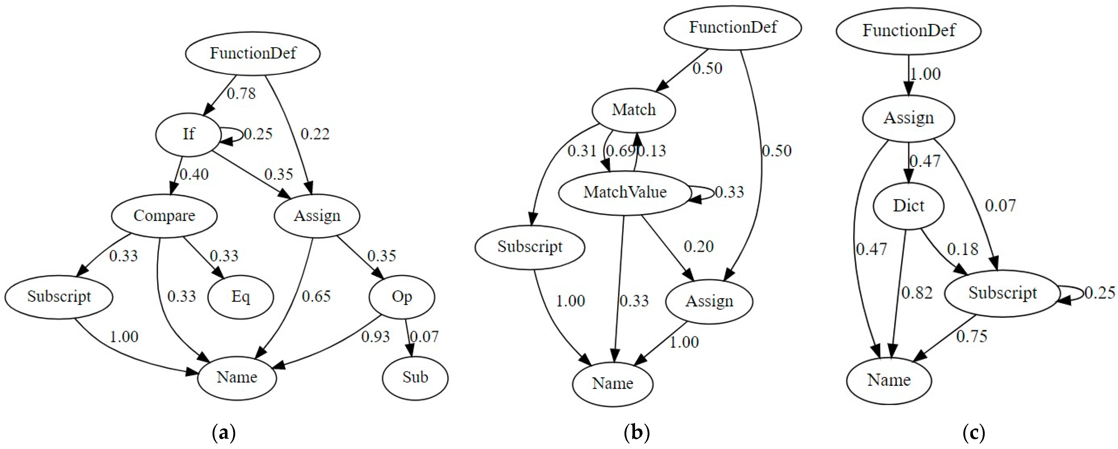
The examples of Markov chain state transition graphs obtained for programs that employ different approaches to solve different automatically generated tasks of type 6 (see Table 1, see Figure 1a) are shown in Figure 3.
While different program texts may contain different node types, the set H containing all different AST node types that occur in Markov chains in a particular dataset is preliminarily constructed. All weighted adjacency matrices are constructed based on the H set, and every weighted adjacency matrix belongs to H × H . The probabilities of transitions among node types that do not exist in a particular program text p i but exist in other program texts are set to zeros in the resulting weighted adjacency matrix.
In the final step, the weighted adjacency matrices of Markov chain state transition graphs are reshaped to vectors belonging to m , where m = H 2 . This way the mapping f : P m is implemented, where P denotes the set of program texts, and m is the dimensionality of a vector. Algorithm 1 summarizes the vectorization process of a dataset containing source codes of programs solving automatically generated tasks of a particular type (see Table 1).
Algorithm 1 Vectorization of a set of program texts based on Markov chains.
Input: P = p 1 , ,   p i , , p n -a set containing n program texts.
1.Define the set of Markov chain state transition graphs G = .
2.Define R =  {Import, Load, Store, alias, arguments, arg, Module, keyword}.
3.For each program text p i P  do:
4.  Construct an AST a i for p i using Python standard library (see Figure 2).
5.  Remove nodes belonging to the R set from a i .
6.  Replace nodes in a i according to Table 2.
7.  Construct Markov chain state transition graph g i for a i (see Figure 3).
8.   G G g i .
9.End loop.
10.Define the set H with all different node types existing in graphs from G .
11.Define the set of vector representations of program texts V = .
12.For each Markov chain state transition graph g i G  do:
13.  Construct an adjacency matrix m i H × H for the weighted graph g i .
14.  Reshape the m i matrix to vector v i m , where m = H 2 .
15.   V V v i .
16.End loop.
17.Return the set of vector representations of program texts V and the set H .
In the DTA analytics module, programs solving automatically generated tasks are vectorized all at once according to Algorithm 1, which only requires a set of program texts as input. After applying an unsupervised machine learning algorithm to the vectorized data, the DTA analytics module outputs a marked-up dataset. In that dataset, every i-th object is represented by a v i m vector, where m = H 2 , and H denotes the set containing all different AST node types that occur in all Markov chains obtained while vectorizing a particular set of program texts. Every i-th object has an associated class label y i Y , where Y is the set containing all possible classes discovered for a given dataset.
Algorithm 1 is only able to vectorize a set of program texts. However, vectorization of a single program text is required for unseen data classification. In order to vectorize a single program text p i P , Algorithm 2 is used. Algorithm 2 uses the H set while building a weighted adjacency matrix; the H set is obtained from Algorithm 1 and saved to disk before applying Algorithm 2.
Algorithm 2 Vectorization of a single program text p i based on Markov chains.
Input: p i -a program text,
H -a set with all different node types that exist in Markov chains of programs solving tasks of the same type as p i , this set is obtained by Algorithm 1.
1.Define R =  {Import, Load, Store, alias, arguments, arg, Module, keyword}.
2.Construct an AST a i for p i using Python standard library (see Figure 2).
3.Remove nodes belonging to the R set from a i .
4.Replace nodes in a i according to Table 2.
5.Construct Markov chain state transition graph g i for a i (see Figure 3).
6.Construct an adjacency matrix m i H × H for the weighted graph g i .
7.Reshape the m i matrix to vector v i m , where m = H 2 .
8.Return the vector v i representing the program text.
To sum up, the main difference between Algorithms 1 and 2 is that Algorithm 1 can only vectorize a set of program texts solving automatically generated tasks of a given type. This is particularly useful when applying a clustering algorithm to the whole dataset, with an intention to automatically discover the most common methods used by students while solving programming tasks of a given type. Algorithm 2, in contrast, can only be used to vectorize a single program text solving unique tasks of the same type, using the persisted H set that has been preliminarily obtained from Algorithm 1. Algorithm 2 is particularly useful when performing new data classification in real time, aiming to determine the solution method used in a newly submitted program text.

4. Program Text Classification

The DTA analytics module outputs marked-up datasets containing vector representations of program codes, and every vector has an associated class label. These datasets can be used to train classification algorithms that can be later used to classify new program texts submitted by students.
In a classification problem, a set of objects X = X L X T is given, where X L denotes the training set, X T denotes the testing set; a set of possible answers Y is given as well, and an unknown target function f : X Y , which maps the set of objects into the set of answers. The values of f are known for every object from the X set. The X L set is used while training a classifier, and the X T set is used while assessing classifier performance. Objects from the X set are represented as vectors and X = x 1 , , x i ,   x s , s denotes objects count in the dataset. Every j-th component of the i-th object x i = h i , 1 , , h i , j , , h i , n encodes j-th characteristic of the object, h i j , and x i n . The goal of a classification algorithm is to construct such mapping as a : X Y , that approximates the unknown target function f even on data unseen by a classifier.
In this paper we consider such classification algorithms as SVM, KNN, RF, and ELM. The implementations of SVM, KNN, and RF algorithms used in this research are based on the sklearn library [39]. ELM is implemented using the numpy library [40].

4.1. Support Vector Machine Classifier

The core idea of the SVM algorithm is that input vectors are nonlinearly mapped into a higher-dimensional space where a linear decision surface is constructed [12]. This algorithm was initially designed for binary classification. However, several methods exist that extend SVM to multi-class classification [22,41].
The two most common approaches are the “one-against-one” method and the “one-against-all” method. In the former approach, several binary SVM classifiers are constructed. Each classifier is trained using data from two classes, and the decisions of the classifiers are combined together. In the latter approach, each class is trained against the aggregate of all other classes. In this study the “one-against-one” approach for multi-class classification is used, which is implemented in the sklearn library [39].

4.2. K Nearest Neighbors Classifier

Neighbors-based classification does not attempt to construct a general model. Instead, it internally stores instances of training data, and the decision on which class to assign to an unseen sample is made based on a majority vote of the k nearest neighbors of a sample [14,39]. Nearest neighbor count k is a data-dependent hyperparameter of KNN, and the performance of this simple classification algorithm highly depends on k .

4.3. Random Forest Classifier

RF is an ensemble-based algorithm that fits a number of decision tree classifiers to training data [15,39]. The decision tree classifiers then consolidate their outcomes over a voting procedure. The most generally used collective strategies are bagging and boosting [42]. The hyperparameters of RF include the maximum number of decision trees in an ensemble, maximum decision tree depth, and the size of random subsets of features [39].

4.4. Extreme Learning Machine Classifier

Extreme learning machine (ELM) is a supervised machine learning algorithm proposed in [20]. ELMs originate from such algorithms as neural networks with random weights (NNRW) [43] and random vector functional link networks (RVFL) [44], and have been successfully applied to various real-world problems [22,23,24,26]. An ELM is a computationally inexpensive algorithm in comparison with neural networks trained with backpropagation or with evolutionary algorithms [45].
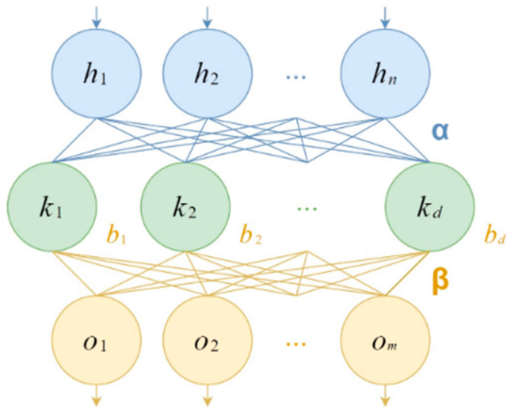
The structure of the ELM adopted for classification is shown in Figure 4. The weights of connections among neurons in ELM can be modeled as two matrices, α and β . Cells of the α matrix represent weights of connections among n input neurons h 1 , h 2 , , h n and d hidden neurons k 1 , k 2 , , k d , so α d × n . Cells of the α matrix are initialized randomly, as well as hidden layer biases b 1 , b 2 , , b d (see Figure 4).
The matrix β d × m containing the weights of connections among d hidden neurons k 1 , k 2 , , k d and m output neurons o 1 , o 2 , , o m is computed according to:
β = H Y L ,
where Y L s × m denotes a matrix containing one-hot encoded class labels for s objects from the training set X L that is represented as a matrix X L s × n , m denotes the dimensionality of s one-hot encoded class labels, m also equals to class count, n denotes the dimensionality of input vectors, n equals to input neurons count in ELM. H denotes the Moore–Penrose pseudoinverse [21] of the hidden layer output matrix H , the H matrix belongs to d × s , where s denotes objects count in X L , d denotes hidden neuron count, the hidden layer output matrix pseudoinverse H d × s is computed as:
H = H T H + γ I 1 H T ,
where H s × d is the hidden layer output matrix; H T d × s is the transpose of the hidden layer output matrix H ;   I d × d denotes the identity matrix; γ is the scalar regularization parameter, regularization is required in order to handle cases when the matrix being inverted is singular, and γ is one of the hyperparameters of the ELM algorithm.
The hidden layer output matrix H is computed according to:
H = σ X L α T + b ,
where X L s × n is the training set represented as a matrix and containing s rows, every row encodes an n -dimensional vector; α T n × d is the transpose of the α matrix containing weights of connections among n input and d hidden neurons, α d × n , the cells in α are randomly initialized and belong to 1 , 1 ; b s × d is a matrix containing hidden layer biases that is obtained by transforming the bias vector b = b 1 , b 2 , , b d belonging to d (see Figure 4) to a matrix belonging to s × d by mapping d into 1 × d , and then cloning the first row s times, the components of the bias vector b d are randomly initialized as well; σ is an infinitely differentiable [20] activation function that is applied to every cell of the hidden layer output matrix, sigmoid works best [45] in ELMs.
The sigmoid activation function is given by the following equation:
σ x = 1 1 e x
where x denotes the cell of the H s × d matrix before activation.
Input neuron count s depends on the considered classification or regression problem, hidden layer neuron count d is the hyperparameter of ELM, and output neuron count m is either set to 1 if a regression problem is considered, or is equal to the count of classes in a multi-class classification problem, where each class label is one-hot encoded.
The training process in ELM is described in Algorithm 3.
Algorithm 3 Extreme learning machine training.
Input: X L s × n -matrix of s rows encoding n -dimensional input vectors,
Y L s × m -matrix of s rows encoding m -dimensional output vectors,
γ -regularization parameter,
d -hidden neuron count,
σ -hidden layer activation function.
1.Initialize the weights α d × n with uniformly distributed random numbers.
2.Initialize the biases b d with uniformly distributed random numbers.
3.Compute  b s × d by cloning b d   s times.
4.Compute hidden layer output matrix H = σ X L α T + b .
5.Initialize the identity matrix I d × d .
6.Compute pseudoinverse H = H T H + γ I 1 H T .
7.Compute the weights β d × m according to β = H Y L .
8.Return input weights α d × n , biases b d , output weights β d × m .
The series of steps performed while making predictions in ELM is described in Algorithm 4. Such ELM parameters as regularization coefficient γ and hidden layer size d are typically tuned using grid search.
Algorithm 4 Extreme learning machine predictions.
Input: X T s × n -matrix of s rows encoding n -dimensional input vectors,
γ -regularization parameter,
d -hidden neuron count,
σ -hidden layer activation function,
α d × n -input weights,
b d -hidden layer biases,
β d × m -output weights.
1.Compute  b s × d by cloning b d   s times.
2.Compute hidden layer output matrix H = σ X T α T + b .
3.Compute the output matrix Y T = H β belonging to s × m .
4.Return the Y T matrix of s rows encoding m -dimensional output vectors.

4.5. Multi-Class Classification Metrics

The most commonly used classification metrics are Accuracy, Precision, Recall, and F1 score [46]. Precision for binary classification is computed according to:
P r e c i s i o n = T P T P + F P ,
where T P denotes true positive elements—such elements that have been labeled as positive by a classification model and they are actually positive; F P denotes false positive elements—such elements that have been labeled as positive, but they are negative.
Recall for binary classification is computed according to:
R e c a l l = T P T P + F N ,
where T P denotes true positive elements; F N denotes false negative elements—such elements that have been labeled as negative by a classifier, but they are actually positive.
F1 score is the harmonic mean of Precision (5) and Recall (6) scores, given by:
F 1   s c o r e = 2 P r e c i s i o n     R e c a l l P r e c i s i o n   +   R e c a l l .
For a problem of data classification into K classes, accuracy, Precision, Recall, and F1 score metrics are computed for every k-th class label separately, assuming elements with the k-th class label as positive and elements with any other class label as negative. Next, either a weighted or unweighted average is computed for scores for every class label.
Unweighted averages of Precision (5), Recall (6), F1 score (7) are also known as macro averages [46]. Macro Precision (5) for multi-class classification is given by:
M a c r o P r e c i s i o n = 1 K k = 1 K T P k T P k + F P k ,
where k denotes class label index; T P k denotes true positive elements for the k-th class label; F P k denotes false positive elements for the k-th class label, K denotes total count of classes in a multi-class classification problem.
Macro Recall (6) for multi-class classification is given by:
M a c r o R e c a l l = 1 K k = 1 K T P k T P k + F N k ,
where k denotes class label index; T P k denotes true positive elements for the k-th class label; F N k denotes false negative elements for the k-th class label, K denotes total count of classes in a multi-class classification problem.
Finally, the Macro F1 score that is the harmonic mean for (8) and (9) is given by:
M a c r o   F 1   s c o r e = 2 M a c r o P r e c i s i o n     M a c r o R e c a l l M a c r o P r e c i s i o n   +   M a c r o R e c a l l .
Such metrics as (8), (9), and (10) are useful when searching for a classifier without bias towards classes that occur in a dataset most frequently.
Finally, the Accuracy score for multi-class classification is the sum of true positive and true negative elements of each class k divided by class count K. The formula for the Accuracy score is as follows:
A c c u r a c y = 1 K k = 1 K T P k + T N k T P k + T N k + F P k + F N k ,
where k denotes class label index, T P k denotes true positive elements for the k-th class label; T N k denotes true negative elements for the k-th class label-such elements that have been correctly labeled as negative; F P k denotes false positive elements; F N k denotes false negative elements for the k-th class label, K denotes total count of classes in a multi-class classification problem.

4.6. Biology-Inspired Algorithms-Enhanced Extreme Learning Machines

Preliminary experiments have shown that the ELM algorithm is the fastest multi-class classification technique among the considered ones in terms of prediction making, and one of the fastest techniques in terms of model training, hence we considered an ELM fine-tuning technique that only slightly slowed down the classifier development process, but allowed us to obtain highly accurate and fast ELM classification models. Notably, other discussed classifiers such as SVM or KNN could also be either hybridized [47] or improved with fine-tuning methods [48,49].
Random initialization of weights of connections among input and hidden neurons α and hidden layer biases b does not guarantee that the optimal ELM structure is obtained during training (see Algorithm 3). In order to overcome this issue, researchers often apply biology-inspired algorithms to input weights and hidden biases tuning [24,25,26]. In [25], the authors use the particle swarm optimization (PSO) algorithm in order to improve the accuracy of ELM applied to short-term traffic flow forecasting. In [26], the authors fine-tune ELM models using the genetic algorithm (GA). In [24], the authors compare the performance of GA, PSO, and fish school search (FSS) optimization algorithms applied to input weights and biases tuning of ELMs solving regression problems. The FSS algorithm with exponential step decay (ETFSS) [50] showed the best performance.
In this paper, we apply the differential evolution (DE) [29] algorithm and the FSS algorithm with exponential step decay (ETFSS) [50] to input weights and hidden biases fine-tuning of ELMs used for program text classification. The Macro F1-score (10) is used as a fitness function. In order to enhance the generalization capabilities of ELM, the Macro F1 score (10) is obtained from test data that is not used during ELM training according to Algorithm 3. When optimizing the input weights α d × n , where d denotes hidden neuron count and n denotes the dimensionality of input vectors, and biases b d , every l-th agent in a biology-inspired algorithm is encoded as a real vector α 11 l , α 12 l , , α 1 n l , α 21 l , α 22 l , , α 2 n l , , α d 1 l , α d 2 l , , α d n l , b 1 l , b 2 l , , b d l [24,25].

5. Numerical Experiment

The experiments were conducted using 11 datasets containing program texts solving automatically generated tasks of 11 different types (see Table 1). The program texts were submitted by students to the DTA system and accepted by the DTA core task checker. Every dataset was preliminary vectorized using Algorithm 1. Every dataset was split into training and testing parts using the stratified split strategy available in sklearn [39]. The sizes of training and testing datasets are listed in Table 3, as well as class counts.
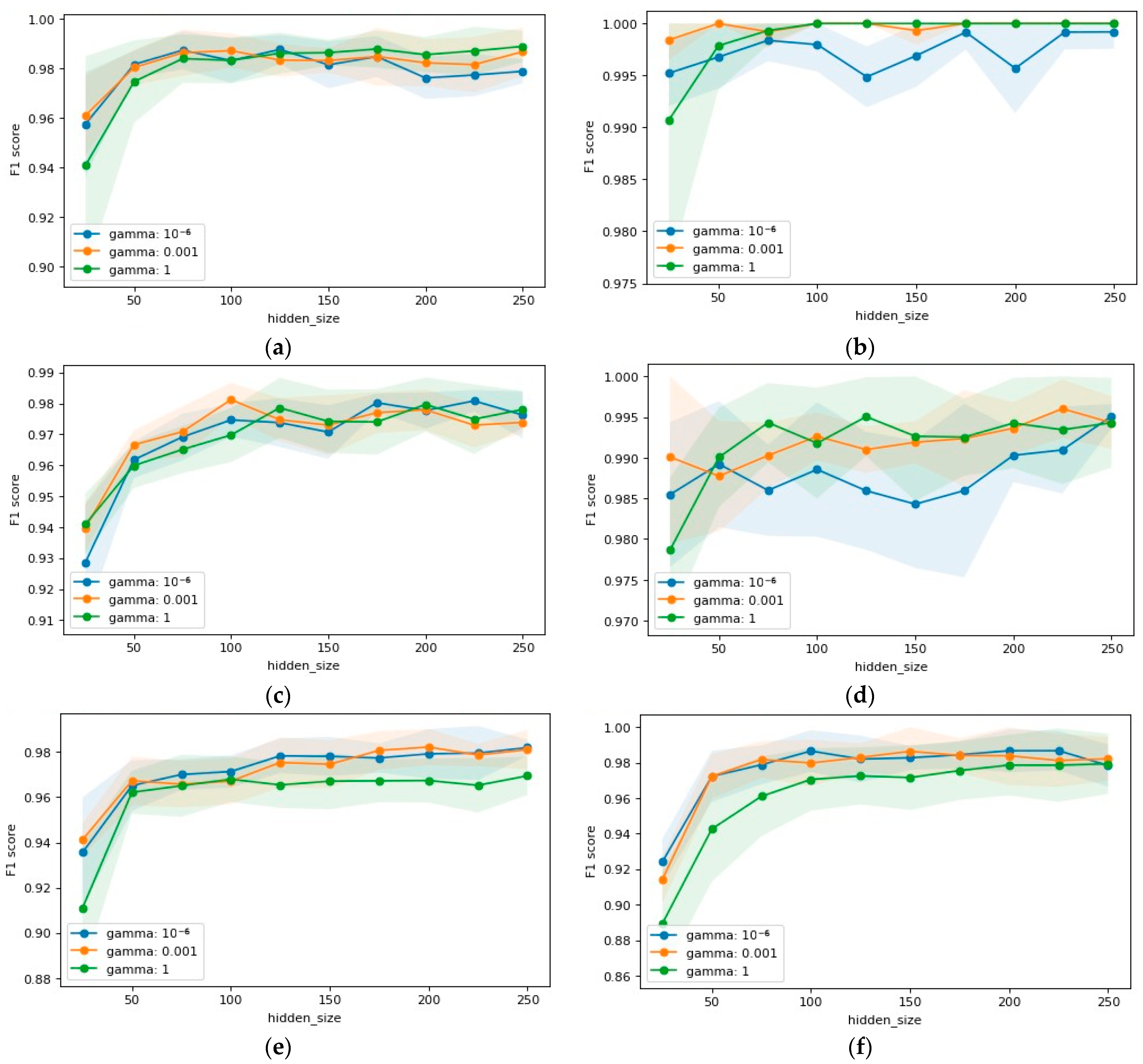
Vectors obtained using Algorithm 1 were passed to SVM, RF, KNN, and ELM classifiers. The hyperparameters of the classifiers were estimated on full datasets using a grid search [39] maximizing the Macro F1 score (10). The best parameters are listed in Table 4. The process of the regularization parameter γ and hidden neuron count d selection for ELMs is shown in Figure 5 for six of the most complex task types with the most diverse solutions.
According to Figure 5, ELM performance depends on the combination of γ and d , so these parameters should be tuned depending on the considered problem. The comparison of the considered SVM, RF, KNN, and ELM algorithms is provided in Table 5.
According to Table 5, ELM is the fastest classification algorithm among the considered ones. RF appeared to be the slowest algorithm due to its ensemble-based nature; however, it produces easily interpretable results modeled as decision trees. The performance of SVM heavily depends on the kernel function used: linear kernel is faster than RBF (see Table 4 and Table 5), however, ELM trains and predicts faster even when compared to linear SVM models. Even without additional tuning, ELM showed the best accuracy comparing to all other algorithms in two classification problems, and in one showed the same accuracy as SVM and KNN. KNN outperformed all algorithms in one of the classification problems, while in seven problems SVM showed the best accuracy.
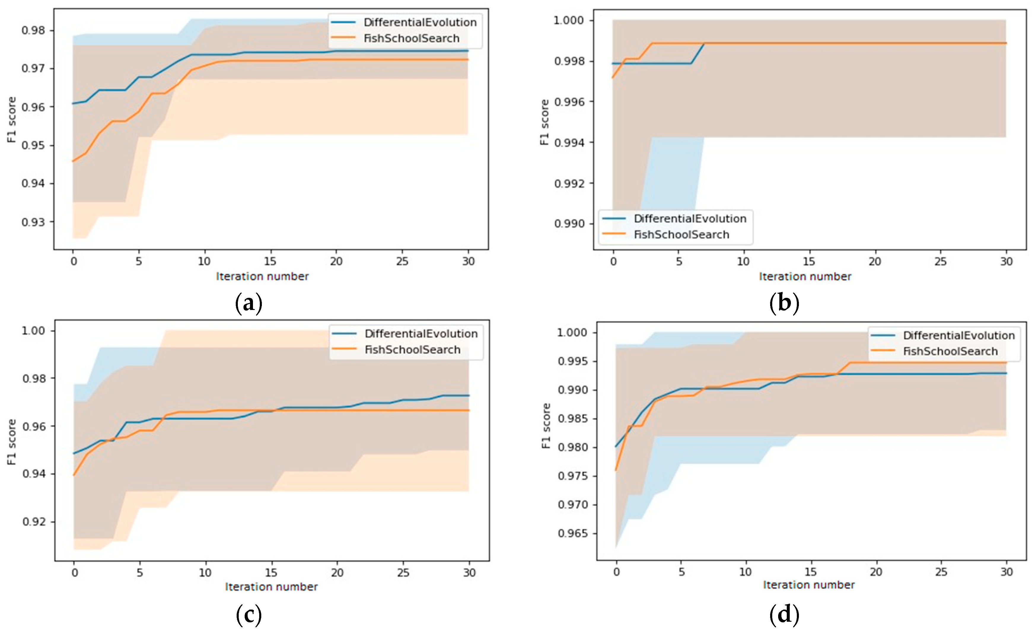
Aiming to stabilize and further enhance the performance of the fastest classification algorithm, we applied differential evolution (DE) [29] and fish school search with exponential step decay (ETFSS) [50] to ELM input weights and hidden biases fine-tuning by maximizing the Macro F1 score (10). The reasoning behind choosing these algorithms is described in Section 4.6. The experimentally selected parameters of the considered biology-inspired algorithms are listed in Table 6. The plots illustrating the convergence of the DE and ETFSS algorithms improving ELM performance in tasks with most diverse solutions are shown in Figure 6. The comparison of ELM with ELM models fine-tuned with DE (DELM) and with ELM models fine-tuned with ETFSS (FELM) is shown in Table 7.
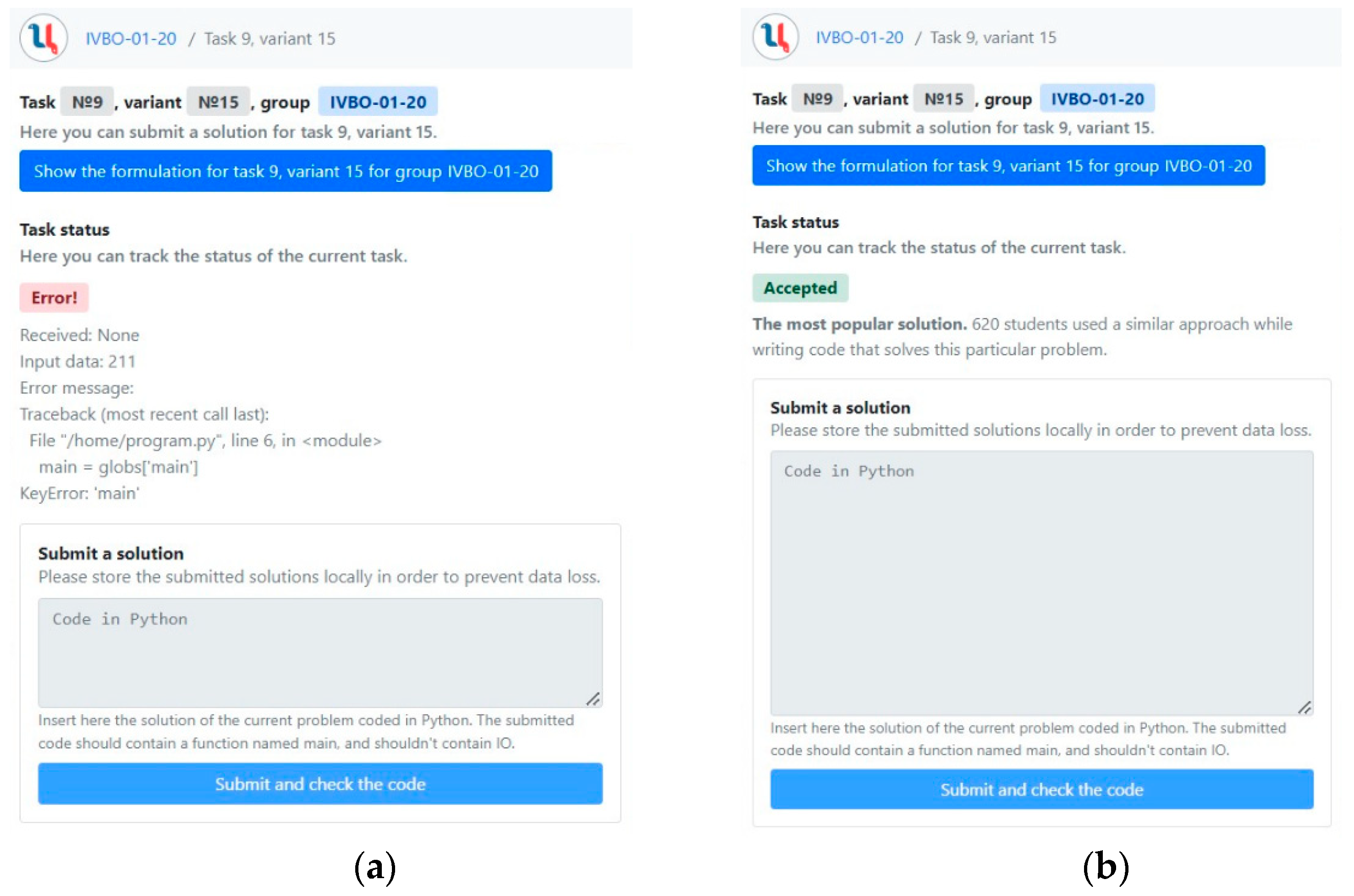
According to Figure 6 and Table 7, the biology-inspired algorithms with small iteration limit and small agent count show similar performance, and are able to stabilize ELM and improve the accuracy of the resulting model up to 100% in many of the considered multi-class classification problems. At the cost of time losses during the training phase, biology-inspired algorithms successfully automated the development of very accurate and fast ELM-based classifiers. The most accurate ELM-based classifiers evolved with the DE and ETFSS algorithms were incorporated into the DTA system and enabled real-time analysis of program texts submitted by students (see Figure 7b).

6. Discussion

In the research presented in this paper, we consider the classification problem of program texts solving automatically generated programming exercises of 11 different types (see Table 1). The programming exercises were generated by the Digital Teaching Assistant (DTA) system [9,10], which automates the massive Python programming course at MIREA-Russian Technological University. The solutions for the exercises were submitted to DTA by students using a web-based user interface [9].
The DTA system includes an analytics module used by teachers for the analysis of program texts submitted by students by the end of semester. The aim of such an analysis is to discover approaches used by students when solving the automatically generated tasks of different types generated by the DTA core module [6]. The analytics module is based on an unsupervised machine learning technique and preliminary transforms program texts into vectors according to Algorithm 1. The transformation algorithm constructs an AST (see Figure 2) for every program and uses intermediate program text representation based on Markov chain state transition graph for an AST (see Figure 3). After applying an unsupervised machine learning technique, the DTA analytics module outputs a marked-up dataset where program texts are represented as vectors. Every vector in such a dataset has an assigned class label indicating the number of the approach used by a student while solving a unique automatically generated task.
The marked-up datasets obtained from the DTA analytics module are then passed to the classifiers considered in this research, namely, SVM, KNN, RF, and ELM. The implementations for SVM, KNN, and RF classifiers were borrowed from the sklearn library [39], and the ELM-based classifier was implemented according to Algorithms 3 and 4 using numpy [40]. New program texts that were not preliminarily transformed into vectors by the DTA analytics module were vectorized according to Algorithm 2 (see Section 3) before being passed to a classifier. In order to estimate the performance of the considered multi-class classifiers, such metrics as Macro Precision (8), Macro Recall (9), and Macro F1 score (10) were used. The hyperparameters for each of the considered algorithms were tuned using a grid search [39]. The chosen parameters for most accurate classifiers of each type for different task types are listed in Table 4.
The results of the experimental run (see Table 5) indicate that ELM is the least computationally expensive algorithm among the considered ones. The performance of ELM depends on the chosen regularization parameter value, hidden neuron count (see Figure 5), and the input weights and hidden biases initialization. The weights and biases are initialized randomly in the original algorithm. Even without additional input weights and hidden biases tuning, commonly applied by researchers and practitioners [24,25,26], ELM outperformed other classification algorithms in two problems in terms of accuracy (see Table 5). After applying differential evolution (DE) and fish school search with exponential step decay (ETFSS) to input weights and hidden biases tuning, the accuracy of ELM considerably improved (Table 7) at the cost of time losses during training.
The most accurate ELM-based classifiers obtained with biology-inspired algorithms (see Table 7 and Figure 6) were incorporated into the DTA system for real-time analysis of student submissions. The sample web-based UI of the DTA web app [9] is shown in Figure 7. The sample classifier decision is shown in Figure 7b. Such classifiers also enable real-time analysis of student submissions by teachers, allowing programming instructors to discover the most common approaches used by students while solving automatically generated programming exercises during the semester. This allows filling the gaps in students’ knowledge by explaining the least frequently used language features of the Python programming language.
Future work could focus on building a system of achievements for improving the learning motivation [11] in the DTA digital environment (see Figure 7b) by suggesting students discover all possible approaches to solving a programming exercise of a particular type on their own. Additionally, further research could focus on performance investigation of modified and improved versions of the SVM [49] and KNN [48] algorithms, as well as their hybridized versions [47], ELMs with explicitly computed input weights [51], neural networks [52], and transformers [53], aiming to further enhance classification accuracy and reduce computational overhead when making class label predictions.

Author Contributions

Conceptualization, L.A.D. and A.V.G.; guidance, supervision, validation, L.A.D.; software, resources, visualization, testing, A.V.G.; original draft preparation, L.A.D. and A.V.G. All authors have read and agreed to the published version of the manuscript.

Funding

This research received no external funding.

Data Availability Statement

Not applicable.

Conflicts of Interest

The authors declare no conflict of interest.

References

  1. Moussiades, L.; Vakali, A. PDetect: A clustering approach for detecting plagiarism in source code datasets. Comput. J. 2005, 48, 651–661. [Google Scholar] [CrossRef]
  2. Kustanto, C.; Liem, I. Automatic Source Code Plagiarism Detection. In Proceedings of the 2009 10th ACIS International Conference on Software Engineering, Artificial Intelligences, Networking and Parallel/Distributed Computing, Daegu, Korea, 27–29 May 2009; IEEE: Pistacaway, NJ, USA, 2009; pp. 481–486. [Google Scholar]
  3. Jiang, L.; Misherghi, G.; Su, Z.; Glondu, S. Deckard: Scalable and Accurate Tree-Based Detection of Code Clones. In Proceedings of the 29-th International Conference on Software Engineering (ICSE’07), Minneapolis, MN, USA, 20–26 May 2007; IEEE: Pistacaway, NJ, USA, 2007; pp. 96–105. [Google Scholar]
  4. Chilowicz, M.; Duris, E.; Roussel, G. Syntax Tree Fingerprinting for Source Code Similarity Detection. In Proceedings of the 2009 IEEE 17th International Conference on Program Comprehension, Vancouver, BC, Canada, 17–19 May 2009; IEEE: Pistacaway, NJ, USA, 2009; pp. 243–247. [Google Scholar]
  5. Yasaswi, J.; Kailash, S.; Chilupuri, A.; Purini, S.; Jawahar, C.V. Unsupervised Learning-Based Approach for Plagiarism Detection in Programming Assignments. In Proceedings of the 10th Innovations in Software Engineering Conference, Jaipur, India, 5–7 February 2017; Association for Computing Machinery: New York, NY, USA, 2017; pp. 117–121. [Google Scholar]
  6. Sovietov, P. Automatic Generation of Programming Exercises. In Proceedings of the 2021 1st International Conference on Technology Enhanced Learning in Higher Education (TELE), Lipetsk, Russia, 24–25 June 2021; IEEE: Pistacaway, NJ, USA, 2021; pp. 111–114. [Google Scholar]
  7. Wakatani, A.; Maeda, T. Automatic Generation of Programming Exercises for Learning Programming Language. In Proceedings of the 2015 IEEE/ACIS 14th International Conference on Computer and Information Science (ICIS), Las Vegas, NV, USA, 28 June–1 July 2015; IEEE: Pistacaway, NJ, USA, 2015; pp. 461–465. [Google Scholar]
  8. Staubitz, T.; Klement, H.; Renz, J.; Teusner, R.; Meinel, C. Towards Practical Programming Exercises and Automated Assessment in Massive Open Online Courses. In Proceedings of the 2015 IEEE International Conference on Teaching, Assessment, and Learning for Engineering (TALE), Zhuhai, China, 10–12 December 2015; IEEE: Pistacaway, NJ, USA, 2015; pp. 23–30. [Google Scholar]
  9. Sovietov, P.N.; Gorchakov, A.V. Digital Teaching Assistant for the Python Programming Course. In Proceedings of the 2022 2nd International Conference on Technology Enhanced Learning in Higher Education (TELE), Lipetsk, Russia, 26–27 May 2022; IEEE: Pistacaway, NJ, USA, 2022; pp. 272–276. [Google Scholar]
  10. Andrianova, E.G.; Demidova, L.A.; Sovetov, P.N. Pedagogical design of a digital teaching assistant in massive professional training for the digital economy. Russ. Technol. J. 2022, 10, 7–23. [Google Scholar] [CrossRef]
  11. Su, C.H.; Cheng, C.H. A mobile gamification learning system for improving the learning motivation and achievements. J. Comput. Assist. Learn. 2015, 31, 268–286. [Google Scholar] [CrossRef]
  12. Cortes, C.; Vapnik, V. Support-vector Networks. Mach. Learn. 1995, 20, 273–297. [Google Scholar] [CrossRef]
  13. Altman, N.S. An introduction to kernel and nearest-neighbor nonparametric regression. Am. Stat. 1992, 46, 175–185. [Google Scholar]
  14. Wu, Y.; Ianakiev, K.; Govindaraju, V. Improved K-nearest neighbor classification. Pattern Recognit. 2002, 35, 2311–2318. [Google Scholar] [CrossRef]
  15. Ho, T.K. Random Decision Forests. In Proceedings of the 3rd International Conference on Document Analysis and Recognition, Montreal, QC, Canada, 14–16 August 1995; IEEE: Pistacaway, NJ, USA, 1995; pp. 278–282. [Google Scholar]
  16. Rosenblatt, F. The perceptron: A probabilistic model for information storage and organization in the brain. Psychol. Rev. 1958, 65, 386–408. [Google Scholar] [CrossRef]
  17. Ruder, S. An overview of gradient descent optimization algorithms. arXiv 2016, arXiv:1609.04747. [Google Scholar]
  18. Chen, N.; Xiong, C.; Du, W.; Wang, C.; Lin, X.; Chen, Z. An improved genetic algorithm coupling a back-propagation neural network model (IGA-BPNN) for water-level predictions. Water 2019, 11, 1795. [Google Scholar] [CrossRef]
  19. Demidova, L.A.; Gorchakov, A.V. A Study of Biology-inspired Algorithms Applied to Long Short-Term Memory Network Training for Time Series Forecasting. In Proceedings of the 2021 3rd International Conference on Control Systems, Mathematical Modeling, Automation and Energy Efficiency (SUMMA), Lipetsk, Russia, 10–12 November 2021; IEEE: Pistacaway, NJ, USA, 2021; pp. 473–478. [Google Scholar]
  20. Huang, G.B.; Zhu, Q.Y.; Siew, C.K. Extreme Learning machine: Theory and applications. Neurocomputing 2006, 70, 489–501. [Google Scholar] [CrossRef]
  21. Rao, C.R. Generalized Inverse of a Matrix and its Applications. In Proceedings of the Sixth Berkeley Symposium on Mathematical Statistics and Probability, Theory of Statistics, Berkeley, CA, USA, 21 June–18 July 1970; University of California Press: Berkeley, CA, USA, 1972; pp. 601–620. [Google Scholar]
  22. Cheng, C.; Tay, W.P.; Huang, G.B. Extreme Learning Machines for Intrusion Detection. In Proceedings of the 2012 International Joint Conference on Neural Networks (IJCNN), Brisbane, Australia, 10–15 June 2012; IEEE: Pistacaway, NJ, USA, 2012; pp. 1–8. [Google Scholar]
  23. Liu, Y.; Loh, H.T.; Tor, S.B. Comparison of Extreme Learning Machine with Support Vector Machine for Text Classification. In Proceedings of the International Conference on Industrial, Engineering and Other Applications of Applied Intelligent Systems, Innovations in Applied Artificial Intelligence, Bari, Italy, 22–24 June 2005; Springer: Berlin, Germany, 2005; pp. 390–399. [Google Scholar]
  24. Demidova, L.A.; Gorchakov, A.V. Application of bioinspired global optimization algorithms to the improvement of the prediction accuracy of compact extreme learning machines. Russ. Technol. J. 2022, 10, 59–74. [Google Scholar] [CrossRef]
  25. Cai, W.; Yang, J.; Yu, Y.; Song, Y.; Zhou, T.; Qin, J. PSO-ELM: A hybrid learning model for short-term traffic flow forecasting. IEEE Access 2020, 8, 6505–6514. [Google Scholar] [CrossRef]
  26. Song, S.; Wang, Y.; Lin, X.; Huang, Q. Study on GA-based Training Algorithm for Extreme Learning Machine. In Proceedings of the 2015 7th International Conference on Intelligent Human-Machine Systems and Cybernetics, Hangzhou, China, 26–27 August 2015; IEEE: Pistacaway, NJ, USA, 2015; Volume 2, pp. 132–135. [Google Scholar]
  27. Eremeev, A.V. A genetic algorithm with tournament selection as a local search method. J. Appl. Ind. Math 2012, 6, 286–294. [Google Scholar] [CrossRef]
  28. Kennedy, J.; Eberhart, R. Particle swarm optimization. In Proceedings of the ICNN’95-International Conference on Neural Networks, Perth, WA, Australia, 27 November–1 December 1995; Volume 4, pp. 1942–1948. [Google Scholar]
  29. Storn, R.; Price, K. Differential evolution—A simple and efficient heuristic for global optimization over continuous spaces. J. Glob. Optim. 1997, 11, 341–359. [Google Scholar] [CrossRef]
  30. Monteiro, R.P.; Verçosa, L.F.V.; Bastos-Filho, C.J.A. Improving the performance of the fish school search algorithm. Int. J. Swarm Intell. Res. 2018, 9, 21–46. [Google Scholar] [CrossRef]
  31. Stanovov, V.; Akhmedova, S.; Semenkin, E. Neuroevolution of augmented topologies with difference-based mutation. IOP Conf. Ser. Mater. Sci. Eng. 2021, 1047, 012075. [Google Scholar] [CrossRef]
  32. Ananthi, J.; Ranganathan, V.; Sowmya, B. Structure Optimization Using Bee and Fish School Algorithm for Mobility Prediction. Middle-East J. Sci. Res 2016, 24, 229–235. [Google Scholar]
  33. Prosvirin, A.; Duong, B.P.; Kim, J.M. SVM Hyperparameter Optimization Using a Genetic Algorithm for Rub-Impact Fault Diagnosis. Adv. Comput. Commun. Comput. Sci. 2019, 924, 155–165. [Google Scholar]
  34. Baioletti, M.; Di Bari, G.; Milani, A.; Poggioni, V. Differential Evolution for Neural Networks Optimization. Mathematics 2020, 8, 69. [Google Scholar] [CrossRef]
  35. Gilda, S. Source Code Classification using Neural Networks. In Proceedings of the 2017 14th International Joint Conference on Computer Science and Software Engineering (JCSSE), Nakhon Si Thammarat, Thailand, 12–14 July 2017; IEEE: Pistacaway, NJ, USA, 2017; pp. 1–6. [Google Scholar]
  36. Alon, U.; Zilberstein, M.; Levy, O.; Yahav, E. code2vec: Learning Distributed Representations of Code. In Proceedings of the ACM on Programming Languages, Athens, Greece, 21–22 October 2019; Association for Computing Machinery: New York, NY, USA, 2019; Volume 3, pp. 1–29. [Google Scholar]
  37. Gansner, E.R.; North, S.C. An Open Graph Visualization System and Its Applications to Software Engineering. Softw. Pract. Exp. 2000, 30, 1203–1233. [Google Scholar] [CrossRef]
  38. Berthiaux, H.; Mizonov, V. Applications of Markov chains in particulate process engineering: A review. Can. J. Chem. Eng. 2004, 82, 1143–1168. [Google Scholar] [CrossRef]
  39. Pedregosa, F.; Varoquaux, G.; Gramfort, A.; Michel, V.; Thirion, B.; Grisel, O.; Blondel, M.; Prettenhofer, P.; Weiss, R.; Dubourg, V.; et al. Scikit-learn: Machine learning in Python. J. Mach. Learn. Res. 2011, 12, 2825–2830. [Google Scholar]
  40. Harris, C.R.; Millman, K.J.; van der Walt, S.J.; Gommers, R.; Virtanen, P.; Cournapeau, D.; Wieser, E.; Taylor, J.; Berg, S.; Smith, N.J.; et al. Array programming with NumPy. Nature 2020, 585, 357–362. [Google Scholar] [CrossRef] [PubMed]
  41. Hsu, C.-W.; Lin, C.-J. A comparison of methods for multiclass support vector machines. IEEE Trans. Neural Netw. 2002, 13, 415–425. [Google Scholar]
  42. Parmar, A.; Katariya, R.; Patel, V. A Review on Random Forest: An Ensemble Classifier. In Proceedings of the International Conference on Intelligent Data Communication Technologies and Internet of Things, Coimbatore, India, 7–8 August 2018; Springer: Cham, Switzerland, 2018; pp. 758–763. [Google Scholar]
  43. Schmidt, W.F.; Kraaijveld, M.A.; Duin, R.P. W Feedforward Neural Networks with Random Weights. In Proceedings of the 11th IAPR International Conference on Pattern Recognition, Pattern Recognition Methodology and Systems, The Hague, The Netherlands, 30 August–3 September 1992; IEEE: Pistacaway, NJ, USA, 1992; Volume 2, pp. 1–4. [Google Scholar]
  44. Pao, Y.H.; Takefji, Y. Functional-link net computing: Theory, system architecture, and functionalities. Computer 1992, 25, 76–79. [Google Scholar] [CrossRef]
  45. Cao, W.; Gao, J.; Ming, Z.; Cai, S. Some tricks in parameter selection for extreme learning machine. IOP Conf. Ser. Mater. Sci. Eng. 2017, 261, 012002. [Google Scholar] [CrossRef]
  46. Grandini, M.; Bagli, E.; Visani, G. Metrics for Multi-class Classification: An Overview. arXiv 2020, arXiv:2008.05756. [Google Scholar]
  47. Demidova, L.A. Two-Stage Hybrid Data Classifiers Based on SVM and kNN Algorithms. Symmetry 2021, 13, 615. [Google Scholar] [CrossRef]
  48. Liu, G.; Zhao, H.; Fan, F.; Liu, G.; Xu, Q.; Nazir, S. An Enhanced Intrusion Detection Model Based on Improved kNN in WSNs. Sensors 2022, 22, 1407. [Google Scholar] [CrossRef]
  49. Razaque, A.; Ben Haj Frej, M.; Almi’ani, M.; Alotaibi, M.; Alotaibi, B. Improved Support Vector Machine Enabled Radial Basis Function and Linear Variants for Remote Sensing Image Classification. Sensors 2021, 21, 4431. [Google Scholar] [CrossRef]
  50. Demidova, L.A.; Gorchakov, A.V. A Study of Chaotic Maps Producing Symmetric Distributions in the Fish School Search Optimization Algorithm with Exponential Step Decay. Symmetry 2020, 12, 784. [Google Scholar] [CrossRef]
  51. Tapson, J.; Chazal, P.D.; Schaik, A.V. Explicit Computation of Input Weights in Extreme Learning Machines. In Proceedings of the ELM-2014, Singapore, 8–10 December 2014; Springer: Cham, Switzerland, 2014; Volume 1, pp. 41–49. [Google Scholar]
  52. Cao, Z.; Chu, Z.; Liu, D.; Chen, Y. A Vector-Based Representation to Enhance Head Pose Estimation. In Proceedings of the IEEE/CVF Winter Conference on Applications of Computer Vision, Hawaii, HI, USA, 19–25 June 2021; IEEE: Pistacaway, NJ, USA, 2021; pp. 1188–1197. [Google Scholar]
  53. Wang, Q.; Fang, Y.; Ravula, A.; Feng, F.; Quan, X.; Liu, D. WebFormer: The Web-Page Transformer for Structure Information Extraction. In Proceedings of the ACM Web Conference 2022, Lyon, France, 25–29 April 2022; Association for Computing Machinery: New York, NY, USA, 2022; pp. 3124–3133. [Google Scholar]
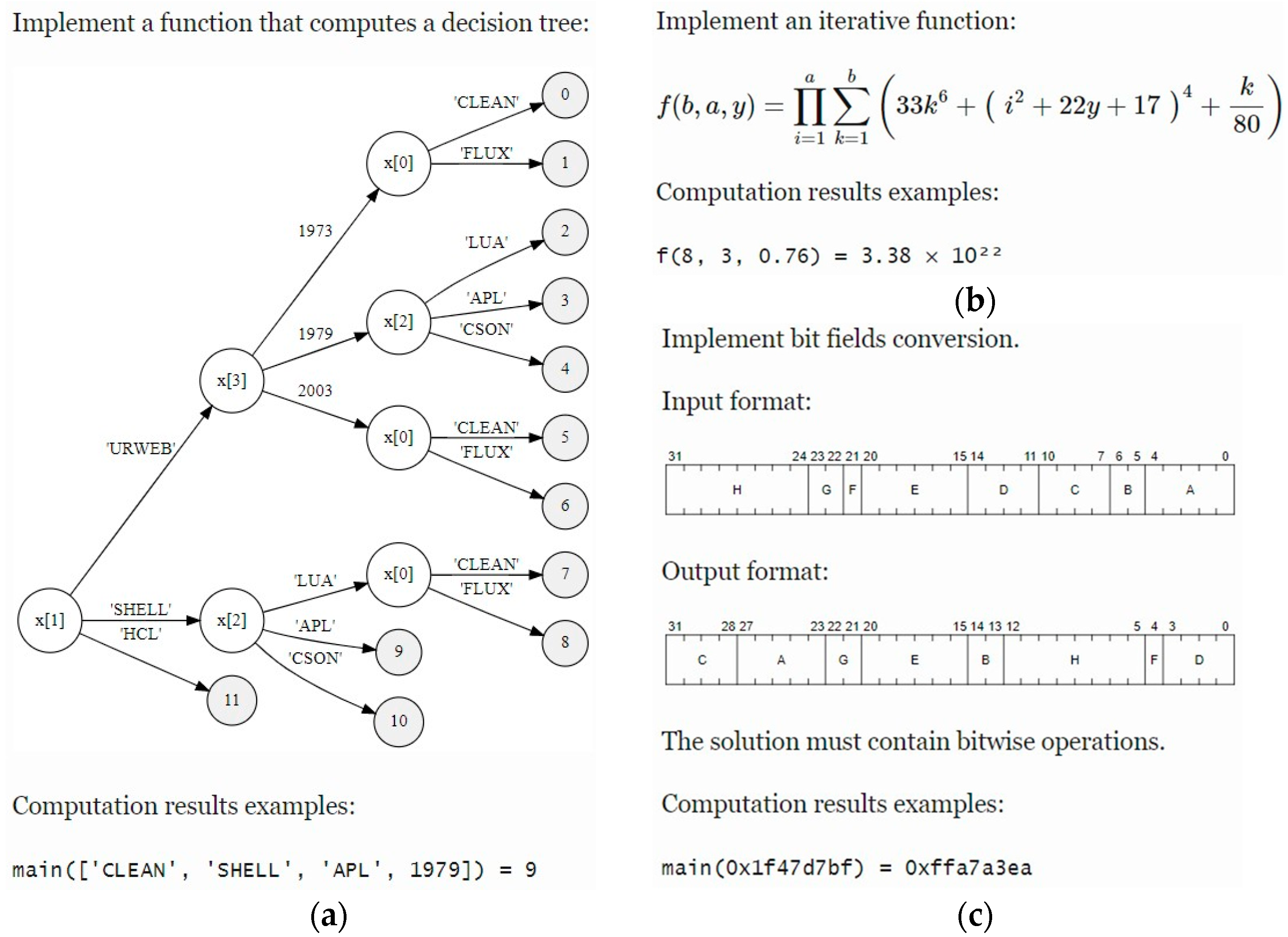
Figure 1. Examples of formulations for unique programming tasks of various types (see Table 1) automatically generated [6] by the DTA system [9,10]: (a) implement a decision tree, (b) implement an iterative function, (c) implement bit fields conversion.
Algorithms 15 00329 g001
Figure 2. AST of a program that solves one of the automatically generated tasks of type 6 (see Table 1, see Figure 1a) using a pattern matching-based approach, after applying AST transformations during program text vectorization in DTA.
Algorithms 15 00329 g002
Figure 3. Markov chain state transition graphs for programs that employ different approaches to solve automatically generated tasks of type 6 (see Table 1, see Figure 1a): (a) solution using conditional operators; (b) solution using pattern matching; (c) solution using dictionaries.
Algorithms 15 00329 g003
Figure 4. The structure of an extreme learning machine.
Algorithms 15 00329 g004
Figure 5. ELM (see Algorithms 3 and 4) hyperparameter selection for classification of program texts solving automatically generated tasks of various types (see Table 1): (a) task of type 6; (b) task of type 7; (c) task of type 8; (d) task of type 9; (e) task of type 10; (f) task of type 11.
Algorithms 15 00329 g005
Figure 6. Convergence of the considered biology-inspired algorithms DE and ETFSS optimizing the macro f1 score (10) in testing part of the dataset containing program texts solving automatically generated tasks of various types (see Table 1): (a) type 8; (b) type 9; (c) type 10; (d) type 11.
Algorithms 15 00329 g006
Figure 7. DTA [9,10] web-based UI: (a) displaying an error message, (b) displaying real-time program text analysis results obtained from ELM fine-tuned with biology-inspired algorithms.
Algorithms 15 00329 g007
Table 1. Brief descriptions of programming exercise types available in DTA.
Task TypeBrief Description
1Implement a function
2Implement a piecewise function
3Implement an iterative function
4Implement a recurrent function
5Implement a function that operates on vectors
6Implement a function that computes a decision tree
7Implement bit fields conversion
8Implement text format parsing
9Implement a Mealy finite-state machine
10Implement tabular data transformation
11Implement binary data format parsing
Table 2. Replacements of AST node types while building Markov chain state transition graphs.
Replacements for 1–11 Task TypesReplacements for 6–11 Task Types
Replaceable VertexReplacementReplaceable VertexReplacement
Constant, AttributeNameList, Tuple, SetList
BoolOp, Call, UnaryOp, BinOpOpLambda, JoinedStr, FormattedValueName
Lt, LtELessPass, Break, ContinueNone
Gt, GtEGreaterExceptHandlerTry
AugAssign, AnAssignAssignIfExpIf
match_case, MatchStar, MatchAs, MatchOr, MatchSingleton, MatchSequence, MatchMapping, MatchClassMatchValueFor, While, ListComp, SetComp, DictComp, GeneratorExp, comprehensionLoop
UAddAdd
USubSub
Table 3. Brief information about datasets of programs solving tasks of different types.
Task TypeTraining Dataset SizeTesting Dataset SizeClass Count
19183944
29033874
38473643
48303565
58633705
68623708
78713746
88603695
98613708
108473645
1182135314
Table 4. Parameters selected for SVM, RF, KNN, and ELM using grid search maximizing (10).
Task
Type
RFSVMKNNELM
DepthTreesCKernelKWeights γ Neurons
110401Linear3Uniform10−625
22012010RBF3Uniform0.001125
3101001RBF3Uniform10−6150
4101001Linear3Uniform10−675
5201001Linear3Uniform10−625
6108025Sigmoid3Distance1250
720601Linear8Uniform0.00150
82012020RBF4Distance0.001100
920605Linear3Uniform0.001225
10201205Linear4Distance0.001200
11201205Linear3Distance10−6225
Table 5. Accuracy and performance comparison of the considered algorithms.
Task
Type
Alg.Classifier Quality, %Classifier Performance, ms
AccuracyPrecisionRecallF1TrainingPredictions
MeanSDMeanSD
1RF99.9099.8699.9299.88128.781.9211.860.18
SVM100.00100.00100.00100.0012.171.488.920.87
KNN100.00100.00100.00100.000.790.0119.672.71
ELM100.00100.0099.9999.992.600.581.840.11
2RF98.0696.7798.3197.45489.3311.5238.690.47
SVM99.8099.5999.8399.7038.872.8548.102.99
KNN99.7999.5499.8199.671.090.0232.601.39
ELM99.8299.7299.8299.7710.061.036.930.27
3RF99.5198.5999.7199.04330.8011.4227.990.56
SVM99.9899.9999.9999.9918.712.0014.791.07
KNN99.9699.9799.9899.971.020.0326.971.21
ELM99.9399.9599.9699.9510.570.956.980.47
4RF99.9199.9699.9799.96330.495.9528.110.43
SVM99.9999.9099.9999.9435.333.8517.461.51
KNN99.8396.8999.5397.951.100.0331.691.80
ELM99.9599.3099.9899.596.830.875.040.96
5RF99.2094.2299.6899.12363.299.0631.291.48
SVM99.9899.7599.9999.8229.863.9016.752.02
KNN99.9098.4899.9698.981.000.0227.431.23
ELM99.9899.7699.9999.833.340.282.470.24
6RF98.5290.4597.5092.97255.228.0424.901.79
SVM99.0792.6696.1593.6253.893.8028.181.52
KNN98.8890.4995.3191.691.230.4235.632.93
ELM98.6791.4096.0792.8421.211.5012.900.50
7RF99.6598.5199.8799.13174.053.5215.620.34
SVM99.9699.9799.8899.9232.824.7312.101.03
KNN99.9699.9999.8699.921.010.0430.257.93
ELM99.8999.5499.2599.344.760.483.550.41
8RF97.7290.1497.2592.76428.3210.2035.972.29
SVM98.8197.3498.4797.7890.664.54125.967.29
KNN97.8294.3797.4395.631.250.0339.302.36
ELM97.0590.0896.1892.149.340.956.630.29
9RF99.3497.9899.2998.57177.967.1317.521.08
SVM99.5898.9898.6898.7829.892.4017.813.70
KNN99.3198.7298.3098.431.060.0228.540.82
ELM99.3598.2698.3798.2416.961.8610.190.26
10RF95.6161.1478.6763.92450.907.9436.642.40
SVM98.6593.0796.6194.36107.5129.8034.935.39
KNN97.1371.5394.6277.601.510.4750.3015.69
ELM98.2388.9594.6290.7520.443.7513.292.69
11RF96.6389.0096.7191.37440.218.9539.890.58
SVM99.0197.5898.6997.9484.745.1966.094.43
KNN98.9596.3898.8097.191.250.0238.361.07
ELM98.2495.6697.7496.3020.051.3412.560.35
Table 6. Parameters of the considered biology-inspired algorithms.
Differential Evolution (DE)Fish School Search with Exp. Step Decay (ETFSS)
Parameter TitleValueParameter TitleValue
p c r o s s o v e r 0.7 s t e p i n d 0.7
p m u t a t i o n 0.3 s t e p v o l 0.7
Iteration limit30Iteration limit30
Population size20Population size20
Table 7. Accuracy comparison of ELM, DELM (tuned with DE), and FELM (tuned with ETFSS).
Task
Type
Alg.Accuracy on Testing Data, %TaskAccuracy on Testing Data, %
AccuracyPrecisionRecallF1AccuracyPrecisionRecallF1
1ELM100.00100.0099.9999.99 99.8999.5499.2599.34
DELM100.00100.00100.00100.007100.00100.00100.00100.00
FELM100.00100.00100.00100.00 100.00100.00100.00100.00
2ELM99.8299.7299.8299.77 97.0590.0896.1892.14
DELM99.9099.7699.9099.83897.5697.8097.1597.45
FELM99.9099.7699.9099.83 97.8997.0597.5297.23
3ELM99.9399.9599.9699.95 99.3598.2698.3798.24
DELM100.00100.00100.00100.00999.9599.9999.7999.88
FELM100.00100.00100.00100.00 99.9599.9999.7999.88
4ELM99.9599.3099.9899.59 98.2388.9594.6290.75
DELM100.00100.00100.00100.001099.3495.9098.9997.26
FELM100.00100.00100.00100.00 99.0796.2797.1696.65
5ELM99.9899.7699.9999.83 98.2495.6697.7496.30
DELM100.00100.00100.00100.001199.6099.2799.3999.28
FELM100.00100.00100.00100.00 99.6099.2799.7599.47
6ELM98.6791.4096.0792.84
DELM98.7692.2298.0194.54
FELM98.7692.4397.9694.55
Publisher’s Note: MDPI stays neutral with regard to jurisdictional claims in published maps and institutional affiliations.