Abstract
The fault detection system using automated concepts is a crucial aspect of the industrial process. The automated system can contribute efficiently in minimizing equipment downtime therefore improving the production process cost. This paper highlights a novel model based fault detection (FD) approach combined with an interval type-2 (IT2) Takagi–Sugeno (T–S) fuzzy system for fault detection in the drilling process. The system uncertainty is considered prevailing during the process, and type-2 fuzzy methodology is utilized to deal with these uncertainties in an effective way. Two theorems are developed; Theorem 1, which proves the stability of the fuzzy modeling, and Theorem 2, which establishes the fault detector algorithm stability. A Lyapunov stabilty analysis is implemented for validating the stability criterion for Theorem 1 and Theorem 2. In order to validate the effective implementation of the complex theoretical approach, a numerical analysis is carried out at the end. The proposed methodology can be implemented in real time to detect faults in the drilling tool maintaining the stability of the proposed fault detection estimator. This is critical for increasing the productivity and quality of the machining process, and it also helps improve the surface finish of the work piece satisfying the customer needs and expectations.
1. Introduction
Superior progress in the field of production process involves implementation of the automatic fault detection scheme as it contributes significantly in an industrial sector by lowering devices downtime as well as maintenance costs. Fault detection and notification to the operator in real time associated with a complex system is the main intention of automated fault detection system [1]. For the assurance of safety and superior performances of nonlinear complex systems, the methodology of fault detection has been considered to be very popular among the scientific researcher and is applied widely particularly concentrating on the approaches of state observers [2,3]. The fault detection technique can subdivided into [4,5,6,7]:
- (a)
- signal-based method;
- (b)
- data-driven method;
- (c)
- model-based method;
The analysis of spectrum components associated with the measured signals is the main concept behind the signal-based fault detection methodology. The knowledge-based methodology incorporates intelligent techniques like neural networks for the detection of faults. In the model-based methodology, there is a requirement of an exact model of the system in order to simulate the process actual behaviour [8]. The various approaches associated with model-based fault diagnosis methodology are observer embedded techniques, parity space techniques and the methodology of parameter estimation [9,10,11]. The availability of the mathematical model associated with practical system is very crucial in the model-based methodology. This is achievable by implementing a system identification technique or by implementing the physical principles aspects. A model-based approach is implemented effectively in the development of fault detection mechanism [12]. An innovative methodology on the basis of model based technique is applied for the detection of fault in mobile robots [13]. Kommuri et al. [14] proposed a novel observer relied fault detection technique associated with electric vehicles. For dealing with the faults in the nonlinear systems, Li et al. [15] illustrated a Type-1 Takagi–Sugeno (T–S) fuzzy logic system based observer.
In the current era involving advanced manufacturing technology, there is a suitable growth in automated and unattended machining techniques. Thus, there is a requirement of suitable online condition monitoring technology for the minimization of error and wastage of work material. These mechanical failures are the root cause of 79.6% machining tool downtime in modern industries [16]. Hence, it is very important to detect the fault early for the improvement of the product quality and to to cut short the machining downtime [17]. During the machining operation, the factors like cutting tools, various workpieces, several types of cutting parameters, etc. affect the working conditions [18]. Ref. [19] proposed a virtual sensor for the online detection of the fault in multi-toothed tools on the basis of Bayesian classifier. In the work by Kumar et al. [20], a blended mechanism involving Support Vector Machine (SVM), Artificial Neural Network (ANN), and Bayes classifier is presented for the detection and classification of faults. In any manufacturing process, the machine generates vibration, which results in degradation of machine tools, thus inducing failures of some subsystems or the machine itself. The analysis of the vibrations signatures can be implemented for the detection of the nature and extent of incorporated damage in machines. A detailed review on devices utilized for vibration computation as well as signal processing methodologies in order to monitor conditions of machine tools associated with manufacturing operations was illustrated in the work by Goyal et al. [21]. A detailed analysis on the methodology of tool condition monitoring associated with drilling, turning, milling, and grinding was presented by Roth et al. [22]. Pimenov et al. created models for predicting the machined surfaces roughness in a complex correlation between tool wear, machining time, and cutting power utilizing AI, keeping the intention of combining AI algorithms with online monitoring of automated manufacturing [23]. In the work by Kuntoğlu et al., the importance of sensor data is highlighted and also stated that computer assisted electronic and mechanical systems with tool condition monitoring technology clears the path for machining industry and the prospect and development of Industry 4.0 [24]. Fan et al. proposed an innovative data-driven system in order to detect faults and diagnose status variable identification (SVID) data in semiconductor manufacturing.The experimental outcomes reveal that the suggested data driven system can provide quality fault detection performances and supply important information associated with the critical SVIDs and conjugate processing time for fault diagnostics [25]. For early failure identification of the CNC machine tool under time-varying settings, a unique data mining method was proposed by Luo et al. [26].
A technique of reasoning and computation known as fuzzy logic uses classes with ambiguous (fuzzy) boundaries as its objects. Everything, including degrees, is allowed to be, or is, a matter of degree in fuzzy logic. Fuzzy logic is primarily employed in its broad sense today. In particular, fuzzy logic in its broad sense is what is used in practically all applications of fuzzy logic [27]. For more than 40 years, type-1 fuzzy sets have served as the cornerstone of an effective method for simulating uncertainty, ambiguity, and imprecision [28]. A compelling case is made for the use of fuzzy logic to influence perceptions by Zadeh [29]. His claim is that fuzzy logic is better appropriate for modelling perceptions than standard mathematical methods since perceptions of size, safety, health, and comfort, for example, cannot be modelled using these methods. The debate about perception modelling is fresh and fascinating. It is evident that type-2 fuzzy sets, which have membership functions that are not crisp, can model these perceptions better than type-1 fuzzy sets, whose membership grades are crisp [30]. A type-2 fuzzy set smears out the point value of the membership grade of a type-1 fuzzy set to model uncertainty about that value by extending Zadeh’s original fuzzy set, now commonly referred to as a Type-1 Fuzzy Set, from a fuzzy set whose membership grade is a single (point) value to a fuzzy set whose membership grade is a function [31]. In the real world, most of the physical systems involve nonlinearities. The T–S fuzzy model has the capability to provide effective design technique associated with nonlinear systems utilizing effective control methodologies as well as techniques in linear systems [32]. Exhaustive investigation reveals that the T–S fuzzy concept has been applied vastly for fault detection problems [33]. An extra degree of freedom (DOF) known as the uncertainty footprint is included in the type-2 fuzzy logic system. This is why the type-2 fuzzy technique demonstrates more effective performance when compared to the type-1 fuzzy technique. system [34,35]. The concept and methodology of type-2 fuzzy logic system was stated elaborately by Liang et al. [36]. Sepulveda et al. [37] demonstrated that the type-2 fuzzy logic system can handle uncertainties in a better way than type-1 fuzzy logic systems due its characteristics of having more parameters as well as more design DOF. Lam et al. [38] conducted research that validates that a type-2 fuzzy technique has superior capabilities and is implemented in the application associated with a robotic arm. In the work by Román-Flores et al. [39], a new method of defuzzification for type-2 fuzzy intervals utilizing the Aumann integral was proposed. The continuity of this new defuzzification process was demonstrated utilising several well-known Hausdorff metric properties, Aumann integration, and the continuity of the Lebesgue measure on the class of compact-convex subsets. Defuzzification processes are well-known as important tools in control systems with uncertainty. From a practical standpoint, the following characteristics are arguably the most crucial for a defuzzification procedure: consistency and computing efficiency. Biglarbegian et al. [40], in their work, developed a new IT2 FLS, called an m–n IT2 FLS, that is a simplified version of the WM UB IT2 FLS.The m–n IT2 FLS has allowed for rigorous evaluations of IT2 fuzzy controllers, has lately been deployed in a number of applications, and has shown tremendous potential as a viable IT2 FLS that is not confined to control. They use a limits technique to quantitatively study the structure of the m–n IT2 FLS and identify the conditions under which the m–n IT2 FLS approaches the WM UB. These circumstances will also serve as guidance for the m–n IT2 FLS design parameters, which will aid designers in selecting these parameters for their applications. Castillo et al. [41] presented an overview of the uses of interval type-2 fuzzy logic in intelligent control. The paper’s main focus is on the underlying reasons for employing type-2 fuzzy controllers in various applications. Bio-inspired algorithms have recently emerged as effective optimization algorithms for handling complicated issues. The use of bio-inspired optimization approaches in the design of type-2 fuzzy controllers for specific applications has aided in the difficult work of determining the suitable parameter values and fuzzy system topology. The associated cutting forces in this work have nonlinearities embedded in the drilling process, which is an important aspect and should be dealt with in an efficient manner using fuzzy techniques.
A combination of PD and PID with Type-2 fuzzy logic system for the chatter control in milling process was proposed by Paul et al. [42]. An innovative model-based fault detection (FD) system in combination with an interval type-2 (IT2) Takagi–Sugeno (T–S) fuzzy system for detecting faults in downhole drilling systems was proposed by Paul et al. [43]. A novel fault detection methodology for interval type-2 (IT2) Takagi–Sugeno (T–S) fuzzy systems with sensor fault on the basis of novel fuzzy observer was illustrated by Li et al. [44]. In their study, Montazeri-Gh and Yazdani pioneer the use of Interval Type-2 Fuzzy Logic Systems (IT2FLSs) for gas turbine problem diagnostics. A bank of IT2FLSs trained for state detection and health assessment of an industrial gas turbine under varied operating conditions makes up the proposed FDI system. In order to achieve this, train and test data are produced by adding mechanical fault signs to the mathematical model of the gas turbine. The Interval Type-2 Fuzzy C-Means (IT2FCM) clustering method is then used to construct a fuzzy rule base, and a metaheuristic approach is used to optimise the parameters of the IT2FLSs [45]. In order to enhance decision-making in fault detection, Maged and Xie suggested a method for leveraging the prediction uncertainty information produced by Bayesian deep learning models. Automatic Differentiation Variational Inference (ADVI) is used for inference, and the resulting prediction uncertainty information is used to improve defect identification. An actual case study on vertical continuous plating (VCP) of printed circuit boards is used to test the proposed methodology [46]. An innovative method for rotating machinery defect diagnosis and detection was presented by Jalayer et al. Fast Fourier Transform (FFT), Continuous Wavelet Transform (CWT), and statistical features of raw signals were combined to create a novel feature engineering paradigm [47].
An automatic fault detection technique with model based methodology is depicted in this paper. The novel concept presented can be implemented effectively for the fault detection in the drilling tool. The paper is organised as follows: In Section 2, the modeling of drilling process involving tool movement is carried out using a type-2 fuzzy technique. In this work, a type-2 fuzzy model is preferred over a type-1 fuzzy model because of its capability to deal with nonlinearities with more degrees of freedom. In Section 3, two theorems are developed. Theorem 1 proves the stability of the fuzzy modeling and Theorem 2 validates the stability of the fault detection estimator. In both theorems, the Lyapunov stability candidate is implemented for proving the stability criteria. For the detection of faults in the drilling process while maintaining stability, a novel fault detection methodology is presented. In Section 4, a numerical analysis is performed to validate the effective implementation of the sophisticated theoretical method. Finally Section 5 summarizes the conclusion of this work.
2. Type-2 Fuzzy Logic Modeling Technique
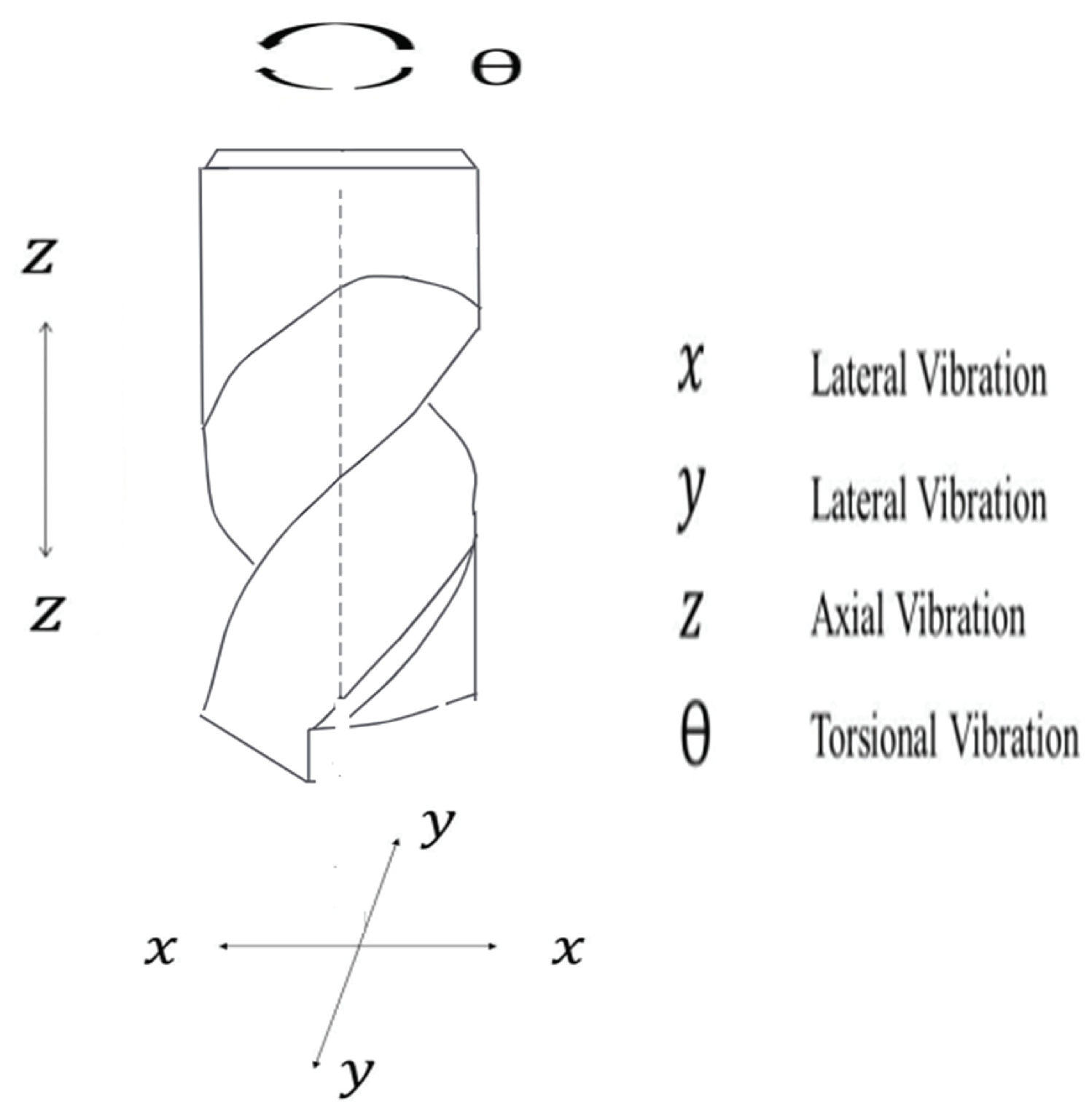
The vibration in the drilling tool system can be resolved along three components (4 DOF), which is shown in Figure 1.
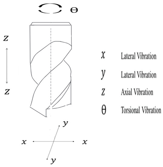
Figure 1.
Three modes of vibration (4 DOF) in drilling tools.
The lateral vibrations along two components (), axial vibration (z) as well as torsional vibration () associated with the drilling tool are modeled as [48,49]:
here, the vibration is represented by X, and the cutting force is illustrated by , stated as:
In addition,
In addition, and . Again, mass = , damping matrix = , stiffness matrix = and spindle speed dependent = Again, (, ), (, ) and (, ) are the modal masses, stiffness and damping constants of the most flexible mode along two main components (x,y) of the drill bit, respectively. The vector associated with the cutting force can be represented as follows:
In addition,
The diagonal coefficient matrices are and [50]. The nonlinear nature of the cutting forces is an important factor and has to be handled in an appropriate manner. The governing equation associated with the drilling process can be achieved as follows using Equations (1) and (4):
Here, time delay is signified by T. A controller is used to generate the control forces required to control the drilling operation. Discretizing Equation (6) with a control force is:
and the control is illustrated as . The state space form of Equation (7) is illustrated as:
where
where z represents vibration state vector associated with vibration at time interval t. In addition, and are constants. The identity matrices are 0 and I, respectively. represents the constant input matrix to define the controller. Now the continuous-time model is transformed into discrete-model by keeping both the control force and cutting forces constant during the sampling period ,
Now, the state vector is illustrated as , the state matrix is , and the input vector is . In addition, is the scalar input. The associated nonlinearity is embedded in the cutting forces represented by v(. In addition, represents the matrix to define the cutting force.
Type-2 Takagi–Sugeno(IT2 T–S) Fuzzy System
Fuzzy Technique description: For example, if , are type-2 fuzzy sets, then the type-2 fuzzy set A with the membership function is defined as
where is an auxiliary variable, is the primary membership function. For the type-2 fuzzy set A,
The integral ∫ of the classical fuzzy set becomes the sum ∑.
The upper and lower membership functions are defined as and They describe the upper and lower bounds of the uncertainties. For i-th rule and the point the crisp input is fuzzified in the interval of
where ∗ denotes the t-norm operator, it can be the minimization.
For all l rules, type-2 fuzzy inference engine aggregates with the fuzzified inputs and infers another type-2 fuzzy set,
where represents the membership function of the fired rule, which is expressed by extended sup-star composition. For details on it, please refer to [51].
We use the type-reduction method to convert into a type-1 fuzzy set. This technique captures more information about rule uncertainties than does the defuzzified value (a crisp number), and seems to be as fundamental to the design of fuzzy logic systems that include linguistic uncertainties (that translate into rule uncertainties) as variance is to the mean in case of probabilistic uncertainties. The centroids associated with type-2 fuzzy sets are calculated. For the i-th rule, the centroid of j-the output fuzzy rule is , and are the most left and right points. The type-2 fuzzy sets are reduced to the type-1 fuzzy set with the interval The most popular technique for type-reducing an interval type-2 fuzzy set is the Karnik–Mendel (KM) iterative procedure. The outcome of type-reduction of an interval type-2 fuzzy set is an interval type-1 set considering the criteria that the centroid is placed between the two endpoints. The iterative methodology is a superior technique in order to find these endpoints. The centroid of the type-1 set is considered to be the centre of this interval.
For all p rules,
where and are the firing strengths associated with and of i-th rule. By the minimization and maximization operation, and can be expressed as
where By singleton fuzzifier, the jth output of the fuzzy logic system can be expressed as
where is the point at which is the point at which .
The plant dynamics which is nonlinear in nature can be described by employing a p-rule IT2 T–S fuzzy model [36,38]. The rule is formulated in such a manner that the antecedent has IT2 fuzzy sets, whereas the consequent is represented by a linear dynamical system as follows:
Here, is termed as an IT2 fuzzy logic set having a rule which is j corresponding to the function , also ; is a positive integer. The illustration of the state vector associated with the system is represented by . Again, A and B are the unknown system and unknown input matrices, respectively. The input vector is illustrated as . The pattern of type-2 fuzzy set is [52]:
where and represents the numerical illustration of left and right most points, respectively, as:
also, ] and and termed as firing strengths of and of rule . The discrete-time nonlinear system represented by Equation (11) along with fault dynamics can be represented by an IT2 T–S fuzzy model with r rules as:
The Rule in Details:
If is AND……AND is THEN, the discretized state space system with output will be:
where stated as an interval type-2 fuzzy set having rule i associated with the function r = the number of IF-THEN rules. Again, with p considered to be positive integer. In addition, is the systems state vector, is the output, is the system input, and is the unknown bounded system uncertainty. The concept of firing strength having the rule is of the following interval sets:
where
in which and illustrates the lower grade of membership, upper grade of membership, lower membership function, and upper membership function, respectively. The IT2 T–S fuzzy model [1,53] can be illustrated as follows:
where and Relying on the stated Equation (20), the weighting functions associated with the type-2 fuzzy are:
In this stage, it is important to prove that the identification error is bounded; therefore, the fault dynamics are considered to be constant and therefore:
where is the positive definite matrix. Thus, using Equations (27) and (28) in Equation (26),
In addition, the weighting functions satisfy the convex sum property depicted as:
in which , , and are nonlinear functions, and are the concerned membership functions. In addition, Equation (27) states the type reduction.
In addition, and are the fuzzy weighting functions. For (27), the implementation of the learning laws takes place in the following manner:
and are stated by the equations mentioned below:
also and The dead-zone parameter is represented by and . Again, and are represented by:
The modeling error satisfies the equation below:
is the state of the fuzzy model, also from Equation (29):
where and are positive constants, and are design parameters.
In order to analyze the stability of the training algorithm (31), the dynamics of the modeling error are required. Thus, (35) can be expressed as:
where and are unknown optimal weights, , , , , and are approximation errors, such as
The error dynamics are from (35) and (37),
where and and are the remainders of the Taylor formula for and , respectively.
The next theorem provides proof of the stability of the fuzzy modeling. It is for the identification of the nonlinear system using Type 2 fuzzy thus validating that identification error is bounded.
Theorem1.
Proof.
The candidate for Lyapunov analysis is chosen as follows:
In addition, the following relation is valid , so:
Since the modeling error is bounded as
in order that
Therefore, it is proved that is bounded. In addition, if then, from (31), it is evident that the weights do not change and hence they are bounded. In addition, in this stage, it is assumed that the fault dynamics are not changing due to the non occurrence of faults. This theorem validates that the fuzzy modeling approach can be implemented with assured stability. The next stage is the fault detection scheme where an innovative observer will be developed to detect faults in the drilling bit with respect to the vibration measurements. □
3. The Technique of Fault Detection
A general fault dynamics equation is illustrated as [1]:
In the above equation, the unknown fault magnitude is depicted by . The fault dynamics time profile is represented by The intention of using time profile factor is for extracting general occurring fault dynamics associated with the nonlinear system. The fault basis function, which is a known quantity, is stated as . The time profile [54] is illustrated as:
The rate of growth of fault is given by . The relation depicting abrupt faults is given by:
where is the time of fault occurrence, For the purpose of monitoring the system represented by Equation (26), a fault detection observer is chosen as:
the representation of the system state is done in this manner , is the calculated output, and illustrates the observer gain. In addition,
represents the state residual and the output residual, respectively. Now, the error dynamics before the fault commencement are:
In addition, the state and output residuals after the detection of the fault:
where the parameter estimation error is signified by . In addition, = discrete time approximation (ADT). Using the concept of Z-transform applied by Zheng et al. [55], the FD residual can be expressed as:
where and are constant design matrix. The involved nonlinearity is represented by If the below mentioned conditions are satisfied, then it can be separated from the FD residual.
Condition 1
Condition 2
The conditions Equations (58) and (59) are utilized to extract the values of observer gains. Now, we propose that . In addition, and Using Equation (55):
The following updated laws will be used to verify that the state residual and parameter estimate error are uniformly bounded, which also confirms that the output residual is uniformly bounded:
Theorem2.
The boundary condition of the output residual and the parameter estimation error will be validated if the conditions stated below are satisfied:
when a discrete time observer is used to monitor a nonlinear system that has been updated with new laws. Equations (61) and (62) are utilized for the unknown parameter tuning process linked to ADT
Proof.
Consider Lyapunov candidate function as:
The first difference of the Equation (63) is given by:
Now, let
Re-arranging the terms in Equation (67) and
Now, considering
Arranging Equation (72) and applying Cauchy–Schwarz inequality criteria:
Now, the boundary conditions for the following terms can be set:
using Equation (74) and conditions (75), also
Now, if and only if
(1)
and (2)
which yields
It is now proved by the theorem that the system states are bounded, which is very important from a stability concern of the fault detector system. If during any point the system states are not stable, the fault detector will generate unstable results, thus decreasing the effectiveness of the entire process. It also validates that the fault detection estimator is reliable with precise online learning of the fault magnitude. □
4. Validation and Results
The drilling process parameters illustrated in [48] were implemented for drilling process simulation to verify the efficacy of the created theory and to confirm the notion of the new fault detection technique. The parameters are shown in Table 1:

Table 1.
Parameters.
Simulation of the Drilling Process for Verification
Equation (7) can be represented along and components as follows:
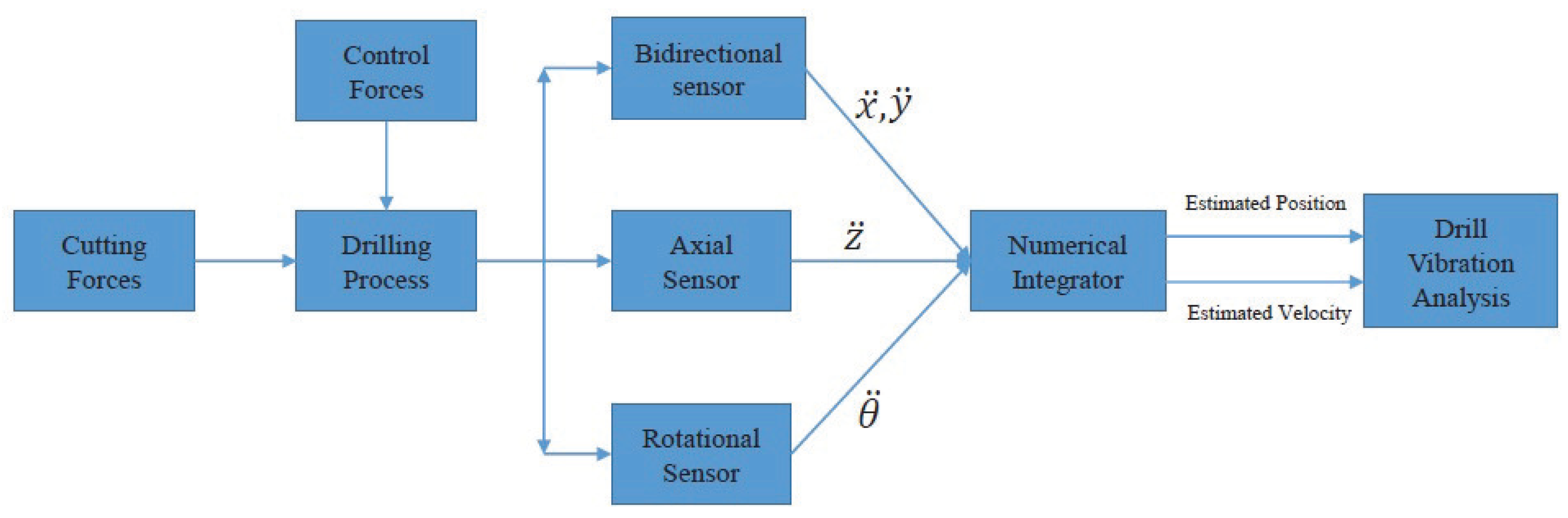
where and are the accelerations along and the component. In Figure 2 and Figure 3, the block diagrams depict the simulation of the drilling process without and with faults, respectively. By utilizing Equation (78), the acceleration signals along x, y, z, and directions are obtained. These accelerations are then fed to the numerical integrator for the generation of velocity and position signals. These signals are used for the vibration analysis of the drill bit. The vibration signals along x, y, z, and directions will vary in the events of the fault in the drill tool. For simplicity, the analysis results along x and y directions are demonstrated. The nonlinear cutting forces implemented for the simulation process along x and y directions are given by [56]:

Figure 2.
Block diagram of drilling simulation without fault.
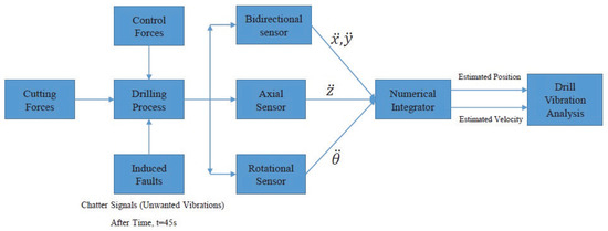
Figure 3.
Block diagram of drilling simulation with induced fault.
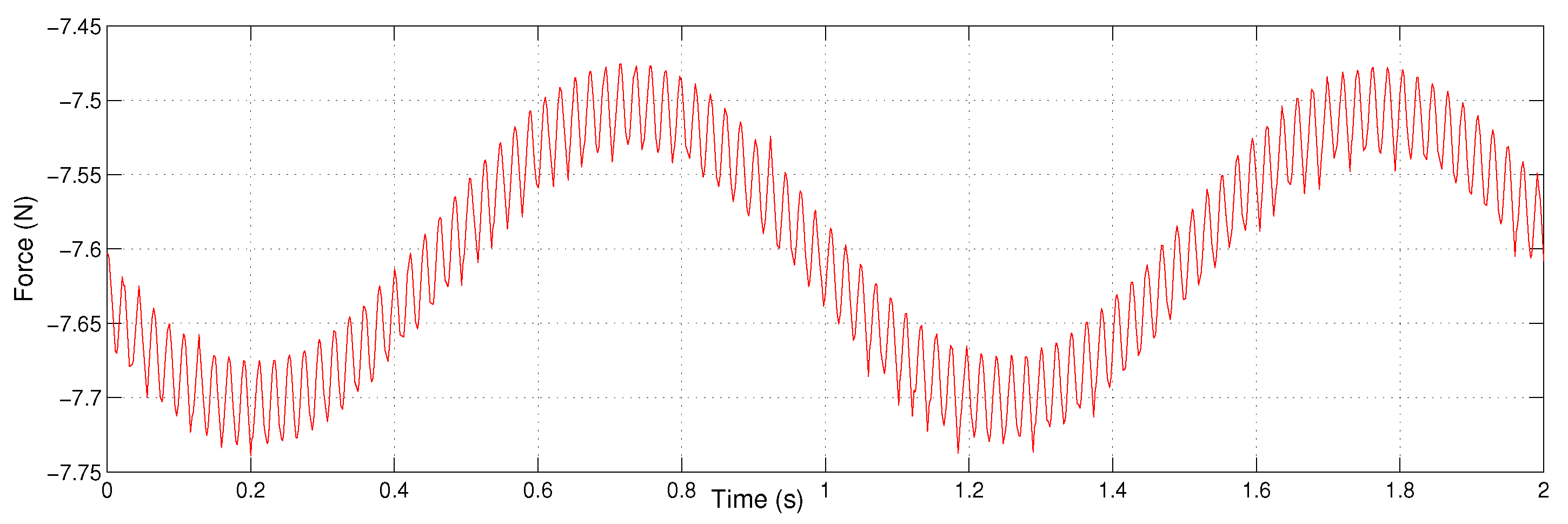
Equation (79) is utilized to generate the cutting forces for the drilling process. The cutting forces for a period of 2s along the components x and y and are represented using Figure 4 and Figure 5, respectively.
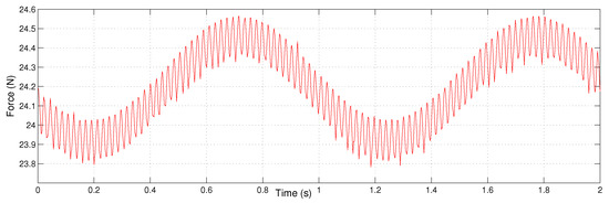
Figure 4.
x-axis representation of cutting force.
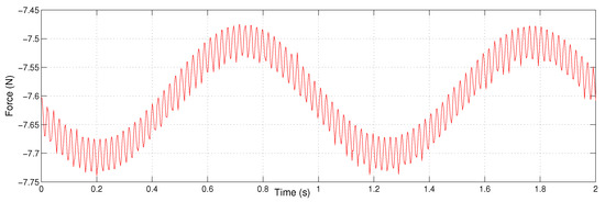
Figure 5.
y-axis representation of cutting force.
The accelerations in case of the real process can be calculated by installing accelerometer sensors on the drilling machine. Types of sensors which can be used for the process can be categorized as:
- (a)
- Bidirectional sensor—For the computation of x and y components of accelerations;
- (b)
- Axial sensor in order to calculate the acceleration along z direction;
- (c)
- Rotational sensor in order to calculate the acceleration along the direction.
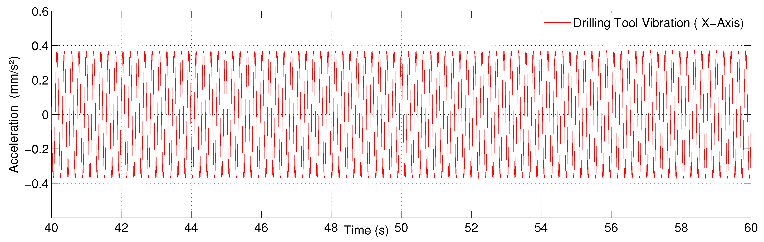
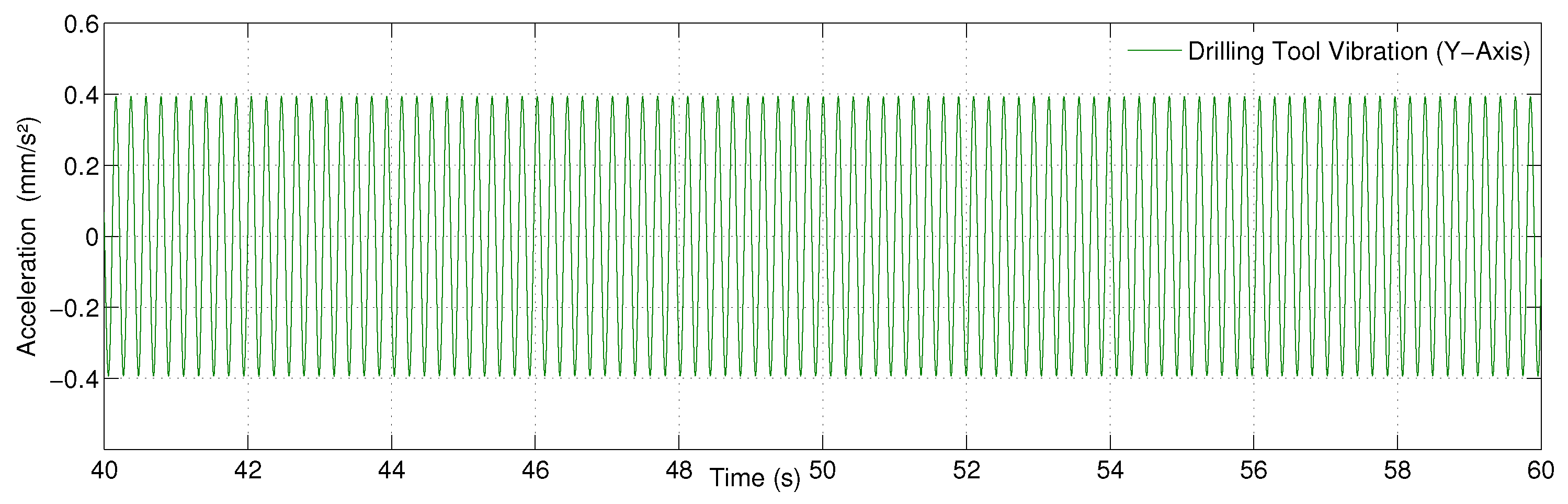
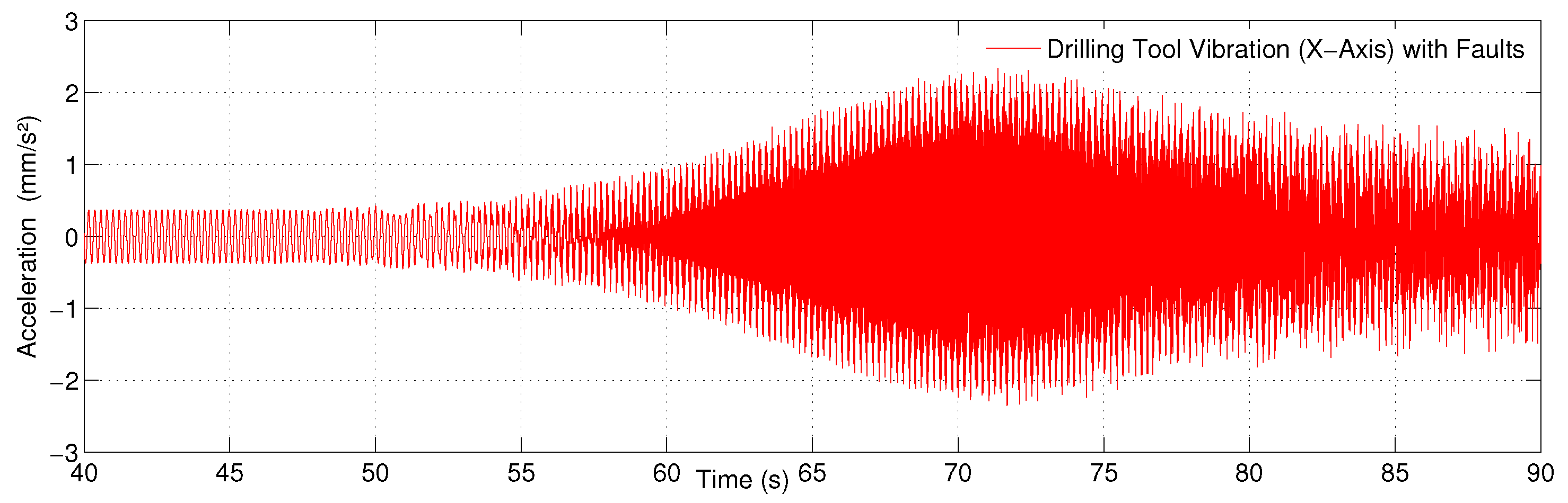
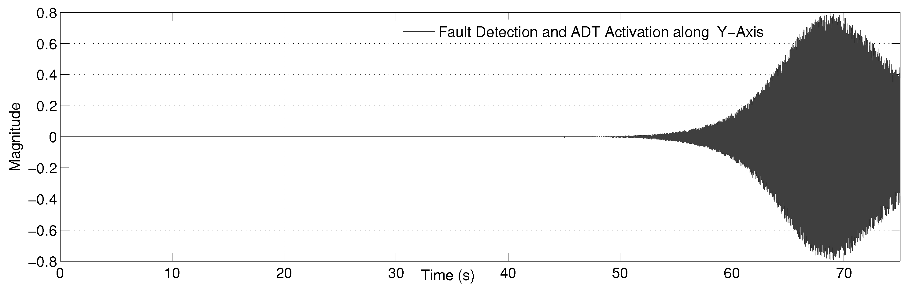
The entire drilling mechanism is simulated using the software platform Matlab/Simulink. The events of faults demonstrated using simulation are presented and consequently validated the fault detector scheme for successful detection of faults. For the drilling process model, two subsystem Simulink blocks are used. One block with the defect and the second block without the fault are used to compare the findings. Control signals and cutting forces are the process model’s inputs. The simulation time was set for a period of 120 s. The IT2-FLS toolbox designed by Taskin et al. [57] is implemented in order to actuate the simulation process. The important features of the IT2-FLS toolbox are the main editor, membership function editor, rule editor as well as the surface viewer. The membership functions considered for the entire process are the Gaussian functions. Designing the type-2 fuzzy system, we first use the type-2 fuzzy logic system toolkit [57]. The computing cost of calculating the type-2 fuzzy system output is high due to its iterative nature [58]. To deal with these conditions, many TR approaches for decreasing the computational cost of the type-2 fuzzy inference mechanism have been presented. In the fuzzy logic theory, the Karnik–Mendel (KM) algorithms are iterative techniques.They are known to converge monotonically and super exponentially quickly; however, convergence requires several (typically two to six) iterations [59]. The TR methods were divided into two categories by Wu: Enhancements to the KMs, which reduced the KM’s computational cost, and Alternative TR approaches, which are closed-form approximations to the KM algorithm [60]. Because of its novelty and adaptability, the KM approach is the most popular [61]. A type-2 fuzzy logic system toolbox supports type reduction and defuzzification procedures: (1) Karnik–Mendel Algorithm (KM); (2) Enhanced KM Algorithm (EKM); (3) Iterative Algorithm with Stop Condition (IASC); (4) Enhanced IASC (EIASC); (5) Enhanced Opposite Direction Searching Algorithm (EODS); (6)Wu–Mendel Uncertainty Bound Method (WM); (7) Nie–Tan Method (NT); and (8) Begian–Melek–Mendel Method (BMM). It is possible to state the antecedent MFs using the MF types that currently exist in the Matlab Fuzzy Logic Toolbox in the type-2 fuzzy logic system toolbox. As a result, the LMF and UMF Matlab functions can be implemented in the same style. However, each type of MF has an additional parameter that represents the height of the related MF. A triangle MF, for example, is defined by the parameters A2, B2, C2, and H2, which specify the MF’s left point, centre point, right point, and height, respectively. In type-2 fuzzy systems, especially type-2 fuzzy controller design, the parameter H2 is commonly used to produce FOU. Gaussian functions are used for the membership functions. Gaussian membership functions have the advantage of being easier to design since they are easier to express and optimise, they are always continuous, and they are faster for small rule bases. When the same number of MFs and the same type-reduction and defuzzification approach are utilised, Gaussian type-2 fuzzy logic systems are faster than trapezoidal type-2 fuzzy logic systems. Because small rule bases are commonly employed in practise, Gaussian type-2 fuzzy logic systems appear to be more cost-effective. The type-2 fuzzy system is defuzzified by implementing the technique proposed in [36]. The fuzzy laws are chosen on the basis of Theorem 1 concentrating on the condition The learning rate used for the fuzzy laws is The conditions extracted from Theorem 2 for the fault detector estimator are and . In Figure 6 and Figure 7, the drill tool’s vibration is plotted on the x and y axes. For better clarity of the plot representation, a 20-s interval is shown. These vibration graphs show the pattern of vibration in the absence of induced flaws. At 45 s following the commencement of the drilling process, an artificial fault is induced along the x and y axes to the drilling operation simulation. The vibration of the drill tool with the induced flaws is represented by Figure 8 and Figure 9. These plots show how plots with chatter change after 45 s, proving the fluctuation of vibration caused by induced faults. The period between 40 s and 90 s is illustrated for the clarity of the charts.The induced fault is a self generated sinusoidal signal. The defect detection in the drill tool is shown in Figure 10 and Figure 11 along x and y components. The charts show that there is no change in the signal until 45 s, when it displays zero. At the instant of the detection of fault, the change in vibration signal is detected instantly along x and y components. From the vibration plots with induced faults (Figure 8 and Figure 9), it is clear that the intensity of the faults increases after a period of 65 s. However, from the fault detection estimator, the variation of the plots is noticed instantly with the fault starting up, thus raising an alarm and preventing the damage of drill tool. Hence, it is validated that the interval type-2 (IT2) Takagi–Sugeno (T–S) fuzzy based observer fault detection algorithm is successful as a fault detector mechanism by the sounding alarm after a period of 45 s. The future work is intended towards the investigation of faults along z and directions and comparing the results with x and y directions, thus predicting remaining useful life (RUL) of the drilling process system.
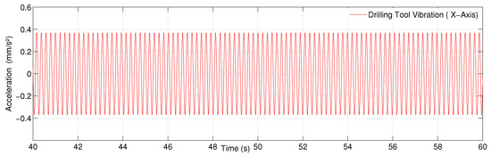
Figure 6.
Drilling Tool vibration along the x-direction.
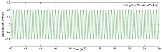
Figure 7.
Drill Tool vibration along the y-direction.

Figure 8.
Drilling Tool vibration along the x-direction with the induced fault.
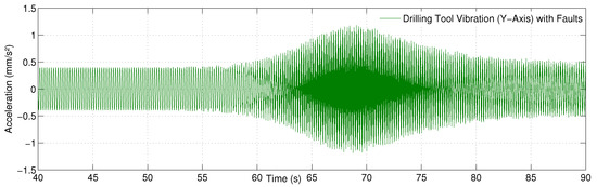
Figure 9.
Drilling Tool vibration along the y-direction with induced fault.
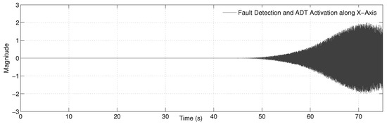
Figure 10.
Fault detection scheme along the x-axis.

Figure 11.
Fault detection scheme along the y-axis.
5. Conclusions
This work shows how to find faults in the drilling process using an interval type-2 (IT2) Takagi–Sugeno (T–S) fuzzy-based observer fault detection system. In the face of system uncertainty, the stability of the system using the fault detection estimator is validated. This system uncertainty is tackled using the type-2 fuzzy logic system. Theorem 1 is developed to validate the stability of Type-2 fuzzy modeling. The system states of the process are proved to be bounded, which also validates the stability of the fault detection estimator using Theorem 2. The stability requirements of Theorem 1 and Theorem 2 are fulfilled using the Lyapunov stability candidate. The defect detection system’s effectiveness is verified using numerical analysis, which also establishes theoretical features. The main intention of this paper is to develop a control-based fault algorithm to detect an induced fault at the correct instant with assured stability of the system. This type of unique way for detecting a flaw in a drilling system has never been used before. The effective methodology can be implemented in real-time for detecting faults during drilling operations. This is critical for increasing the productivity and quality of the machining process, and it also helps improve the surface finish of the work piece satisfying the customer needs and expectations. Future work is intended towards the computation of Remaining Useful Life (RUL) of the drilling devices.
Author Contributions
Conceptualization, S.P., R.T. and D.K.; Methodology, S.P., R.T. and D.K.; Software, S.P.; Validation, M.L. and S.P.; Investigation, S.P., R.T. and D.K.; Writing—original draft preparation, S.P., R.T. and D.K.; Writing—review and editing, S.P.; Supervision, M.L.; Project administration, M.L.; Funding acquisition, M.L. All authors have read and agreed to the published version of the manuscript.
Funding
This research received no external funding.
Institutional Review Board Statement
Not applicable.
Informed Consent Statement
Not Applicable.
Data Availability Statement
Study did not report any data.
Acknowledgments
Magnus Löfstrand gratefully acknowledges VINNOVA research funding in the project A digital twin to support sustainable and available production as a service and Swedish Mining Innovation funding in the project. A general digital twin driving mining innovation through statistical and logical modelling.
Conflicts of Interest
The authors declare no conflict of interest.
References
- Thumati, B.T.; Feinstein, M.A.; Jagannathan, S. A Model-Based Fault Detection and Prognostics Scheme for Takagi–Sugeno Fuzzy Systems. IEEE Trans. Fuzzy Syst. 2014, 22, 736–748. [Google Scholar] [CrossRef]
- Patton, R.J.; Frank, P.M.; Clark, R.N. Issues of Fault Diagnosis for Dynamic Systems; Springer: London, UK, 2000. [Google Scholar]
- Blanke, M.; Kinnaert, M.; Lunze, J.; Staroswiecki, M. Diagnosis and Fault-Tolerant Control, 2nd ed.; Springer: Berlin/Heidelberg, Germany, 2006. [Google Scholar]
- Youssef, T.; Chadli, M.; Karimi, H.R.; Wang, R. Actuator and sensor faults estimation based on proportional integral observer for TS fuzzy model. J. Frankl. Inst. 2017, 354, 2524–2542. [Google Scholar] [CrossRef]
- Benbouzid, M.E.H.; Vieira, M.; Theys, C. Induction motors’ faults detection and localization using stator current advanced signal processing techniques. IEEE Trans. Power Electron. 1999, 14, 14–22. [Google Scholar] [CrossRef]
- Widodo, A.; Yang, B.S.; Gu, D.S.; Choi, B.K. Intelligent fault diagnosis system of induction motor based on transient current signal. Mechatronics 2009, 19, 680–689. [Google Scholar] [CrossRef]
- Isermann, R. Model-based fault-detection and diagnosis—Status and applications. Annu. Rev. Control 2005, 29, 71–85. [Google Scholar] [CrossRef]
- Zarei, J.; Tajeddini, M.A.; Karimi, H.R. Vibration analysis for bearing fault detection and classification using an intelligent filter. Mechatronics 2014, 24, 151–157. [Google Scholar] [CrossRef]
- Gertler, J. Survey of model-based failure detection and isolation in complex plants. IEEE Control Syst. Mag. 1988, 8, 3–11. [Google Scholar] [CrossRef]
- Frank, P. Fault diagnosis in dynamic systems using analytical and knowledge-based redundancy—A survey and some new results. Automatica 1990, 26, 459–474. [Google Scholar] [CrossRef]
- Garcia, E.; Frank, P. Deterministic nonlinear observer-based approaches to fault diagnosis: A survey. Control Eng. Pract. 1997, 5, 663–670. [Google Scholar] [CrossRef]
- Gao, Z.; Cecati, C.; Ding, S.X. A Survey of Fault Diagnosis and Fault-Tolerant Techniques—Part I: Fault Diagnosis With Model-Based and Signal-Based Approaches. IEEE Trans. Ind. Electron. 2015, 62, 3757–3767. [Google Scholar] [CrossRef]
- Kuestenmacher, A.; Plöger, P.G. Model-Based Fault Diagnosis Techniques for Mobile Robots**This work was sponsored by the B-IT foundation and the Strukturfond des Landes Nordrhein-Westfalen for the female PhD students. IFAC-PapersOnLine 2016, 49, 50–56. [Google Scholar] [CrossRef]
- Kommuri, S.K.; Defoort, M.; Karimi, H.R.; Veluvolu, K.C. A Robust Observer-Based Sensor Fault-Tolerant Control for PMSM in Electric Vehicles. IEEE Trans. Ind. Electron. 2016, 63, 7671–7681. [Google Scholar] [CrossRef]
- Li, L.; Ding, S.X.; Qiu, J.; Yang, Y.; Xu, D. Fuzzy Observer-Based Fault Detection Design Approach for Nonlinear Processes. IEEE Trans. Syst. Man Cybern. Syst. 2017, 47, 1941–1952. [Google Scholar] [CrossRef]
- Teti, R.; Jemielniak, K.; O’Donnell, G.; Dornfeld, D. Advanced monitoring of machining operations. CIRP Ann. Manuf. Technol. 2010, 59, 717–739. [Google Scholar] [CrossRef]
- Canizo, M.; Onieva, E.; Conde, A.; Charramendieta, S.; Trujillo, S. Real-time predictive maintenance for wind turbines using Big Data frameworks. In Proceedings of the 2017 IEEE International Conference on Prognostics and Health Management (ICPHM), Dallas, TX, USA, 19–21 June 2017; pp. 70–77. [Google Scholar]
- Quintana, G.; Ciurana, J. Chatter in machining processes: A review. Int. J. Mach. Tools Manuf. 2011, 51, 363–376. [Google Scholar] [CrossRef]
- Bustillo, A.; Correa, M.; Reñones, A. A Virtual Sensor for Online Fault Detection of Multitooth-Tools. Sensors 2011, 11, 2773–2795. [Google Scholar] [CrossRef] [PubMed]
- Kumar, A.; Ramkumar, J.; Verma, N.K.; Dixit, S. Detection and classification for faults in drilling process using vibration analysis. In Proceedings of the 2014 International Conference on Prognostics and Health Management, Cheney, WA, USA, 22–25 June 2014; pp. 1–6. [Google Scholar]
- Goyal, D.; Pabla, B.S. Condition based maintenance of machine tools—A review. CIRP J. Manuf. Sci. Technol. 2015, 10, 24–35. [Google Scholar] [CrossRef]
- Roth, J.T.; Djurdjanovic, D.; Yang, X.; Mears, L.; Kurfess, T. Quality and Inspection of Machining Operations: Tool Condition Monitoring. ASME J. Manuf. Sci. Eng. 2010, 132, 041015. [Google Scholar] [CrossRef]
- Pimenov, D.Y.; Bustillo, A.; Mikolajczyk, T. Artificial intelligence for automatic prediction of required surface roughness by monitoring wear on face mill teeth. J. Intell. Manuf. 2018, 29, 1045–1061. [Google Scholar] [CrossRef]
- Kuntoğlu, M.; Aslan, A.; Pimenov, D.Y.; Usca, Ü.A.; Salur, E.; Gupta, M.K.; Mikolajczyk, T.; Giasin, K.; Kapłonek, W.; Sharma, S. A Review of Indirect Tool Condition Monitoring Systems and Decision-Making Methods in Turning: Critical Analysis and Trends. Sensors 2021, 21, 108. [Google Scholar] [CrossRef] [PubMed]
- Fan, S.-K.S.; Hsu, C.-Y.; Tsai, D.-M.; He, F.; Cheng, C.-C. Data-Driven Approach for Fault Detection and Diagnostic in Semiconductor Manufacturing. IEEE Trans. Autom. Sci. Eng. 2020, 17, 1925–1936. [Google Scholar] [CrossRef]
- Luo, B.; Wang, H.; Liu, H.; Li, B.; Peng, F. Early Fault Detection of Machine Tools Based on Deep Learning and Dynamic Identification. IEEE Trans. Ind. Electron. 2019, 66, 509–518. [Google Scholar] [CrossRef]
- Zadeh, L.A. Fuzzy sets as a basis for a theory of possibility. Fuzzy Sets Syst. 1978, 1, 3–28. [Google Scholar] [CrossRef]
- Zadeh, L.A. Fuzzy Sets. Inf. Control 1965, 8, 338–353. [Google Scholar] [CrossRef]
- Zadeh, L.A. From computing with numbers to computing with words—From manipulation of measure-ments to manipulation of perceptions. IEEE Trans. Circuits Syst. I Fundam. Theory Appl. 1999, 45, 105–119. [Google Scholar] [CrossRef]
- John, R.; Coupl, S. Type-2 fuzzy logic: A historical view. IEEE Comput. Intell. Mag. 2007, 2, 57–62. [Google Scholar] [CrossRef]
- Mendel, J.M. Type-2 Fuzzy Sets as Well as Computing with Words. IEEE Comput. Intell. Mag. 2019, 14, 82–95. [Google Scholar] [CrossRef]
- Takagi, T.; Sugeno, M. Fuzzy identification of systems and its applications to modeling and control. IEEE Trans. Syst. Man Cybern. 1985, 15, 116–132. [Google Scholar] [CrossRef]
- Nguang, S.K.; Shi, P.; Ding, S. Fault detection for uncertain fuzzy systems: An LMI approach. IEEE Trans. Fuzzy Syst. 2007, 15, 1251–1262. [Google Scholar] [CrossRef]
- Barnes, M.R. Neuro-Fuzzy Clustering of Radiographictibia Image Data Using Type-2 Fuzzy Sets. Inf. Sci. 2000, 125, 65–82. [Google Scholar]
- Mendel, J.M. Uncertain Rule-Based Fuzzy Logic Systems: Introduction and New Directions; Prentice Hall PTR: Upper Saddle River, NJ, USA, 2001. [Google Scholar]
- Liang, Q.; Mendel, J.M. Interval Type-2 Fuzzy Logic Systems: Theory and Design. IEEE Trans. Fuzzy Syst. 2002, 8, 535–550. [Google Scholar] [CrossRef]
- Sepúlveda, R.; Castillo, O.; Melin, P.; Rodríguez-Díaz, A.; Montiel, O. Experimental Study of Intelligent Controllers Under Uncertainty using Type-1 and Type-2 Fuzzy Logic. Inf. Sci. 2007, 177, 2023–2048. [Google Scholar] [CrossRef]
- Lam, H.K.; Li, H.; Deters, C.; Wuerdemann, H.A.; Secco, E.; Althoefer, K. Control design for interval type-2 fuzzy systems under imperfect premise matching. IEEE Trans. Ind. Electron. 2014, 61, 956–968. [Google Scholar] [CrossRef]
- Román-Flores, H.; Chalco-Cano, Y.; Figueroa-García, J.C. A note on defuzzification of type-2 fuzzy intervals. Fuzzy Sets Syst. 2020, 399, 133–145. [Google Scholar] [CrossRef]
- Biglarbegian, M.; Mendel, J.M. On the Justification to Use a Novel Simplified Interval Type-2 Fuzzy Logic System. J. Intell. Fuzzy Syst. 2015, 28, 1071–1079. [Google Scholar] [CrossRef]
- Castillo, O.; Melin, P. A review on interval type-2 fuzzy logic applications in intelligent control. Inf. Sci. 2014, 279, 615–631. [Google Scholar] [CrossRef]
- Paul, S.; Morales-Menendez, R. Active Control of Chatter in Milling Process Using Intelligent PD/PID Control. IEEE Access 2018, 6, 72698–72713. [Google Scholar] [CrossRef]
- Paul, S.; Lofstrand, M. Intelligent Fault Detection Scheme for Drilling Process. In Proceedings of the 2019 7th International Conference on Control, Mechatronics and Automation (ICCMA), Delft, The Netherlands, 6–8 November 2019; pp. 347–351. [Google Scholar]
- Li, H.; Gao, Y.; Shi, P.; Lam, H. Observer-Based Fault Detection for Nonlinear Systems With Sensor Fault and Limited Communication Capacity. IEEE Trans. Autom. Control 2016, 61, 2745–2751. [Google Scholar] [CrossRef]
- Montazeri-Gh, M.; Yazdani, S. Application of interval type-2 fuzzy logic systems to gas turbine fault diagnosis. Appl. Soft Comput. 2020, 96, 106703. [Google Scholar] [CrossRef]
- Maged, A.; Xie, M. Uncertainty utilization in fault detection using Bayesian deep learning. J. Manuf. Syst. 2022, 64, 316–329. [Google Scholar] [CrossRef]
- Jalayer, M.; Orsenigo, C.; Vercellis, C. Fault detection and diagnosis for rotating machinery: A model based on convolutional LSTM, Fast Fourier and continuous wavelet transforms. Comput. Ind. 2021, 125, 103378. [Google Scholar] [CrossRef]
- Ahmadi, K.; Altintas, Y. Stability of lateral, torsional and axial vibrations in drilling. Int. J. Mach. Tools Manuf. 2013, 68, 63–74. [Google Scholar] [CrossRef]
- Eynian, M.; Altintas, Y. Chatter stability of general turning operations with process damping. J. Manuf. Sci. Eng. 2009, 131, 1005–1010. [Google Scholar] [CrossRef]
- Altintas, Y. Manufacturing Automation: Metal Cutting Mechanics, Machine Tool Vibrations, and CNC Design; Cambridge University Press: New York, NY, USA, 2011. [Google Scholar]
- Karnik, N.-N.; Mendel, J.-M. An Introduction to Type-2 Fuzzy Logic Systems; USC Report; 1998; Available online: http://sipi.usc.edu/~mendel/report (accessed on 14 October 2021).
- Lin, T.C.; Liu, H.L.; Kuo, M.J. Direct Adaptive Interval Type-2 Fuzzy Control of Multivariable Nonlinear Systems. Eng. Appl. Artif. Intell. 2009, 22, 420–430. [Google Scholar] [CrossRef]
- Lam, H.K.; Seneviratne, L.D. Stability analysis of interval type-2 fuzzy-model-based control systems. IEEE Trans. Syst. Man Cybern. B Cybern. 2008, 38, 617–628. [Google Scholar] [CrossRef]
- Thumati, B.T.; Jagannathan, S. A Model-Based Fault-Detection and Prediction Scheme for Nonlinear Multivariable Discrete-Time Systems With Asymptotic Stability Guarantees. IEEE Trans. Neural Netw. 2010, 21, 404–423. [Google Scholar] [CrossRef]
- Zheng, Y.; Fang, H.; Wang, H.O. Takagi-sugeno fuzzy-model-based fault detection for networked control systems with Markov delays. IEEE Trans. Syst. Man Cybern. Part B Cybern. 2006, 36, 924–929. [Google Scholar] [CrossRef]
- Moradi, H.; Bakhtiari-Nejad, F.; Movahhedy, M.R.; Vossoughi, G. Stability improvement and regenerative chatter suppression in nonlinear milling process via tunable vibration absorber. J. Sound Vibrat. 2012, 331, 4668–4690. [Google Scholar] [CrossRef]
- Taskin, A.; Kumbasar, T. An Open Source Matlab/Simulink Toolbox for Interval Type-2 Fuzzy Logic Systems. In Proceedings of the 2015 IEEE Symposium Series on Computational Intelligence, Cape Town, South Africa, 7–10 December 2015. [Google Scholar]
- Wu, D.; Nie, M. Comparison and practical implementation of type reduction algorithms for type-2 fuzzy sets and systems. In Proceedings of the 2011 IEEE International Conference on Fuzzy Systems (FUZZ-IEEE 2011), Taipei, Taiwan, 27–30 June 2011. [Google Scholar]
- Wu, D.; Mendel, J.M. Enhanced Karnik-Mendel algorithms. IEEE Trans. Fuzzy Syst. 2009, 17, 923–934. [Google Scholar]
- Wu, D. Approaches for reducing the computational cost of interval type-2 fuzzy logic systems: Overview and comparisons. IEEE Trans. Fuzzy Syst. 2013, 21, 80–99. [Google Scholar]
- Wu, D. On the Fundamental Differences between Type-1 and Interval Type-2 Fuzzy Logic Controllers. IEEE Trans. Fuzzy Syst. 2012, 10, 832–848. [Google Scholar] [CrossRef]


Publisher’s Note: MDPI stays neutral with regard to jurisdictional claims in published maps and institutional affiliations. |
© 2022 by the authors. Licensee MDPI, Basel, Switzerland. This article is an open access article distributed under the terms and conditions of the Creative Commons Attribution (CC BY) license (https://creativecommons.org/licenses/by/4.0/).