Article

Eyes versus Eyebrows: A Comprehensive Evaluation Using the Multiscale Analysis and Curvature-Based Combination Methods in Partial Face Recognition

Department of Electrical Engineering, Universitas Indonesia, Kampus Baru UI Depok, Depok City 16424, Indonesia
*
Author to whom correspondence should be addressed.
Algorithms 2022, 15(6), 208; https://doi.org/10.3390/a15060208
Submission received: 24 May 2022 / Revised: 6 June 2022 / Accepted: 11 June 2022 / Published: 14 June 2022
(This article belongs to the Special Issue Mathematical Models and Their Applications III)

Abstract

:
This work aimed to find the most discriminative facial regions between the eyes and eyebrows for periocular biometric features in a partial face recognition system. We propose multiscale analysis methods combined with curvature-based methods. The goal of this combination was to capture the details of these features at finer scales and offer them in-depth characteristics using curvature. The eye and eyebrow images cropped from four face 2D image datasets were evaluated. The recognition performance was calculated using the nearest neighbor and support vector machine classifiers. Our proposed method successfully produced richer details in finer scales, yielding high recognition performance. The highest accuracy results were 76.04% and 98.61% for the limited dataset and 96.88% and 93.22% for the larger dataset for the eye and eyebrow images, respectively. Moreover, we compared the results between our proposed methods and other works, and we achieved similar high accuracy results using only eye and eyebrow images.

1. Introduction

A face recognition system is a methodological technique that aims to find the correct matches between human face images and face datasets. Various applications utilize this system, such as identity verification, security and crime prevention, intelligent devices, robotic and computer interaction, and entertainment purposes in social media [1,2]. Face biometrics may better recognize individuals in a noninvasive way than other biometrics, such as through the iris, palm, vein, or fingerprint [3]. However, when the face is obstructed, the recognition system still has not achieved satisfactory performance. Obstruction of the face, known as face occlusion, occurs when objects hide part of the face [4].
There has been significant attention directed to masked face recognition research over the last three years due to the COVID-19 pandemic [5,6,7,8,9,10,11]. People must use a face mask in public places to prevent disease transmission. Using a face mask is one of the challenges in the face occlusion research topic. Partial face recognition using only the upper part of the face has become popular due to the occlusion-free condition in this area. The upper part of the face includes the forehead, eyes, and temporal region [12]. In addition, periocular biometrics (i.e., the rich information features around the eye) have been studied extensively in the last few years [13]. The periocular region is considered a substitute or additional feature due to its highly distinctive character and rich information [14].
Previous works focused on finding the best facial features for face recognition. Karczmarek et al. [15] used the analytic hierarchy process to estimate how important facial features were in face recognition. From one of the experiment results, the most discriminative features were the eyes, nose, and mouth. Conversely, although they noted that eyebrows were equally crucial in computational face recognition, they might not be essential in real-life situations. Peterson and Eckstein [16] studied the gaze behavior from human eye movement and its connection to identifying individuals. Their findings suggest that the saccades, rapid eye movements between fixation points, were located just below the eyes. Tome et al. [17] studied the effect of separating 15 face regions and found that the inner regions (mouth, nose, and right eyebrow) were more useful for images with a shorter acquisition distance, while the outer regions (forehead, chin, and right ear) were more suitable for a farther acquisition distance. Abudarham et al. [18] observed the critical features for face identification by intentionally changing features and tested the results of the perceptual effect. They found that several critical features vary slightly across variations of the equal identity and are robust to invariance problems. Continuing their work in [19], they discussed three critical findings: the eyebrow thickness, eye color and shape, and lip thickness were vital to identification. The same features could be used for familiar and unfamiliar faces, and the features essential in human evaluation were equally prominent for machine evaluation. Ding et al. [20] achieved detailed and precise detection of the major facial features by differentiating between features and the context of the features using subclass discriminant analysis (SDA) and subAdaBoost. Biswas et al. [21] proposed a one-shot frequency-dominant neighborhood structure to tackle problems when the area of the eyes is occluded. Wang et al. [22] proposed a combination of the vital subregions (eye, nose, and mouth) and the entire image to improve recognition performance.
The importance of facial features also helps to determine human race categorization and facial expression recognition. Bülthoff et al. [23] showed that the eyes are one factor in determining perceived biogeographic ancestry. From their investigation, Fu et al. [24] supported that the eyes, eyebrows, mouth, chin, and nose can be discriminative facial features for distinguishing the human race. Oztel et al. [25] utilized the eye and eyebrow regions using partial features for facial expression recognition. They achieved similar results compared to using full-face information. García-Ramírez et al. [26] also investigated the eyebrow and mouth areas for facial expression recognition.
As early as 2003, Sadr et al. [27] evaluated the importance of eyebrows in face recognition. Their findings recommend that the eyebrows are a significant feature in face recognition. The three possible reasons are as follows. First, the eyebrows carry emotions and other nonverbal signals. Second, the eyebrows may assist as a solid feature due to high contrast. They are robust against image degradation and illumination changes. Third, the eyebrows are considered a consistent feature because of the incredible variety among individuals and reliability across short periods of time (weeks or months). Various works analyzed eyebrow images for recognition. In their work, Yujian and Cihua [28] extracted string features. Hidden Markov models were employed in [29]. Turkoglu and Arican in [30] proposed the novel features of a three-patch local binary pattern and Weber local descriptor. Li et al. [31] designed fast template matching and a Fourier spectrum distance for an automatic human eyebrow recognition system. These previous works have shown that eyebrows have the potential to be future biometric traits.
Although they were highly distinctive, few works have investigated the value of adding a curvature-based method for the eyes and eyebrows to produce in-depth characteristics. In [32], curvature was added and combined with a gray level co-occurrence matrix (GLCM) and tested against a masked face recognition system. Although the added curvature did not improve the recognition’s performance, it successfully simplified the number of properties in the GLCM and the recognition’s running time. In [33], the periocular images were observed against the wavelet best basis (WBB) method. They were analyzed using wavelet characteristics and variations in geometry transformations and noisy images. Although the WBB improved the accuracy performance by 5–12%, the highest accuracy (86.33%) had not achieved satisfactory results.
In this work, we focused our observation on using the eye and eyebrow regions from face images datasets (cropped extended Yale B dataset [34,35], Aberdeen dataset [36], pain expression subset dataset [36], and real fabric face mask dataset [32]) to determine which feature was the most discriminative for a partial face recognition system. The eyes and eyebrows on the face have shapes that have details such as corners, lines, edges, and colors. Moreover, the eyebrows are located next to the forehead, therefore increasing their visibility [37]. A curvature-based method offers character to these details due to its ability to measure how curved a surface is. Generally, curvature-based methods need 3D images (where the third dimension offers the height value of the image data) [38,39,40], but in this research, we propose using 2D images and transforming them into three-dimensional data, where the third dimension contains the intensity value of the image. In addition, these periocular features may not offer distinctive details on the coarse scales but may be revealed on the finer scales. These finer scales can be obtained with the multiscale analysis method. Thus, we proposed an idea: combining the multiscale analysis methods (i.e., scale space (SS) and discrete wavelet transform (DWT)) with a curvature-based method.
This list contains the highlights and contributions of this work:
  • We compare the eyes and eyebrows to find the most discriminative facial feature for a partial face recognition system.
  • We evaluate the eye and eyebrow features with a combination of multiscale analysis and curvature-based methods. This combination aimed to capture the details of these features at finer scales and offer them in-depth characteristics using curvature. The combination using a curvature-based method was proven to improve the performance of the recognition system.
  • We demonstrate a comprehensive evaluation of all variables that occur due to combining multiscale analysis and curvature-based methods.
  • The results from the proposed methods are compared using the limited number of images versus the whole dataset. We also compare the results to other works with the condition of the same datasets, and we successfully achieve similar high-accuracy results using only eye and eyebrow images.

2. Materials and Methods
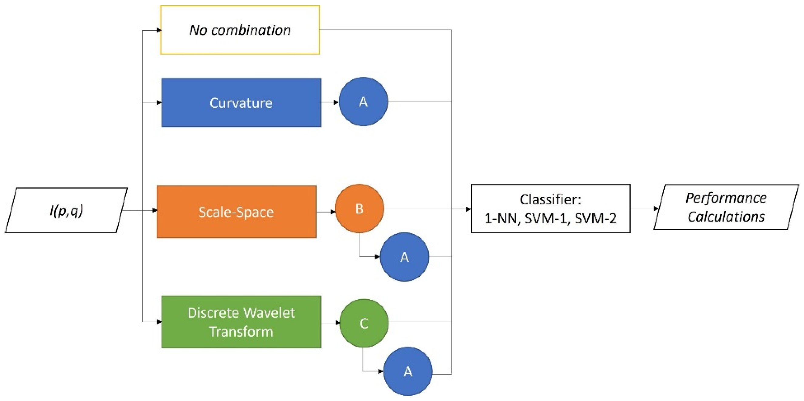
2.1. Methods

The overall flowchart appears in Figure 1. First, we addressed the original images (no combination) and the extracted curvature features (connector A) in the classifiers. The recognition system employed the scale-space method (connector B) and discrete wavelet transform (connector C). The scale-space method (SS) was built for four octaves and three levels in each octave. We created two decomposition levels with Haar, Symlet, Daubechies, and biorthogonal wavelets for the discrete wavelet transform (DWT). These four initial results were the foundation for evaluating whether our proposed methods successfully achieved better performance.
The following observation was to combine the scale space (SS) and discrete wavelet transform (DWT) with a curvature-based method (connector B + A and connector C + A). We evaluated the curvature-based methods with four curvatures: Gaussian, mean, max, and min principal curvatures. All observations were tested against four face image datasets and two classifiers (i.e., k-nearest neighbor (k-NN) and support vector machine (SVM)).

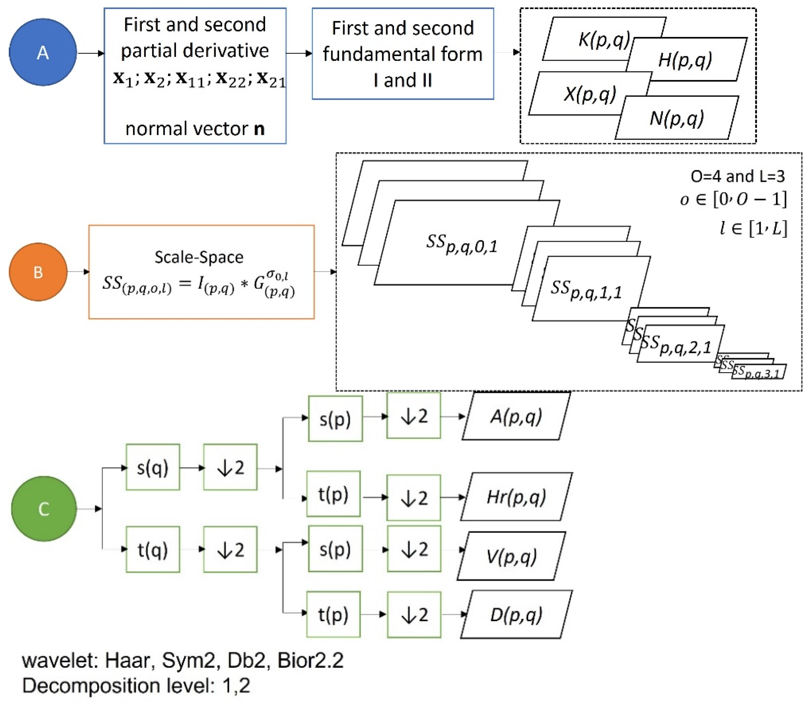
2.1.1. The Curvature-Based Method

To measure how a surface bends in 3 is to observe changes from each point on the surface. A grayscale image I(p,q) has p rows and q columns, and each combination of rows and columns contains a grayscale value of 0–255. Then, the two-dimensional data 2 is transformed into the three-dimensional data 3 . Row p and column q are transformed into the x-plane and y-plane, while the intensity value is transformed into the z-plane. Then, the curvature in this research is calculated from 3 of I(p,q) (Equation (1)), where the third dimension is not the height of the data but the intensity value of the images I:
I ( p , q ) I ( x , y , z )
I ( x , y , z ) has a surface in space where each point on the surface is parameterized using two coordinates [41]:
x : 2 U 3 : ( u , v ) x ( u , v )
The first partial derivative with respect to u and v is
x 1 = [ x u y u z u ] ;   x 2 = [ x v y v z v ]
From the first partial derivative, we can calculate the first fundamental form (Equation (4)):
I = [ g 11 g 12 g 21 g 22 ]
where
g i j = x i · x j
The second partial derivative with respect to u and v is
x 11 = x 1 u ;   x 22 = x 2 v ; x 12 = x 21 = x 1 v = x 2 u  
Similarly, from the second partial derivative, the second fundamental form (Equation (7)) can be calculated:
II = [ b 11 b 12 b 21 b 22 ]
where
b i j = x i j · n
and
n = x 1 × x 2 x 1 × x 2
There are several essential curvatures for the surface in 3 , Gaussian curvature (K), mean curvature (H), and principal curvatures (X, N) (Equations (10)–(12)) [41]:
K = b 11 b 22 b 12 2 g 11 g 22 g 12 2
H = 1 2 g 11 b 22 2 g 12 b 12 + g 22 b 11 g 11 g 22 g 12 2
X , N = H ± H 2 K
These concepts of curvatures help to distinguish different perspectives on a surface. While the mean curvature is an extrinsic measure, the Gaussian curvature is an intrinsic measure. The importance of these measures is that some surfaces can be extrinsically curved but intrinsically flat [42]. The principal curvatures are the shape operator’s eigenvalues and the maxima and minima values of a normal curvature. The principal curvatures can be obtained from the Gaussian and mean curvatures (Equation (12)) [43]. The curvature-based method appears in Figure 1 as connector A. In this work, a curvature-based method offers characteristics due to its ability to measure the surface’s curvature of the eyes and eyebrows.

2.1.2. The Scale Space with a Curvature-Based Method

The scale-space method [44] is a concept to inspect the features of a multiscale and multiresolution image. Real-life situations prove that an extensive range of sizes and different scales are essential to observation. We analyzed the eye and eyebrow features using the scale-space method because we did not know yet at which scale these features would yield the highest recognition performance. The scale space has been applied in well-known methods (e.g., scale-invariant feature transform (SIFT) [45] and speeded up robust features (SURF)) [46].
Building of the scale space (SS) was accomplished by filtering the image (I) with the Gaussian function G σ with a width that varied for different scales (Equations (13)–(16)) [47]. In this work, we created the scale space for four octaves (O = 4) and three levels in each octave (L = 3), where o [ 0 , O 1 ] indicated the octave index and l [ 1 , L ] indicated the level index in the same octave:
S S ( p , q , o , l ) = I ( p , q ) G ( p , q ) σ 0 , l
where
G σ ( p , q ) = 1 2 π σ 2 e p 2 + q 2 2 σ 2
and
σ v = σ 0 2 2 l L 1
with
σ 0 = σ 2 σ s 2
The values of σ s and σ were set to be σ s = 0.5 and σ = 1.6 as in [44]. To create the next octave o, when l reaches L in o − 1, the process subsamples the image size by 2 in Equation (17). Then, the same filtering with G σ (Equation (13)) is repeated until l reaches L in o:
S S ( p , q , o , l )   =   S S ( 2 p , 2 q , o 1 , l )
The scale-space combination with the curvature is a method to obtain a representation of a curve that is invariant under rotation, uniformity, scaling, and translation [48,49]. The curvature scale space has been widely used in applications such as recognition [50,51], image processing [52,53], and corner detection [54,55].
The scale space with a curvature-based method is created by taking the output of the scale-space images and then converting it to the three-dimensional data 3 as in Equation (1):
S S ( p , q , o , l ) S S ( x , y , z , o , l )
The convolution in Equation (13) thus modifies the first and second partial derivatives in Equations (3) and (6) and develops into Equations (19) and (20):
x 1 = x 1 G σ = [ x u y u z u ] = [ [ x G σ ] u [ y G σ ] u [ z G σ ] u ] ; x 2 = x 2 G σ = [ x v y v z v ] = [ [ x G σ ] v [ y G σ ] v [ z G σ ] v ]
x 11 = x 1 u ;   x 22 = x 2 v ; x 12 = x 21 = x 1 v = x 2 u
Accordingly, from Equations (19) and (20), we derive the modified first and second fundamental form and create a new scale space curvature SS + K, SS + H, SS + X, and SS + N. These are the scale space Gaussian curvature-based, scale space mean curvature-based, scale space max principal curvature-based, and scale space min curvature-based methods, respectively. Figure 1′s connector B defines the scale-space method, while connector B + A describes the scale space with a curvature-based method.

2.1.3. The Discrete Wavelet Transform with a Curvature-Based Method

The discrete wavelet transform (DWT) is a type of multiresolution analysis from which we can observe details in different resolutions. In the DWT, the different resolutions refer to the ability of the DWT to find the frequency and location information from an image. In this work, we employed two levels of decomposition using Haar and Symlet wavelets with n = 2 (Sym2), Daubechies wavelet with n = 2 (Db2), and biorthogonal wavelet with nr = 2 and nd = 2 (Bior2.2), where n was the number of vanishing moments and nr and nd were the numbers of vanishing moments for the synthesis and analysis wavelets, respectively. The Haar, Sym2, Db2, and Bior2.2 wavelets were chosen because they detected the tight space features essential to the eyes and eyebrows.
The downsampled DWT of I(p,q) with the low-pass filter (scaling function) of row s(p) and column s(q) and high-pass filter (wavelet function) of row t(p) and column t(q) can be observed in Equations (21) and (22) [56]. The process for the first decomposition level can be seen in connector C of Figure 1:
Y 1 ( q ) = ( I s ) ( q ) = k I ( k ) s ( 2 q k ) ;   Y 2 ( q ) = ( I s ) ( q ) = k I ( k ) s ( 2 q k )
A ( p , q ) = Y 1 ( q ) s ( p ) = k Y 1 ( k ) s ( 2 p k ) ;   H r ( p , q ) = Y 1 ( q ) t ( p ) = k Y 1 ( k ) t ( 2 p k ) ; V ( p , q ) = Y 2 ( q ) s ( p ) = k Y 2 ( k ) s ( 2 p k ) ;   D ( p , q ) = Y 2 ( q ) t ( p ) = k Y 2 ( k ) t ( 2 p k )
The DWT combined with a curvature-based method has been developed to analyze problems for detecting structure damage [57,58,59,60,61]. For biometric recognition, this combination has been applied in [62,63]. The output of the DWT (Equation (23)) can be combined with a curvature-based method using Equations (2)–(12), resulting in 16 variables for each level of decomposition. A total of 32 variables were obtained for 2 decomposition levels. The process for the first decomposition level of the DWT with a curvature-based method appears in connector C + A of Figure 1:
A ( p , q ) A ( x , y , z ) ;   H r ( p , q ) H r ( x , y , z ) ;   V ( p , q ) V ( x , y , z ) ;   D ( p , q ) D ( x , y , z )

2.2. Materials and Experimental Set-Ups

2.2.1. Datasets

We evaluated the proposed methods using four face datasets: the Cropped Extended Yale Face Database B (EYB) [34,35], the Aberdeen dataset (ABD) [36], the pain expression subset dataset (PES) [36], and the real fabric face mask dataset (RFFMDS v.1.0) [32]. To find the best discriminative feature in partial face recognition, we specifically used the face dataset and then cropped the images to extract the eyes and eyebrows from each dataset. The cropping process for the eye images was performed using the Viola–Jones algorithm [64], while the eyebrow images were manually cropped. For the EYB, ABD, and PES datasets, the final size for the eye images was 118 × 30 pixels, and the final size for the eyebrow images was 168 × 22 pixels. All eye and eyebrow images were in grayscale. Figure 2 shows examples of the face images in their original form for these datasets and the cropped results for the eye and eyebrow images:
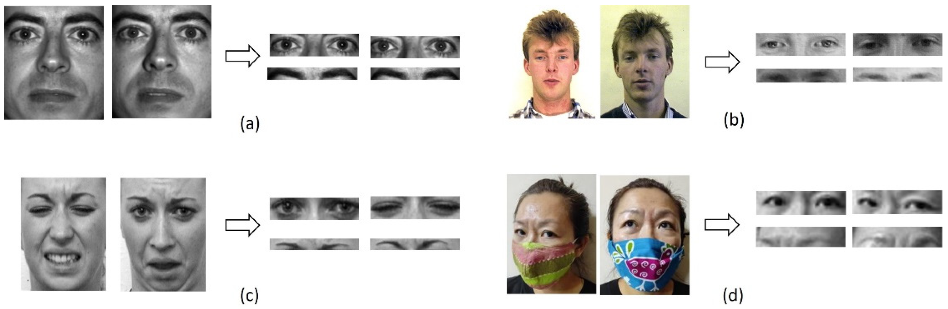
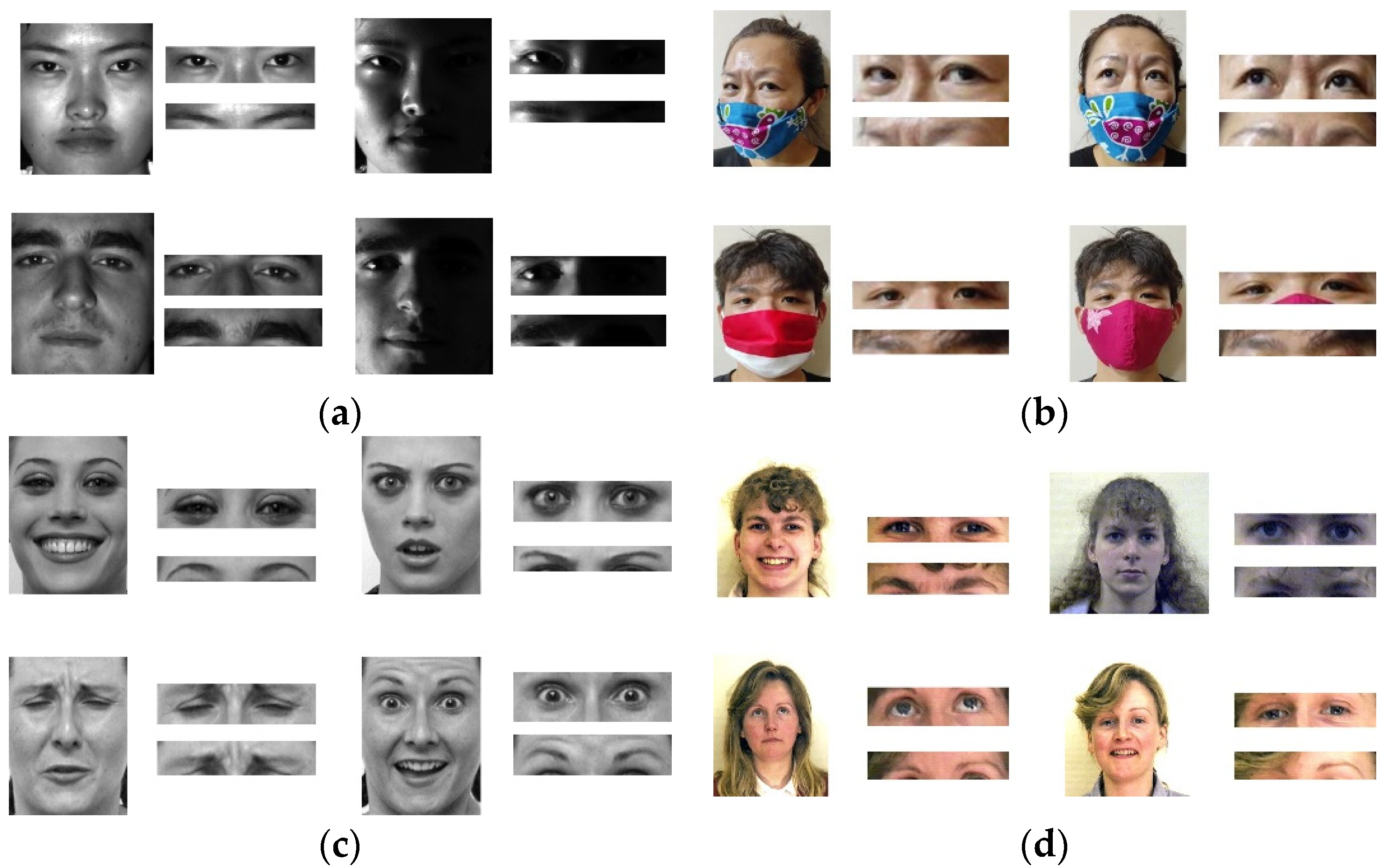
  • The Cropped Extended Yale Face Database B (EYB) [34,35] has 38 frontal face images of 38 respondents in 65 image variations (1 ambient + 62 illuminations). The original size of each image is 168 × 192 pixels in grayscale. Each image in the dataset has little to no variation in the location of the eyes and eyebrows. First, we evaluated 434 cropped face images taken randomly from 7 respondents in the dataset for this research. Since extremely dark images were inside the dataset, we evaluated 62 images for each respondent. We evaluated part of the EYB dataset first to observe the performance of all the proposed ideas. Then, we later re-evaluated the whole dataset using the best method that produced the highest recognition performance to observe the effect using limited data vs. larger data. Re-evaluation for the best method used 2242 images from 38 respondents. A total of 59 images was taken from each respondent. Several images were not observed because they were bad images resulting from the acquisition process.
  • The Aberdeen dataset (ABD) [36] has 687 color face images from 90 respondents. Each respondent provided between 1 and 18 images. The dataset has variations in lighting and viewpoint. The original resolution of this dataset varied from 336 × 480 to 624 × 544 pixels. There are images with different hairstyles, outfits, and facial expressions in the ABD. We evaluated 84 face images randomly from 21 respondents, with a total of 4 images with lighting and viewpoint variations for each respondent. We also re-evaluated the whole dataset to observe the effect using limited data vs. larger data. Re-evaluations for the best method used 244 images from 61 respondents. To create a balanced dataset, we did not use the whole of the images from the 90 respondents because only 61 respondents from the dataset had the consistency of containing 4 images, while the other 29 respondents had a varying number of images per person ranging from 1 to 18 images.
  • The pain expression subset dataset (PES) [36] has 84 cropped images from the pain expression dataset. The face images have a fixed location for the eyes, with 7 expressions from each of the 12 respondents. The original resolution is 181 × 241 pixels in grayscale. The eyes and eyebrows differ in shape according to the respondent’s expression. For this work, we evaluated all images in the dataset.
  • The real fabric face mask dataset (RFFMDS v.1.0) [32] has 176 images from 8 respondents. A total of 22 images consisting of 2 face masks and barefaced images were gathered from each respondent. The images have varying viewpoints and head pose angles. The images are 200 × 150 pixels in an RGB color space. This dataset was evaluated to compare the eye and eyebrow images with full-masked face images for the recognition system. For this dataset, the final size for the cropped eyes image was 49 × 13 pixels, and the final size for the cropped eyebrows image was 67 × 20 pixels. Both the eye and eyebrow images were in grayscale.

2.2.2. Classification and Performance Calculation

The classification process used two methods: k-nearest neighbor (k-NN) and a support vector machine (SVM). The distance metric calculated (d) in k-NN used the Euclidean distance (Equation (24)) [65]. The k-NN method calculates the k-nearest neighbor between two classes of data (testing and training) x and y, respectively. The SVM classifier was tested against the linear kernel (SVM-1) and polynomial kernel (SVM-2):
d ( x , y ) = i = 1 l ( x i y 1 ) 2
Before evaluating the proposed idea against the datasets, we found the best accuracy result with the shortest running time for k-NN was when k = 1. This means we used the single nearest neighbor between the testing and training data. Due to the similar features of the eye images and eyebrow images from different classes (respondents), k = 1 in the k-NN yielded better performance than other values of k. Table 1 displays these preliminary results. These results were evaluated against the eyebrow images using a combination of the scale-space method (O = 0 and L = 2) with the max principal curvature (SS + X).
The images in each dataset were divided in two; the first random half was used for the training data, while the remaining random half was used for validation. We calculated the validation accuracy (Acc) of the recognition system (Equation (25)) for each combination of methods [66]. TP and TN are true positive and true negative, respectively, while FP and FN are false positive and false negative, respectively. The Acc displays how accurately the system recognized individuals:
A c c = T P + T N T P + F P + T N + F N × 100 %
All simulations in this work were compiled using MATLAB Version: 9.10.0.1710957 (R2021a) Update 4 running on an Intel(R) CoreTM) i7-7500U CPU at 2.70 GHz with a 2.90 GHz processor and 16 GB RAM.

3. Results and Discussion

The detailed results of the eye and eyebrow images from the EYB dataset are displayed in Section 3.1 and Section 3.2. The results from the ABD, PES, and RFFMDS v1.0 datasets are compared in Section 3.3. Section 3.4 compares the results from the proposed methods with other works that used the same dataset. We created Table 2 to list the abbreviations used in this research.

3.1. The EYB Eyes Image Results

3.1.1. The Curvature-Based Method Results

This section evaluates the EYB dataset, focusing on the eye images using 1-NN, SVM-1, and SVM-2. Table 3 shows the accuracy results from using the original images (no combination) and the extracted curvature features. The extracted curvatures were the Gaussian curvature (K), mean curvature (H), max principal curvature (X), and min principal curvature (N) from Equations (10)–(12) in Section 2.1. From Table 3, we observed that the extracted curvatures had not improved the performance results. The best accuracy was 66.36%, obtained from SVM-1.

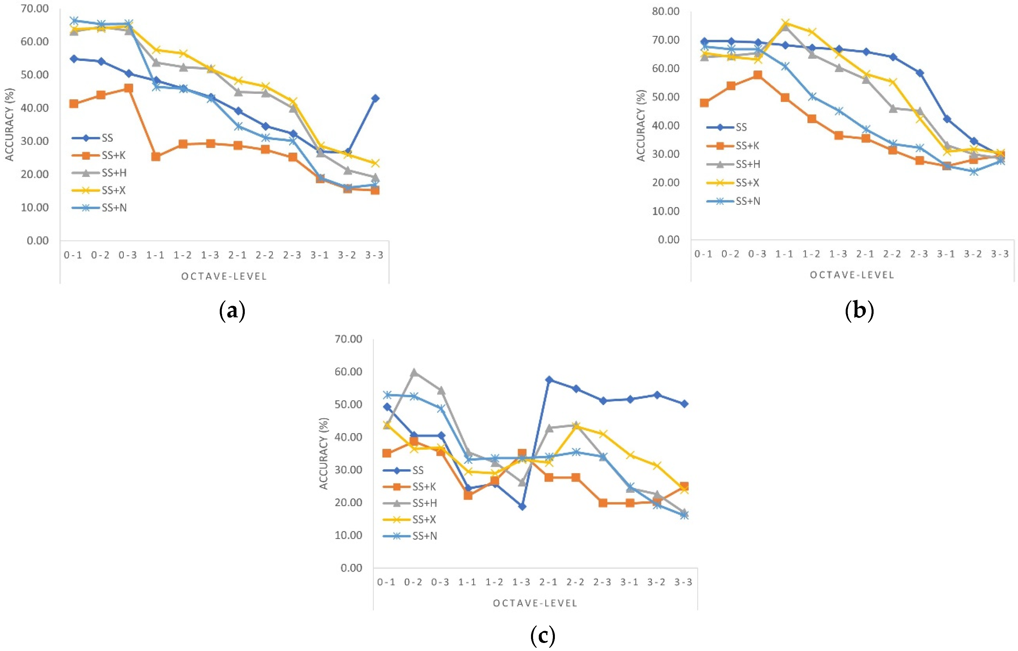
3.1.2. The Scale Space with a Curvature-Based Method Results

In the following experiment, we evaluated the scale-space method from Equations (13) and (17). There were four octaves (O) and three levels in each octave (L). Moreover, the scale space (SS) was then combined with the curvature-based methods in Equations (18)–(20), resulting in a total of 12 variables of O and L from SS and the K, H, X, and N curvatures.
The accuracy results appear in Figure 3. The best results were derived from O = 0 and O = 1, while starting from O = 2, the accuracy results decreased. The performance decreased due to the smaller size of the convoluted images and wider Gaussian width in O = 2 and O = 3. The sizes of the images in O = 1, O = 2, and O = 3 were 59 × 15, 29 × 7, and 14 × 3 pixels, respectively. The widths of the Gaussian filters for L = 1, L = 2, and L = 3 were 1.23, 1.97, and 2.77, respectively.
Consequently, due to the inferior results starting from O = 2, Table 4 displays the results of the curvature-based scale-space method only from O = 0 and O = 1. Overall, the scale space accuracy results from O = 0 performed better than those from O = 1, except for combinations of SS + H (scale space with mean curvature) and SS + X (scale space with the max principal). The results reached the peak at O = 1 and L = 1 from SVM-1. Details from Table 3 also show that SVM-1 produced superior results compared with 1-NN and SVM-2.
We successfully improved the accuracy of the scale-space method by combining it with a curvature-based method. The best accuracies were 76.04% and 74.65%, respectively, from SS + X and SS + H. They improved the previous scale-space method accuracy by 7.84%. Figure 4 shows the results from SS + K, SS + H, SS + X, and SS + N. From Figure 4, we can observe why the combination of SS + H (Figure 4b) and SS + X (Figure 4c) performed well. They were richer in features compared with SS + K (Figure 4a) and SS + N (Figure 4d). The scale space with a curvature-based method effectively captured the prominent feature at O = 1, while the mean and max principal curvature characterized this feature to be more distinctive.

3.1.3. The DWT with a Curvature-Based Method Results

The evaluation of the following experiment used the DWT of the Haar, Sym2, Db2, and Bior2.2 wavelets. There were two decomposition levels with four wavelet coefficients: approximation (A), vertical (V), horizontal (Hr), and diagonal (D) details, as explained in Equation (22).
Table 5 presents the accuracy results for this experiment. The approximation (A) showed the best performances among the other coefficients. The second decomposition level overall displayed higher accuracy results. The results reached the peak performance in A2 (approximation coefficient with the second decomposition level) for all wavelets. The best accuracy result was 72.81% from Sym2 and Db2.
We then observed the results from a combination of the DWT and curvature-based method. Each wavelet coefficient was paired with curvatures in every decomposition level, resulting in 16 variables. Figure 5 shows the results for each classifier. Like the previous results, SVM-1 demonstrated a higher performance accuracy compared with 1-NN and SVM-2. We then further investigated the results using the SVM-1 in Table 6. Table 6 shows that the approximation coefficient produced better results, supporting the previous experiment conclusion from Table 5.
On the other hand, the first decomposition level presented the best results, which is contrary to Table 5, where the second decomposition level produced the best results. The DWT achieved the highest accuracy if paired with H (mean curvature) or X (max principal curvature). This argument supported the previous conclusion in Table 4. The best accuracy result (74.65%) was derived from A-H (approximation with mean curvature) on the first-level decomposition with Sym2 or Db2. The combination of the DWT with the curvature-based method improved the accuracy result by 1.84%.

3.1.4. Summary

This section emphasizes the findings so far based on the results in Section 3.1. First, we found that combining the multiscale analysis methods with the curvature-based methods improved the accuracy results. The improvement varied between 1.84% and 7.84%. Second, we found that the best combination was with the mean curvature and max principal curvature. The highest accuracy was 76.04% from SS + X and 74.05% from SS + H. The mean curvature and the max principal curvature successfully characterized the multiscaled eyes images to be more distinctive. Third, we found that the scale-space method decreased the accuracy when using one-quarter and one-eighth of the resolution of the original image. This decrement also happened in the scale space with the curvature-based method and the DWT with the curvature-based method. On the contrary, the decrement did not happen for the DWT. Fourth, the linear SVM was the best classifier tested against all variables in the whole experiment.

3.2. The EYB Eyebrow Image Results

3.2.1. Curvature-Based Method Results

In this section, an evaluation is performed on the eyebrow images still with the EYB dataset. Table 7 displays the performance results for the eyebrow images using the same experimental conditions for the eye images from Table 3. In contrast to the results from the eye images, from Table 7, we can see that the results from the eyebrow images displayed high accuracy. Almost all combinations with curvatures produced higher results compared with the eye images. The SVM-1 demonstrated superior performance to the original images with the highest accuracy of 92.63% and 91.24% from an extracted min principal curvature (N).

3.2.2. The Scale Space with Curvature-Based Method Results

The same experimental conditions from the eye images in Table 4 were applied to the eyebrow images in this section, resulting in Table 8. The results of the eyebrow images in this experiment also displayed higher performance than the eye images. The conclusion from Table 3 for the accuracy results of O = 0 offered higher accuracy than O = 1, which was also repeated for the eyebrow images.
The highest accuracy result of 94.93% occurred when O = 1 and L = 1 with SS + H. The equal highest accuracy result was also produced with SS + N when O = 0 using SVM-1. The difference between O = 0 and O = 1 was within the Gaussian kernel’s width and the images’ size. In O = 0, the image’s size was bigger than that in O = 1 by half due to the decimation in Equation (17). Figure 6 displays the results from SS + K, SS + H, SS + X, and SS + N. Like the eye images, the combination with H and X resulted in richer features in the eyebrow images. Additionally, for the eyebrow images, the combination with N also performed well.

3.2.3. The DWT with Curvature-Based Method Results

Table 9 displays the results for the eyebrow images using the DWT with the same experimental conditions as the previous eye images from Table 5. The SVM-1 showed consistently superior performance, while overall, the second decomposition level still produced a higher accuracy. Contrary to Table 5, the vertical and horizontal coefficients demonstrated improved results. In several cases (e.g., Hr2 with Sym2 and Db2), the horizontal coefficient displayed a similar or better accuracy than A2 in 1-NN and SVM-1. The best results were obtained from A1 with the Haar wavelet, followed by A1, A2, and Hr2 with Sym2 and Db2. This Hr accentuated the shapes of eyebrows that had more distinctive features in the horizontal direction. Figure 7 displays the DWT results using the Sym2 wavelet with the first decomposition level (Figure 7a) and the second decomposition level (Figure 7b).
Table 10 displays the results of the DWT with a curvature-based method for the eyebrow images. We only presented the results with SVM-1 since this classifier repeatedly showed higher results than 1-NN and SVM-2. The first decomposition level demonstrated higher performance, as shown in Table 6. The curvatures H, X, and N were unsurpassed if combined with the wavelets. Accordingly, the best accuracy was 98.61%, obtained from A-H with the Haar wavelet from the first decomposition level, followed by 98.16% from the Sym2 and Db2 wavelets. This result achieved the highest accuracy thus far. The combination of the DWT with a curvature-based method improved the accuracy result by 6.45%.
Figure 8 displays the results when using the Sym2 wavelet from the first decomposition level’s combined curvature, showing A-K (Figure 8a), A-H (Figure 8b), A-X (Figure 8c), and A-N (Figure 8d). We can observe why A-H, A-X, and A-N performed well, but A-K showed a lesser result. A-K only captured inferior features, which yielded a worse performance in the recognition system.

3.2.4. Summary of the EYB Eyebrow Image Results

The following includes the findings based on Section 3.2. First, we found that the eyebrow images yielded higher accuracy results compared with the eye images. The EYB dataset has variations in the lighting angle. These high results proved the argument in [26] that the eyebrows are robust against illumination. Second, similar to the eye results, the best combination was with the mean curvature and max principal curvature. In addition, in the eyebrow images, the min principal curvature also produced a high accuracy. The highest accuracy was 98.61% from A + H with the Haar wavelet and 98.16% from A + H with the Sym2 and Db2 wavelets. Both were derived using the first decomposition level. The mean, max, and min principal curvatures successfully characterized the multiscale eyebrow images to be more distinctive. Third, we found that the horizontal approximations in the DWT and its combination with a curvature-based method produced high accuracy results. We did not find these high results when using the eye images. The horizontal approximation produced high accuracy because the shape of the eyebrows might have had more distinctive features in the horizontal direction. Fourth, the decreasing results due to the smaller resolutions of the images also happened in the eyebrow images. Fifth, the SVM linear classifier was consistently showing the highest results. This repeated performance also occurred with the eyebrow images.

3.3. Results Using Other Datasets

The best results for the eye images and eyebrow images from the EYB dataset were first re-evaluated using the whole dataset to observe the effect of using the limited number of images vs. larger data. As mentioned before, in this research, the limited data set of EYB contained 434 images from 7 respondents, while the whole EYB dataset contained 2242 images from 38 respondents. The previous best results from the eye images were produced from SS + X and SS + H, while from the eyebrow images, the best results were produced from A + H from the Sym2 and Db2 wavelets.
Table 11 shows the limited data results vs. larger data using the EYB dataset. From Table 11, we observed that by using a larger number of images in the same dataset (EYB dataset), the accuracy results for the eye images showed higher performance, while the eyebrow images showed inferior results. Although the eyebrows feature produced higher performance, the eyes feature in the face images had the potential to be a more stable feature for a larger dataset.
The effects of the limited and whole datasets were also evaluated against the ABD. From Figure 9, we observed that contradictory results were found. The limited ABD produced higher results than the whole ABD for the eye images and eyebrow images. We also assessed the same experimental conditions for the eye and eyebrow images using the PES datasets for the face images and RFFMDS v1.0 for the masked face images. Figure 9 displays the accuracy results from these datasets using SVM-1. We observed that the whole EYB dataset produced the highest accuracy for the eye images, followed by the PES, RFFMDS v1.0, limited EYB, limited ABD, and whole ABD. The limited EYB dataset produced the best results for the eyebrow images, followed by RFFMDS v1.0, whole EYB, PES, limited ABD, and whole ABD. For the limited and whole ABD, the best results were obtained with SS + H at O = 1 and L = 1. In the PES dataset, the best results for the eye images were from A2 with the Sym2 and Db2 wavelets, and the eyebrow images displayed the best results with SS + H at O = 1 and L = 3. For the RFFMDS v1.0 dataset, the best results for the eye images were obtained from SS at O = 0 and L = 3. The eyebrow images displayed the best results from A1 with the Haar wavelet.
It is worth noting the differences between these datasets. The ABD has more variations in showing respondents’ conditions when capturing the images, such as variations in lighting conditions, facial expressions, and hair styles. Sometimes, the hairstyles of the respondents occluded the eye and eyebrow regions. The EYB dataset has little to no variations in the location of the eyes and eyebrows. The variations in the EYB dataset involve poses and illumination. Compared with the EYB dataset, the ABD has more uncontrolled conditions. The PES dataset has variations in respondents’ expressions, resulting in more variations in eye and eyebrow shape, but they have fixed locations. Compared with the ABD, the PES dataset has more controlled conditions. The RFFMDS v1.0 was collected to create a dataset for face images using the actual fabric face mask with random colors and patterns. The variations in the RFFMDS v1.0 involve poses and angles. Our proposed methods were evaluated using this dataset to compare the results of partial face feature recognition with the eyes and eyebrows with full-face features occluded with a face mask. The order of these datasets from controlled to the most uncontrolled conditions was the EYB dataset, the RFFMDS v1.0, the PES dataset, and the ABD. These were in line with the order of the accuracy results in Figure 9. Figure 10 shows the examples of images according to the order of the datasets from controlled to uncontrolled conditions.

3.4. Comparison with Other Methods

In the following section, Table 12 compares the results of our proposed methods with other methods that used the same datasets. We specifically compared RFFMDS v1.0 to contrast the partial face features of the eyes and eyebrows and the masked face images. The best accuracy result from RFFMDS v1.0 [32] was 87.50%, while using the eyebrow images from the same dataset with the proposed method yielded a higher accuracy of 95%. This result demonstrated that the eyebrows could be discriminative enough and employed when other facial parts were occluded.
Using face images from the ABD, Rahmad [67] produced the best accuracy result of 74.83% for an unbalanced dataset using 10-fold cross-validation. Unfortunately, our eye and eyebrow images in this dataset failed to match this result. This poor result was due to more uncontrolled conditions in the ABD that affected the performance of our model. Using face images from the EYB dataset with limited data, our proposed method and idea of using only eyebrow images produced higher results than Yang’s study [68]. Using face images from the whole EYB dataset, Lin [69], Phornchaicharoen [70], Deng [71], and Wright [72] displayed different accuracy results. The highest accuracy was 97.70% from Wright [72], and we successfully achieved a similar accuracy result of 96.88%, but only when using the eye images.

4. Conclusions

We evaluated our proposed methods using the eye and eyebrow images from four face datasets. The combination of the multiscale analysis methods with the curvature-based methods performed well. We achieved the goal from this work, as the scale-space method and discrete wavelet transform successfully exposed details at finer scales, and these details were given in-depth characteristics with a curvature-based method.
Furthermore, the best discriminative features between the eyes and eyebrows were investigated. The variations in the datasets took an important role in the system’s performance. Based on the accuracy results, the eyebrows were suitable for datasets with more controlled conditions, while the eyes were ideal for uncontrolled and larger datasets. The highest accuracy results were 76.04% and 98.61% for the limited dataset, and 96.88% and 93.22% for the larger dataset for the eye and eyebrow images, respectively. The performance results were comparable and achieved similar high accuracy results to other works.

Author Contributions

Conceptualization, R.L.; methodology, D.G.; software, R.L.; validation, C.A. and D.G.; investigation, R.L.; writing—original draft preparation, R.L.; writing—review and editing, C.A.; supervision, C.A. and D.G.; project administration, C.A. All authors have read and agreed to the published version of the manuscript.

Funding

This research is funded by Directorate of Research and Development, Universitas Indonesia under Hibah PUTI 2022 (Grant No. NKB-682/UN2.RST/HKP.05.00/2022).

Institutional Review Board Statement

Not applicable.

Informed Consent Statement

Not applicable.

Data Availability Statement

The datasets which support this article are from the RFFMDS v1.0 data set [32], the cropped extended Yale B dataset [34,35], and the Aberdeen and pain expression subset data sets [36].

Conflicts of Interest

The authors declare no conflict of interest.

References

  1. Peixoto, S.A.; Vasconcelos, F.F.; Guimarães, M.T.; Medeiros, A.G.; Rego, P.A.; Neto, A.V.L.; de Albuquerque, V.H.C.; Filho, P.P.R. A high-efficiency energy and storage approach for IoT applications of facial recognition. Image Vis. Comput. 2020, 96, 103899. [Google Scholar] [CrossRef]
  2. Chen, L.W.; Ho, Y.F.; Tsai, M.F. Instant social networking with startup time minimization based on mobile cloud computing. Sustainability 2018, 10, 1195. [Google Scholar] [CrossRef] [Green Version]
  3. Zeng, D.; Veldhuis, R.; Spreeuwers, L. A survey of face recognition techniques under occlusion. IET Biom. 2021, 10, 581–606. [Google Scholar] [CrossRef]
  4. Zhang, L.; Verma, B.; Tjondronegoro, D.; Chandran, V. Facial expression analysis under partial occlusion: A survey. ACM Comput. Surv. 2018, 51, 1–49. [Google Scholar] [CrossRef] [Green Version]
  5. Damer, N.; Grebe, J.H.; Chen, C.; Boutros, F.; Kirchbuchner, F.; Kuijper, A. The Effect of Wearing a Mask on Face Recognition Performance: An Exploratory Study. In Proceedings of the 2020 International Conference of the Biometrics Special Interest Group (BIOSIG), Darmstadt, Germany, 16–18 September 2020. [Google Scholar]
  6. Carragher, D.J.; Hancock, P.J.B. Surgical face masks impair human face matching performance for familiar and unfamiliar faces. Cogn. Res. Princ. Implic. 2020, 5, 59. [Google Scholar] [CrossRef]
  7. Li, C.; Ge, S.; Zhang, D.; Li, J. Look Through Masks: Towards Masked Face Recognition with De-Occlusion Distillation. In Proceedings of the 28th ACM International Conference on Multimedia, Seattle, WA, USA, 12–16 October 2020. [Google Scholar]
  8. Geng, M.; Peng, P.; Huang, Y.; Tian, Y. Masked Face Recognition with Generative Data Augmentation and Domain Constrained Ranking. In Proceedings of the 28th ACM International Conference on Multimedia, Seattle, WA, USA, 12–16 October 2020. [Google Scholar]
  9. Ding, F.; Peng, P.; Huang, Y.; Geng, M.; Tian, Y. Masked Face Recognition with Latent Part Detection. In Proceedings of the 28th ACM International Conference on Multimedia, Seattle, WA, USA, 12–16 October 2020. [Google Scholar]
  10. Li, Y.; Guo, K.; Lu, Y.; Liu, L. Cropping and attention based approach for masked face recognition. Appl. Intell. 2021, 51, 3012–3025. [Google Scholar] [CrossRef]
  11. Ejaz, M.S.; Islam, M.R. Masked face recognition using convolutional neural network. In Proceedings of the 2019 International Conference on Sustainable Technologies for Industry 4.0 (STI), Dhaka, Bangladesh, 24–25 December 2019. [Google Scholar]
  12. Nguyen, J.; Duong, H. Anatomy, Head and Neck, Anterior, Common Carotid Arteries; StatPearls Publishing: Treasure Island, FL, USA, 2020. [Google Scholar]
  13. Kumari, P.; Seeja, K.R. Periocular biometrics: A survey. J. King Saud Univ. Comput. Inf. Sci. 2019, 34, 1086–1097. [Google Scholar] [CrossRef]
  14. Zhao, Z.; Kumar, A. Improving periocular recognition by explicit attention to critical regions in deep neural network. IEEE Trans. Inf. Forensics Secur. 2018, 13, 2937–2952. [Google Scholar] [CrossRef]
  15. Karczmarek, P.; Pedrycz, W.; Kiersztyn, A.; Rutka, P. A study in facial features saliency in face recognition: An analytic hierarchy process approach. Soft Comput. 2017, 21, 7503–7517. [Google Scholar] [CrossRef] [Green Version]
  16. Peterson, M.F.; Eckstein, M.P. Looking just below the eyes is optimal across face recognition tasks. Proc. Natl. Acad. Sci. USA 2012, 109, E3314–E3323. [Google Scholar] [CrossRef] [Green Version]
  17. Tome, P.; Fierrez, J.; Vera-Rodriguez, R.; Ortega-Garcia, J. Combination of Face Regions in Forensic Scenarios. J. Forensic Sci. 2015, 60, 1046–1051. [Google Scholar] [CrossRef] [PubMed]
  18. Abudarham, N.; Yovel, G. Reverse engineering the face space: Discovering the critical features for face identification. J. Vis. 2016, 16, 40. [Google Scholar] [CrossRef] [PubMed] [Green Version]
  19. Abudarham, N.; Shkiller, L.; Yovel, G. Critical features for face recognition. Cognition 2019, 182, 73–83. [Google Scholar] [CrossRef] [PubMed]
  20. Ding, L.; Martinez, A.M. Features versus context: An approach for precise and detailed detection and delineation of faces and facial features. IEEE Trans. Pattern Anal. Mach. Intell. 2010, 32, 2022–2038. [Google Scholar] [CrossRef] [Green Version]
  21. Biswas, R.; González-Castro, V.; Fidalgo, E.; Alegre, E. A new perceptual hashing method for verification and identity classification of occluded faces. Image Vis. Comput. 2021, 113, 104245. [Google Scholar] [CrossRef]
  22. Wang, Y.; Li, Y.; Song, Y.; Rong, X. Facial expression recognition based on auxiliary models. Algorithms 2019, 12, 227. [Google Scholar] [CrossRef] [Green Version]
  23. Bülthoff, I.; Jung, W.; Armann, R.G.M.; Wallraven, C. Predominance of eyes and surface information for face race categorization. Sci. Rep. 2021, 11, 2021. [Google Scholar] [CrossRef]
  24. Fu, S.; He, H.; Hou, Z.G. Learning race from face: A survey. IEEE Trans. Pattern Anal. Mach. Intell. 2014, 36, 2483–2509. [Google Scholar] [CrossRef] [Green Version]
  25. Oztel, I.; Yolcu, G.; Öz, C.; Kazan, S.; Bunyak, F. iFER: Facial expression recognition using automatically selected geometric eye and eyebrow features. J. Electron. Imaging 2018, 27, 023003. [Google Scholar] [CrossRef]
  26. García-Ramírez, J.; Olvera-López, J.A.; Olmos-Pineda, I.; Martín-Ortíz, M. Mouth and eyebrow segmentation for emotion recognition using interpolated polynomials. J. Intell. Fuzzy Syst. 2018, 34, 3119–3131. [Google Scholar] [CrossRef]
  27. Sadr, J.; Jarudi, I.; Sinha, P. The role of eyebrows in face recognition. Perception 2003, 32, 285–293. [Google Scholar] [CrossRef] [PubMed]
  28. Yujian, L.; Cuihua, F. Eyebrow Recognition: A New Biometric Technique. In Proceedings of the Ninth IASTED International Conference on Signal and Image Processing, Honolulu, HI, USA, 20–22 August 2007. [Google Scholar]
  29. Yujian, L.; Xingli, L. HMM based eyebrow recognition. In Proceedings of the Third International Conference on Intelligent Information Hiding and Multimedia Signal Processing (IIH-MSP 2007), Kaohsiung, Taiwan, 26–28 November 2007. [Google Scholar]
  30. Turkoglu, M.O.; Arican, T. Texture-Based Eyebrow Recognition. In Proceedings of the 2017 International Conference of the Biometrics Special Interest Group (BIOSIG), Darmstadt, Germany, 20–22 September 2017. [Google Scholar]
  31. Li, Y.; Li, H.; Cai, Z. Human eyebrow recognition in the matching-recognizing framework. Comput. Vis. Image Underst. 2013, 117, 170–181. [Google Scholar] [CrossRef]
  32. Lionnie, R.; Apriono, C.; Gunawan, D. Face Mask Recognition with Realistic Fabric Face Mask Data Set: A Combination Using Surface Curvature and GLCM. In Proceedings of the 2021 IEEE International IOT, Electronics and Mechatronics Conference (IEMTRONICS), Toronto, ON, Canada, 21–24 April 2021. [Google Scholar]
  33. Lionnie, R.; Apriono, C.; Gunawan, D. A Study of Orthogonal and Biorthogonal Wavelet Best Basis for Periocular Recognition. ECTI-CIT 2022. submitted. [Google Scholar]
  34. Georghiades, A.S.; Belhumeur, P.N.; Kriegman, D.J. From few to many: Illumination cone models for face recognition under variable lighting and pose. IEEE Trans. Pattern Anal. Mach. Intell. 2001, 23, 643–660. [Google Scholar] [CrossRef] [Green Version]
  35. Lee, K.C.; Ho, J.; Kriegman, D.J. Acquiring linear subspaces for face recognition under variable lighting. IEEE Trans. Pattern Anal. Mach. Intell. 2005, 27, 684–698. [Google Scholar]
  36. Aberdeen, I. Psychological Image Collection at Stirling (PICS). Available online: http://pics.psych.stir.ac.uk/ (accessed on 23 May 2022).
  37. Godinho, R.M.; Spikins, P.; O’Higgins, P. Supraorbital morphology and social dynamics in human evolution. Nat. Ecol. Evol. 2018, 2, 956–961. [Google Scholar] [CrossRef] [Green Version]
  38. Tang, Y.; Li, H.; Sun, X.; Morvan, J.M.; Chen, L. Principal curvature measures estimation and application to 3D face recognition. J. Math. Imaging Vis. 2017, 59, 211–233. [Google Scholar] [CrossRef]
  39. Emambakhsh, M.; Evans, A. Nasal patches and curves for expression-robust 3D face recognition. IEEE Trans. Pattern Anal. Mach. Intell. 2016, 39, 995–1007. [Google Scholar] [CrossRef] [Green Version]
  40. Samad, M.D.; Iftekharuddin, K.M. Frenet frame-based generalized space curve representation for pose-invariant classification and recognition of 3-D face. IEEE Trans. Hum. Mach. Syst. 2016, 46, 522–533. [Google Scholar] [CrossRef]
  41. Bærentzen, J.A. Guide to Computational Geometry Processing; Springer: London, UK, 2012. [Google Scholar]
  42. Callens, S.J.P.; Zadpoor, A.A. From flat sheets to curved geometries: Origami and kirigami approaches. Mater. Today 2018, 21, 241–264. [Google Scholar] [CrossRef]
  43. Gray, A. Modern differential geometry of curves and surfaces with mathematica. Comput. Math. Appl. 1998, 36, 121. [Google Scholar]
  44. Lindeberg, T. Generalized Gaussian Scale-Space Axiomatics Comprising Linear Scale-Space, Affine Scale-Space and Spatio-Temporal Scale-Space. J. Math. Imaging Vis. 2011, 40, 36–81. [Google Scholar] [CrossRef]
  45. Lowe, D.G. Distinctive image features from scale-invariant keypoints. Int. J. Comput. Vis. 2004, 60, 91–110. [Google Scholar] [CrossRef]
  46. Bay, H.; Ess, A.; Tuytelaars, T.; Van Gool, L. Speeded-Up Robust Features (SURF). Comput. Vis. Image Underst. 2008, 110, 346–359. [Google Scholar] [CrossRef]
  47. Burger, W.; Burge, M. Principles of Digital Image Processing: Advanced Methods; Springer Science & Business Media: Berlin/Heidelberg, Germany, 2013. [Google Scholar]
  48. Mokhtarian, F.; Mackworth, A.K. A theory of multiscale, curvature-based shape representation for planar curves. IEEE Trans. Pattern Anal. Mach. Intell. 1992, 14, 789–805. [Google Scholar] [CrossRef]
  49. Mokhtarian, F.; Mackworth, A.K. Scale-Based Description and and recognition of planar curves and two-dimensional shapes. IEEE Trans. Pattern Anal. Mach. Intell. 1986, 8, 34–43. [Google Scholar] [CrossRef] [PubMed] [Green Version]
  50. Hennig, M.; Mertsching, B. Box filtering for real-time curvature scale-space computation. J. Phys. Conf. Ser. 2021, 1958, 012020. [Google Scholar] [CrossRef]
  51. Zeng, J.; Liu, M.; Fu, X.; Gu, R.; Leng, L. Curvature Bag of Words Model for Shape Recognition. IEEE Access 2019, 7, 57163–57171. [Google Scholar] [CrossRef]
  52. Gong, Y.; Goksel, O. Weighted mean curvature. Signal Processing 2019, 164, 329–339. [Google Scholar] [CrossRef]
  53. Tan, W.; Zhou, H.; Song, J.; Li, H.; Yu, Y.; Du, J. Infrared and visible image perceptive fusion through multi-level Gaussian curvature filtering image decomposition. Appl. Opt. 2019, 58, 3064. [Google Scholar] [CrossRef]
  54. Mokhtarian, F.; Suomela, R. Robust image corner detection through curvature scale space. IEEE Trans. Pattern Anal. Mach. Intell. 1998, 20, 1376–1381. [Google Scholar] [CrossRef] [Green Version]
  55. Bakar, S.A.; Hitam, M.S.; Yussof, W.N.J.H.W.; Mukta, M.Y. Shape Corner Detection through Enhanced Curvature Properties. In Proceedings of the 2020 Emerging Technology in Computing, Communication and Electronics (ETCCE), Dhaka, Bangladesh, 21–22 December 2020. [Google Scholar]
  56. Sundararajan, D. Discrete Wavelet Transform: A Signal Processing Approach; John Wiley & Sons: Hoboken, NJ, USA, 2015. [Google Scholar]
  57. Xu, W.; Ding, K.; Liu, J.; Cao, M.; Radzieński, M.; Ostachowicz, W. Non-uniform crack identification in plate-like structures using wavelet 2D modal curvature under noisy conditions. Mech. Syst. Signal Processing 2019, 126, 469–489. [Google Scholar] [CrossRef]
  58. Janeliukstis, R.; Rucevskis, S.; Wesolowski, M.; Chate, A. Experimental structural damage localization in beam structure using spatial continuous wavelet transform and mode shape curvature methods. Measurement 2017, 102, 253–270. [Google Scholar] [CrossRef]
  59. Bao, L.; Cao, Y.; Zhang, X. Intelligent Identification of Structural Damage Based on the Curvature Mode and Wavelet Analysis Theory. Adv. Civ. Eng. 2021, 2021, 8847524. [Google Scholar] [CrossRef]
  60. Teimoori, T.; Mahmoudi, M. Damage detection in connections of steel moment resisting frames using proper orthogonal decomposition and wavelet transform. Measurement 2020, 166, 108188. [Google Scholar] [CrossRef]
  61. Karami, V.; Chenaghlou, M.R.; Gharabaghi, A.R.M. A combination of wavelet packet energy curvature difference and Richardson extrapolation for structural damage detection. Appl. Ocean Res. 2020, 101, 102224. [Google Scholar] [CrossRef]
  62. Zhang, X.; Wu, J.; Meng, M. Small Target Recognition Using Dynamic Time Warping and Visual Attention. Comput. J. 2020, 65, 203–216. [Google Scholar] [CrossRef]
  63. Li, J.; Ma, H.; Lv, Y.; Zhao, D.; Liu, Y. Finger vein feature extraction based on improved maximum curvature description. In Proceedings of the 2019 Chinese Control Conference (CCC), Guangzhou, China, 27–30 July 2019. [Google Scholar]
  64. Viola, P.; Jones, M. Robust real-time face detection. Int. J. Comput. Vis. 2004, 57, 137–154. [Google Scholar] [CrossRef]
  65. Patel, S.P.; Upadhyay, S.H. Euclidean distance based feature ranking and subset selection for bearing fault diagnosis. Expert Syst. Appl. 2020, 154, 113400. [Google Scholar] [CrossRef]
  66. Powers, D. Evaluation: From Precision, Recall and F-Measure to ROC, Informedness, Markedness & Correlation. J. Mach. Learn. Technol. 2011, 2, 37–63. [Google Scholar]
  67. Rahmad, C.; Arai, K.; Asmara, R.A.; Ekojono, E.; Putra, D.R.H. Comparison of Geometric Features and Color Features for Face Recognition. Int. J. Intell. Eng. Syst. 2021, 14, 541–551. [Google Scholar] [CrossRef]
  68. Huixian, Y.; Gan, W.; Chen, F.; Zeng, J. Cropped and Extended Patch Collaborative Representation Face Recognition for a Single Sample Per Person. Autom. Control Comput. Sci. 2019, 53, 550–559. [Google Scholar] [CrossRef]
  69. Lin, J.; Te Chiu, C. Low-complexity face recognition using contour-based binary descriptor. IET Image Process. 2017, 11, 1179–1187. [Google Scholar] [CrossRef]
  70. Phornchaicharoen, A.; Padungweang, P. Face recognition using transferred deep learning for feature extraction. In Proceedings of the 2019 Joint International Conference on Digital Arts, Media and Technology with ECTI Northern Section Conference on Electrical, Electronics, Computer and Telecommunications Engineering (ECTI DAMT-NCON), Nan, Thailand, 30 January–2 February 2019. [Google Scholar]
  71. Deng, W.; Hu, J.; Guo, J. Face Recognition via Collaborative Representation: Its Discriminant Nature and Superposed Representation. IEEE Trans. Pattern Anal. Mach. Intell. 2018, 40, 2513–2521. [Google Scholar] [CrossRef] [PubMed]
  72. Wright, J.; Yang, A.Y.; Ganesh, A.; Sastry, S.S.; Ma, Y. Robust Face Recognition via Sparse Representation. IEEE Trans. Pattern Anal. Mach. Intell. 2009, 31, 210–227. [Google Scholar] [CrossRef] [Green Version]
Figure 1. The overall flowchart of the proposed idea. Connectors A, B, and C detail the curvature-based, scale-space, and discrete wavelet transform processes.
Algorithms 15 00208 g001aAlgorithms 15 00208 g001b
Figure 2. Example of face images from datasets and cropped results for eye and eyebrow images: (a) EYB, (b) ABD, (c) PES, and (d) RFFMDS v1.0.
Algorithms 15 00208 g002
Figure 3. The accuracy results (%) from (a) 1-NN, (b) SVM-1, and (c) SVM-2. The results were evaluated for 12 octave O and level L variables from SS and 5 curvature-based scale spaces (SS, SS + K, SS + H, SS + X, and SS + N).
Algorithms 15 00208 g003
Figure 4. Combination results for (a) SS + K, (b) SS + H, (c) SS + X, and (d) SS + N with O = 1 and L = 1 on an eye image.
Algorithms 15 00208 g004
Figure 5. The accuracy results (%) from (a) 1-NN, (b) SVM-1, and (c) SVM-2. The results were evaluated for a total of 16 variables for wavelet coefficients (A, V, Hr, and D) with 2 decomposition levels and curvature-based methods (K, H, X, and N).
Algorithms 15 00208 g005
Figure 6. Combination results of (a) SS + K, (b) SS + H, (c) SS + X, and (d) SS + N with O = 1 and L = 1 for an eyebrow image.
Algorithms 15 00208 g006
Figure 7. Sym2 wavelet coefficients on an eyebrow image with (a) the first decomposition level and (b) the second decomposition level.
Algorithms 15 00208 g007
Figure 8. Sym2 wavelet from the first decomposition level combined with curvature-based method: (a) A-K, (b) A-H, (c) A-X, and (d) A-N.
Algorithms 15 00208 g008
Figure 9. Accuracy results (%) from EYB, ABD, PES, and RFFMDS v1.0 datasets for eye images and eyebrow images.
Algorithms 15 00208 g009
Figure 10. Examples of images according to the order of the datasets from controlled to uncontrolled conditions: (a) EYB dataset, (b) RFFMDS v1.0, (c) PES dataset, and (d) ABD.
Algorithms 15 00208 g010
Table 1. The accuracy (%) results and training time (s) of the eyebrow images using SS + X with O = 0 and L = 2 with its respective value of k in the k-NN classifier.
k-NNAcc (%)Training Time (s)
k = 191.0013.47
k = 389.2017.02
k = 585.5017.31
k = 784.1014.69
Table 2. The list of abbreviations in this research.
Abbr.Method
KGaussian curvature
Hmean curvature
Xmax principal curvature
Nmin principal curvature
SS + K/H/X/Nscale space with curvature (Gaussian, mean, max principal, and min principal)
O-Loctave level in scale space
A#approximation coefficient in DWT from # (decomposition level)
Hr#horizontal coefficient in DWT from # (decomposition level)
V#vertical coefficient in DWT from # (decomposition level)
D#diagonal coefficient in DWT from # (decomposition level)
Sym2Symlet wavelet with 2 vanishing moments
Db2Daubechies wavelet with 2 vanishing moments
Bior2.2biorthogonal wavelet with 2 vanishing moments for synthesis and analysis
1-NNk-nearest neighbor with k = 1
SVM-1support vector machine with linear kernel
SVM-2support vector machine with polynomial kernel
Table 3. The accuracy (%) results from the EYB dataset for the eye images and the extracted curvatures.
ClassificationBaseCurvature-Based
KHXN
1-NN58.9215.8832.5847.4251.36
SVM-166.3631.8051.6159.9158.99
SVM-244.7025.8130.4134.5622.12
Table 4. The detailed accuracy (%) results of the scale-space method and its combination with a curvature-based method (SS, SS + K, SS + H, SS + X, and SS + N) on EYB dataset for the eye images.
ClassifierMethodOctave-Level (O-L)
0-10-20-31-11-21-3
1-NNSS54.8454.1050.4148.3645.9043.32
SS + K41.2443.8945.9025.3229.1029.29
SS + H63.2064.4963.3253.7852.3551.89
SS + X63.8564.0664.7057.5856.4351.77
SS + N66.4165.3565.4646.3845.8842.86
SVM-1SS69.5969.5969.1268.2067.2866.82
SS + K47.9353.9257.6049.7742.4036.41
SS + H64.0664.5265.4474.6564.9860.37
SS + X65.4464.0663.1376.0472.8164.98
SS + N67.7466.8266.8260.8350.2345.16
SVM-2SS49.3140.5540.5524.4225.8118.89
SS + K35.0238.7135.4822.1226.7335.02
SS + H43.7859.9154.3835.4832.2626.27
SS + X43.7836.4136.8729.4929.0333.18
SS + N53.0052.5348.8533.1833.6433.64
Table 5. The accuracy (%) results of the DWT on the EYB dataset for the eye images. The performance was calculated for all wavelet coefficients in two decomposition levels, producing A1, V1, Hr1, D1, A1, V2, Hr2, and D2.
ClassifierDWTWavelet Coefficient and Decomposition Level
A1V1Hr1D1A2V2Hr2D2
1-NNHaar58.0650.7151.6420.07 55.4458.8756.8729.82
Sym259.4521.0632.7014.4058.2945.8552.1722.24
Db259.2921.0832.8614.8258.0445.5551.7122.33
Bior2.257.2418.3927.6014.9558.2731.2443.8017.65
SVM-1Haar67.2858.0655.3041.9470.5156.6854.3843.32
Sym266.3641.4748.8530.8872.8147.0051.1527.19
Db266.3641.4748.8530.8872.8147.0051.1527.19
Bior2.269.1240.5547.0026.2771.4339.1742.8623.50
SVM-2Haar16.1333.1836.8730.4156.6844.2437.3329.03
Sym216.5924.4229.9526.2751.6135.0243.7827.19
Db216.5924.4229.9526.2751.6135.0243.7827.19
Bior2.220.7428.1128.5720.7441.4726.7329.9523.96
Table 6. The detailed accuracy (%) results of the combined DWT with a curvature-based method on the EYB dataset for the eye images using SVM-1. The combined methods produced wavelet coefficients with two decomposition levels and curvature-based variables (e.g., A-K (approximation with Gaussian curvature) until D-N (diagonal with min principal curvature)).
ClassifierDWTWavelet Coefficient and Curvature Combination
A-KA-HA-XA-NV-KV-HV-XV-NHr-KHr-HHr-XHr-ND-KD-HD-XD-N
SVM-1Haar Lv120.2870.5164.0656.2221.6651.6144.2447.4722.1253.9251.1550.6924.8843.7838.2539.63
Haar Lv228.1161.7565.4455.7625.3552.0741.0145.6220.7448.8546.0848.8521.6634.5631.8030.41
Sym2 Lv122.5874.6564.0669.1222.5846.5444.2443.7826.7345.1638.7142.4029.9528.5737.3332.72
Sym2 Lv228.1166.3668.6658.9917.0543.7834.1040.0921.6647.4742.4040.0917.0523.5024.4231.34
Db2 Lv122.5874.6564.0669.1222.5846.5444.2443.7826.7345.1638.7142.4029.9528.5737.3332.72
Db2 Lv228.1166.3668.6658.9917.0543.7834.1040.0921.6647.4742.4040.0917.0523.5024.4231.34
Bior2.2 Lv123.5070.9765.9068.6622.5844.7044.2438.2525.3545.1646.0841.0126.2725.8132.7235.48
Bior2.2 Lv230.4164.5265.9059.9119.8241.4735.9436.4123.9639.1739.1740.0922.1223.9630.4128.57
Table 7. The accuracy (%) results from the EYB dataset for the eyebrow images and the extracted curvatures.
ClassifierBaseCurvature-Based
KHXN
1-NN63.2718.2952.6572.7472.86
SVM-192.6356.6886.6486.6491.24
SVM-264.5235.9447.9331.3435.94
Table 8. The detailed accuracy (%) results of the scale-space method and its combination with a curvature-based method (SS, SS + K, SS + H, SS + X, and SS + N) on the EYB dataset for the eyebrow images.
ClassifierMethodOctave-Level (O-L)
0-10-20-31-11-21-3
1-NNSS57.7656.3655.3052.2449.9545.18
SS + K47.7448.1639.5235.3738.6937.35
SS + H82.7083.1183.2576.8276.0470.90
SS + X83.7691.0083.4169.1264.8861.45
SS + N84.2283.0082.5379.2674.7267.12
SVM-1SS87.5688.4887.1085.2586.6486.18
SS + K78.8082.9583.8764.5265.4465.44
SS + H93.5594.4789.8694.9393.5585.71
SS + X94.0193.0991.2488.9488.4882.03
SS + N93.5594.9393.0993.5589.4083.41
SVM-2SS66.3647.4755.3029.4922.5823.04
SS + K36.8739.6344.7021.2034.1023.50
SS + H63.5957.1438.2531.3432.2633.64
SS + X46.0867.7430.4128.1127.1922.12
SS + N62.2155.7657.6038.7140.0933.64
Table 9. The accuracy (%) results of the DWT on the EYB dataset for the eyebrow images. The performance was calculated for all wavelet coefficients in two decomposition levels, producing A1, V1, Hr1, D1, A1, V2, Hr2, and D2.
ClassifierDWTWavelet Coefficient and Decomposition Level
A1V1Hr1D1A2V2Hr2D2
1-NNHaar63.6960.5877.6524.2961.5278.0277.5133.34
Sym262.7630.1656.4717.1459.0363.2981.1333.06
Db263.0229.2652.6717.1060.0057.9381.5034.06
Bior2.264.0325.5346.3817.2662.2646.9675.2325.46
SVM-1Haar92.1784.7987.179.7289.486.1886.1869.12
Sym291.7173.7383.4174.6591.7186.6491.2470.97
Db291.7173.7383.4174.6591.7186.6491.2470.97
Bior2.291.7176.9683.8769.5990.7880.1887.5657.6
SVM-2Haar35.4843.3240.5534.5660.8356.2248.3932.26
Sym226.7336.8735.0223.9659.4541.4745.6235.02
Db226.7336.8735.0223.9659.4541.4745.6235.02
Bior2.229.0337.7935.9431.856.6832.2644.2429.49
Table 10. The accuracy (%) results of combined DWT with a curvature-based method on the EYB dataset for the eyebrow images using SVM-1. The combined methods produced wavelet coefficients with two decomposition levels and curvature-based variables (e.g., A-K (approximation with Gaussian curvature) until D-N (diagonal with min principal curvature)).
ClassifierDWTWavelet Coefficient and Curvature Combination
A-KA-HA-XA-NV-KV-HV-XV-NHr-KHr-HHr-XHr-ND-KD-HD-XD-N
SVM-1Haar Lv138.2598.6195.3996.7737.7990.7887.5689.8640.0992.6392.6391.7147.9380.6582.9582.95
Haar Lv234.1088.4882.9587.5633.6492.1782.4988.0230.8890.7889.8684.7927.1971.4359.9165.44
Sym2 Lv143.7898.1696.3197.2443.3288.4884.7985.2542.4094.0194.0191.2448.3972.8176.9669.59
Sym2 Lv241.9494.0186.6494.9330.4182.0384.3381.1135.9492.6388.9492.6327.1970.9760.3765.90
Db2 Lv143.7898.1696.3197.2443.3288.4884.7985.2542.4094.0194.0191.2448.3972.8176.9669.59
Db2 Lv241.9494.0186.6494.9330.4182.0384.3381.1135.9492.6388.9492.6327.1970.9760.3765.90
Bior2.2 Lv134.5696.7796.7797.2440.0987.1079.2683.4135.9493.0990.7893.0944.7068.2070.9767.74
Bior2.2 Lv234.5693.0989.4094.0129.4972.8167.2869.1232.7290.7890.3287.1026.7352.0749.7751.61
Table 11. The accuracy (%) results of the limited EYB dataset vs. the whole EYB dataset against the best method in all proposed idea.
RegionMethodAccuracy (%)
Limited EYB (434 Images)Whole EYB (2242 Images)
Eyesbase66.3674.04
SS + H74.6585.37
SS + X76.0483.41
Sym2(A) + H74.6596.88
Sym2(A) + X64.0696.52
Db2(A) + H74.6596.88
Db2(A) + X64.0696.52
Eyebrowsbase92.6379.3
SS + H94.9383.23
SS + N94.9383.59
Sym2(A) + H98.1683.59
Sym2(A) + X96.3193.22
Db2(A) + H98.1683.59
Db2(A) + X96.3193.22
Table 12. Comparison of accuracy (%) results with other methods.
DatasetMethodsAccuracy (%)Total Images (Class/Testing per Class/Training per Class)
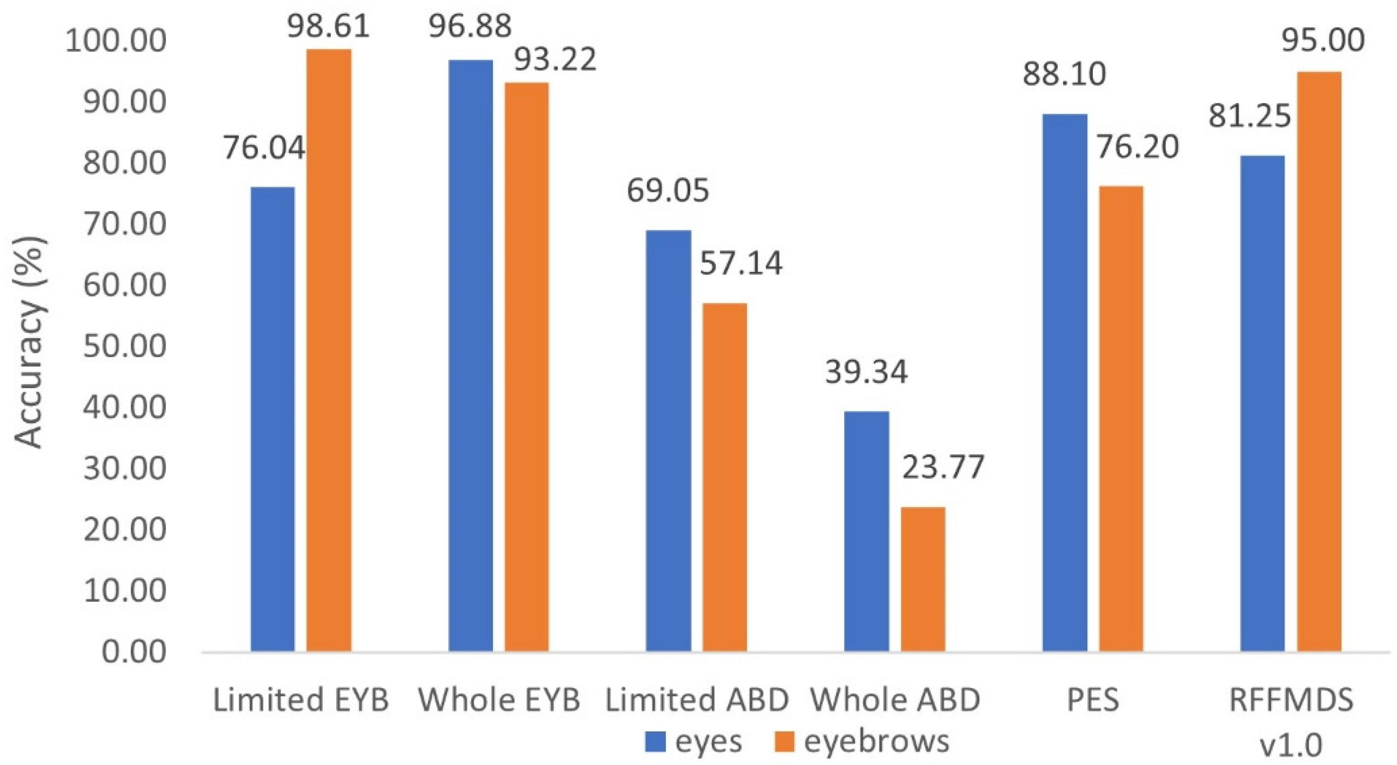
RFFMDS v1.0Eyes *81.25160 (8/10/10)
Eyebrows *95.00160 (8/10/10)
Lionnie [32]87.50176 (8/2/20)
ABDEyes *69.0584 (21/2/2)
Eyebrows *57.1484 (21/2/2)
Eyes *39.34244 (61/2/2)
Eyebrows *23.77244 (61/2/2)
Rahmad [67] on SVM74.83687 (90:10-CV) **
EYB datasetEyes *76.04434 (7/31/31)
Eyebrows *98.61434 (7/31/31)
Eyes *96.882242 (38/29/30)
Eyebrows *93.222242 (38/29/30)
Yang [68]93.9670 (10/1/6)
Lin [69]67.422432 (38/1/63)
Phornchaicharoen [70]96.562404 (80:20) ***
Deng [71] on L-SVM97.102432 (38/32/32)
Wright [72] on SVM97.702432 (38/32/32)
* Results from the proposed methods. ** On 90/10 training/testing cross-validation total of 687 images with unbalanced dataset. *** On 80/20 training/testing division for 2404 images.
Publisher’s Note: MDPI stays neutral with regard to jurisdictional claims in published maps and institutional affiliations.

