Article

Improving the Quantum Multi-Swarm Optimization with Adaptive Differential Evolution for Dynamic Environments

1
Department of System Analysis and Operations Research, Reshetnev Siberian State University of Science and Technology, 660037 Krasnoyarsk, Russia
2
Heuristic and Evolutionary Algorithms Laboratory, University of Applied Sciences Upper Austria, Softwarepark 11, 4232 Hagenberg, Austria
*
Author to whom correspondence should be addressed.
Algorithms 2022, 15(5), 154; https://doi.org/10.3390/a15050154
Submission received: 29 March 2022 / Revised: 28 April 2022 / Accepted: 28 April 2022 / Published: 30 April 2022
(This article belongs to the Special Issue Mathematical Models and Their Applications III)

Abstract

:
In this study, the modification of the quantum multi-swarm optimization algorithm is proposed for dynamic optimization problems. The modification implies using the search operators from differential evolution algorithm with a certain probability within particle swarm optimization to improve the algorithm’s search capabilities in dynamically changing environments. For algorithm testing, the Generalized Moving Peaks Benchmark was used. The experiments were performed for four benchmark settings, and the sensitivity analysis to the main parameters of algorithms is performed. It is shown that applying the mutation operator from differential evolution to the personal best positions of the particles allows for improving the algorithm performance.

1. Introduction

The development of computational intelligence approaches has allowed applying these methods in different areas nowadays. In particular, the evolutionary computation (EC) [1] methods and swarm-based algorithms proved themselves to be problem-independent and universal approaches for solving optimization tasks with different types of complexity. Most of these algorithms are developed to address stationary environments, where the objective function does not change over time. However, optimization in dynamic environments has become popular in the last three decades, which is indicated in several surveys of the state-of-the-art [2,3,4]. Many real-world applications can be formulated as a dynamic optimization problem (DOP), where the problem itself changes over time. The changing environment during the optimization process is a challenging task for most bio-inspired algorithms, as they are mainly developed under an assumption that a single best final solution should be found by the end of the computational resource, and the goal function does not change.
In the non-stationary environment, the goal consists in tracking the optimum positions during the optimization process. The problems which are formulated as DOPs, are found in different areas of human activity such as path planning [4,5], pollution control [6], searching for survivors with unmanned aerial vehicles (drones) [7], and others. The development of novel approaches for DOPs relies on well-established benchmarks, namely the classical Moving Peaks Benchmark (MPB) [8], Generalized Dynamic Benchmark Generator (GDBG) [9], or the recently proposed Generalized Moving Peaks Benchmark (GMPB) [10,11] and the Deterministic Distortion and Rotation Benchmark (DDRB) [12].
The dominating methods often applied for DOPs are the particle swarm optimization (PSO)-based algorithms and their modifications such as multi-swarm approaches [13,14], however, certain studies used Differential Evolution (DE) [15] or, for example, Artificial Bee Colony (ABC) algorithm [16]. Yet little has been done for the development of hybrid approaches, which would use the advantages of different methods. Thus, the goal of this study is to establish the ways in which DE can be added to PSO-based approaches, improving the resulting performance.
In this study, the multi-swarm Quantum Swarm Optimization (mQSO) [13] algorithm is modified with the Differential Evolution search operator. Several versions of the resulting mQSODE algorithm with different mutation operators are considered, and the sensitivity analysis for main parameters is conducted. The experiments are performed on the Generalized Moving Peaks Benchmark [10] with four scenarios. The main contributions of the current study can be summarized as follows:
  • It is shown that applying differential mutation to current positions of the particles is inferior to the variant when it is applied to personal best positions;
  • The probability of applying differential evolution search should be relatively small, and the PSO should be the main search engine to achieve competitive results;
  • The scaling factor in differential mutation should be carefully chosen, as it significantly influences performance, whereas crossover rate does not seem to have any significant influence;
  • Applying differential mutation with a small probability results in higher diversity in the population compared to mQSO given the same population size;
  • The GMPB favors larger population sizes than recommended values, derived from testing on other benchmarks.
The rest of the paper is organized as follows: the next section describes related work, i.e., algorithms and methods applied to dynamic optimization, after this the generalized moving peaks benchmark used in this study is given, next, the proposed approach is presented, after that, the experimental setup and results are provided, and finally, the conclusions are given.

2. Materials and Methods

2.1. Related Work

Without loss of generality, we can state the classic unconstrained single-objective continuous DOP as follows.
o p t i m i z e   f ( x ¯ , φ ¯ , t ) ,   x ¯ F ( t ) S , t T
where S R d , d is the search space dimensionality, S is the search space, t denotes the time, φ ¯ is the set of parameters of the current environment, f : S × T R , is the objective function that returns a value ( f ( x ¯ , φ ¯ , t ) )   R using the feasible solution from the search space at time t, F ( t ) —is a set of feasible solutions at time t .
There are a lot of approaches that have been proposed to handle DOPs, some of them are described below:
  • Detection-based approaches. This group of methods can be divided into two subcategories: a solution reevaluation [8,17] and detection changes in an algorithm’s behavior [18,19]. The solution reevaluation is based on the reevaluation of some solution at a given frequency. If the fitness value of this solution is changed, then the environment is changed too. The second way is based on monitoring the drop in the average performance of an algorithm over several generations. Additionally, some algorithms evaluate the diversity of fitness values.
  • Introducing diversity when changes are detected. When solving the stationary optimization problem, the population has to converge to an optimum. When solving DOP, if the whole population is converged to some optimum and the environment is changed, the algorithm cannot react to the change quickly and effectively. The following approach has been proposed to diversify the population. In [18], a partial hypermutation step has been proposed. It replaces a predefined percentage of individuals, generated randomly from the feasible search space. The proposed genetic programming approach [19] increases the mutation factor, reduces elitism, and increases the probability of crossover when the environment is changed.
  • Maintaining diversity during the search. Methods from this group do not detect directly when the environment is changed. They are based on keeping the diversity of the population on the same level. In the random immigrants method [20], a predefined number of randomly generated individuals are added to the population in every generation. The sentinel placement method [21] initializes the predefined number of points that cover the search space. Authors use the proposed method to cover the search space more uniformly.
  • Memory approaches. If the changes in the environment are periodical, i.e., the landscape of the problem can return, it is useful to contain previous solutions to save computational resources. The previous good solutions are stored in a direct memory [22,23].
  • Prediction approaches. In this case, a heuristic tries to find some patterns that are predictable and use this information to increase the search performance when the environment is changed. A prediction of the optima movement is described in [24]. The prediction model is based on a sequence of optimum positions found in the previous environments.
  • Multi-population approaches. The idea of the approach is to share responsibilities between populations. For example, the first population may focus on searching for the optimum while the second population focuses on tracking any environmental changes. The approach [25] uses the predefined number of small populations to find better solutions and one big population to track changes. Another method [26] uses the main big population to optimize the current environment and dedicates some small populations to track the changes in the environment.
Most of the modern approaches utilize the multi-population concept, for example, in [27], a general adaptive multi-swarm framework is proposed, in which the number of swarms is dynamically adapted and some of the swarms are set to an inactive state to save computational resource. In the AMP framework proposed in [28], several heuristics are applied, including population exclusion, avoidance of explored peaks, population hibernation and wakening, as well as the Brownian movement.
Other studies, such as [29] or [30], propose the use of clustering methods for dividing the population into sub-swarms, and depending on a threshold condition, close swarms could be merged into one. In some papers, such as [31,32] it was shown that the idea of having multiple dynamic swarms could be efficiently applied also to static test suites such as the well-known Congress on Evolutionary Computation competition problems [33], real-world problems, such as energy consumption optimization [34] or constrained optimization problems [35].
Although there is a certain amount of studies on dynamic optimization, which use DE-based algorithms, such as DynPopDE [15], most of them are focused on PSO due to its simplicity and ability to converge fast. However, in stationary environments, hybrid approaches are well-known, for example, in [36], a hybrid algorithm is applied to the optimal design of water distribution systems, in [37], the algorithm with repulsive strategy is proposed, and in [38], the soft island model with different types of populations is proposed. Considering these studies, the development of hybrid approaches combining PSO and DE could be a promising research direction.

2.2. Generalized Moving Peaks Benchmark

As mentioned before, real-world dynamic optimization problems have complex landscapes and, therefore, algorithms applied to them have to be able to find desirable solutions while also reacting to the environmental changes. The latter is important due to the fact that these changes cause the shift of the optimal solution, namely, the previously found solution becomes suboptimal and the new one should be found for a current environment. Thus, in order to evaluate the performance of the proposed algorithms, it is crucial to use benchmark problems that can be described by the following features:
  • Easy implementation;
  • High configurability with respect to the number of components, the shape of components, dimension, environmental change frequency, and severity;
  • Variety of characteristics (modularity, components with different condition numbers, different intensity of local and global modality, heterogeneity, different levels of irregularities, symmetric and asymmetric components, and so on).
One of the most popular and well-known generators for DOP benchmarks is the Moving Peaks Benchmark (MPB) [8], which is based on changing the components and their locations over time. However, this benchmark generator cannot be considered useful or practical due to its irrelevance to real-world problems. Therefore, the Generalized Moving Peaks Benchmark (GMPB) generator was later proposed [10]. GMPB is a benchmark generator with fully controllable features: it is capable of generating problems with fully non-separable to fully separable structure, with homogeneous or highly heterogeneous, balanced or highly imbalanced sub-functions, with unimodal or multimodal, symmetric or asymmetric and smooth or highly irregular components.
The GMPB benchmark generator, introduced in [10], has the following baseline function:
f ( t ) ( x ) = max k { 1 , , m } { h k ( t ) T ( ( x c k ( t ) ) T R k ( t ) T , k ) W k ( t ) T ( R k ( t ) ( x c k ( t ) ) T , k ) }
T ( y j , k ) = { e x p ( l o g ( y j ) + τ k ( t ) ( s i n ( η k , 1 ( t ) l o g ( y j ) ) + s i n ( η k , 2 ( t ) l o g ( y j ) ) ) ) ,   y j > 0 0 ,   y j = 0 e x p ( l o g ( | y j | ) + τ k ( t ) ( s i n ( η k , 3 ( t ) l o g ( | y j | ) ) + s i n ( η k , 4 ( t ) l o g ( | y j | ) ) ) ) ,   y j > 0 j = 1 , d ¯
In these formulas the following notations are used: x is a solution vector, d is the number of dimensions, m is the number of components, c k ( t ) is the vector of center positions of the k -th component at time t , R k ( t ) is the rotational matrix of component k in the environment t, W k ( t ) is a width matrix (it is a d × d diagonal matrix where each diagonal element is the width of the component k), and, finally, η k , l ( t ) , l = 1 , 4 ¯ , and τ k ( t ) are the irregularity parameters of the component k. Here, for each component, the height, width, irregularity, and all other parameters change as soon as the environmental change happens.
The mentioned function (1) can be used with basic parameters, thus, in the simplest form: in the case where the generated DOP would be symmetric, unimodal, and smooth, the result would be easily optimized. To make the generated problems more complex, the irregularity parameters η k , l ( t ) and τ k ( t ) should be changed. By setting different values to those parameters the end-user can get irregular and/or multimodal optimization tasks.
The higher values of the irregularity parameters ( η k , l ( t ) and τ k ( t ) ) increase the number of local optima in a given peak. It should be noted that identical values of the irregularity parameters η k , l ( t ) lead to the symmetric DOPs, while the components with different η k , l ( t ) values are asymmetric. Additionally, each component’s intensity of irregularities, number of local optima, and asymmetry degree change over time due to the fact that parameters η k , l ( t ) and τ k ( t ) change over time.
The rotation matrix R k ( t ) is obtained for each component k by rotating the projection of solution x onto all existing unique planes of the search space by a given angle. For that purpose, a Givens rotation matrix is constructed, which is firstly initialized as an identity matrix and then altered. Besides, it should be noted that the initial rotation matrix is obtained by using the Gram-Schmidt orthogonalization method on a matrix with normally distributed entries.
For DOPs obtained by the MPB generator, the width of each component or peak is, in other words, the same in all dimensions, therefore, the shape of components is cone-like with circular contour lines. It was changed for the GMPB benchmark generator, namely, each peak’s width was changed from a scalar variable to a vector with d dimensions. Thus, a component generated by GMPB has a width value in each dimension.
The condition number of a component is the ratio of its largest width value to its smallest value, and if a component’s width value is stretched in one axis’s direction more than the other axes, then, the component is ill-conditioned. As result, the ill-conditioning degree of each component can be determined by calculating the condition number of the diagonal matrix W k ( t ) . So, the GMPB generator, unlike the MPB generator, is capable of creating components with various condition numbers, i.e., it can additionally generate ill-conditioned peaks.
The modularity can be obtained by composing several sub-functions generated by the GMPB (in that case each sub-function is obtained from the baseline function by varying its parameters listed above). Each sub-function in composition can have a different number of peaks and dimensions, thus, the landscapes of sub-functions can have different features, and, as result, the generated compositional function can be heterogeneous. Additionally, compositional DOPs generated by the GMPB have a lot of local optima in their landscape, which can change to the global optimum after environmental changes.

2.3. mQSO Algorithm

The multi-swarm Quantum Swarm Optimization algorithm is a well-known approach for dynamic optimization proposed in [13]. The main features of the mQSO are the usage of several swarms at the same time, application of exclusion, anti-convergence, and charged and quantum swarms. The swarm is divided into several sub-swarms with the aim to let every small swarm seek and track different local optima. However, a simple division into several small swarms is not enough: if there will be no interaction between sub-swarms, then some of them may converge to the same local optimum.
In mQSO, two forms of swarm interaction are applied: exclusion and anti-convergence. The exclusion mechanism makes sure that two or more swarms are not clustering around the same peak. To prevent this, a competition between swarms is used, in particular, when their swarm attractors, i.e., best solutions, are within the exclusion radius r e x c l , the swarm, which is further from the optimum, is excluded.
The anti-convergence mechanism works as follows: when all of the swarms have converged to their corresponding local optima, the worst swarm is reinitialized, thus, some part of the total population is always searching for new local optima. The anti-convergence implements global information sharing between all swarms. The convergence to the local optimum is detected when the neutral swarm size is smaller than the predefined convergence radius r c o n v .
The mQSO starts by randomly initializing N s swarms of N p particles each within the D -dimensional search space with positions x n i j , n = 1 , 2 , , N s , i = 1 , 2 , , N p , j = 1 , 2 , , D . In the implementation in this study, the mQSO uses two types of particles: neutral and quantum, but not charged, as used in [10]. The update rule for the neutral particles is as follows:
u n i w [ u n i + c 1 ε 1 ( p n g x n i ) + c 2 ε 2 ( p n i x n i ) ] , x n i = x n i + u n i ,
where i = 1 , 2 , , N p is the particle index in the population, u n i is the velocity of i-th particle in n -th swarm, n = 1 , 2 , , N s , x n i is current particle position, p n i is the personal best position, ε 1 and ε 2 are random vectors in [ 0 , 1 ] D , c 1 and c 2 are social and cognitive parameters, w is the inertia factor, p n g —is the global best solution, denotes the element-wise product. The quantum particles in mQSO are sampled within the D -dimensional ball of radius r c l o u d around the best particle as follows:
x n i B n ( r c l o u d ) .
The quantum local search is performed for N q steps for all the best solutions p n g in each swarm n .

2.4. Proposed Algorithm

In this study, the modification of the mQSO algorithm is proposed, in which the search operators from the differential evolution are applied. One of the most common DE search operators is the rand/1, in which the position of the individual is updated based on the position of three randomly chosen individuals with indexes r1, r2, and r3, and the scaling factor F. In this study this operator is applied as follows:
v n i = x n r 1 + F ( x n r 2 x n r 3 ) ,
where F is the scaling factor parameter, usually within the [ 0 ,   1 ] interval, and v n i is the mutant solution for individual i in swarm n .
As some of the previous studies have shown, the DE is not very efficient compared to PSO in optimizing dynamically changing environments. This is mainly due to the much faster convergence of PSO-like algorithms. However, they often suffer from premature convergence, which is usually not the case for DE-based algorithms. Thus, in this study, the rand/1 operator is applied to the particles’ positions with a small probability of P D E . There are two possible options for applying the rand/1 strategy within PSO, namely applying it to the current positions of particles, as in Equation (6), or to the personal best positions. In other words, the following equation can be applied instead:
v n i = p n r 1 + F ( p n r 2 p n r 3 ) .
Setting the proper value for the scaling factor F is one of the key problems in parameter adaptation methods for DE, as the method is highly sensitive to this value. In this study, the scaling factor parameter F was sampled using the Cauchy distribution with location parameter mF and scale parameter 0.1 (denoted as r a n d c ( m F , 0.1 ) ). The F value was generated until it fell within the [ 0 ,   1 ] interval. The usage of Cauchy distribution was originally proposed in the JADE [39] algorithm, where F values were tuned based on their successful application. Although the success-based adaptation of scaling factors is not considered in this study, sampling F values should allow for improving the search by increasing the diversity of generated trial solutions. The mF parameter, used as a location for Cauchy distribution, could be set to any value within [ 0 ,   1 ] to get different search properties.
In differential evolution the mutation step is followed by crossover, in particular, the binomial crossover is usually applied with probability Cr. The binomial crossover is described as follows:
u n i j = { v n i j   i f   r a n d ( 0 , 1 ) < C r   o r   j = j r a n d x n i j   o t h e r w i s e                                                                                 ,
where j r a n d is a randomly chosen index from [ 1 , D ] .
After crossover, in classical DE the selection operation is performed, where new solutions are remembered only if their fitness is better than the fitness of the corresponding parent. Unlike DE, in the proposed mQSODE algorithm the newly generated positions are always remembered independent of the fitness values.
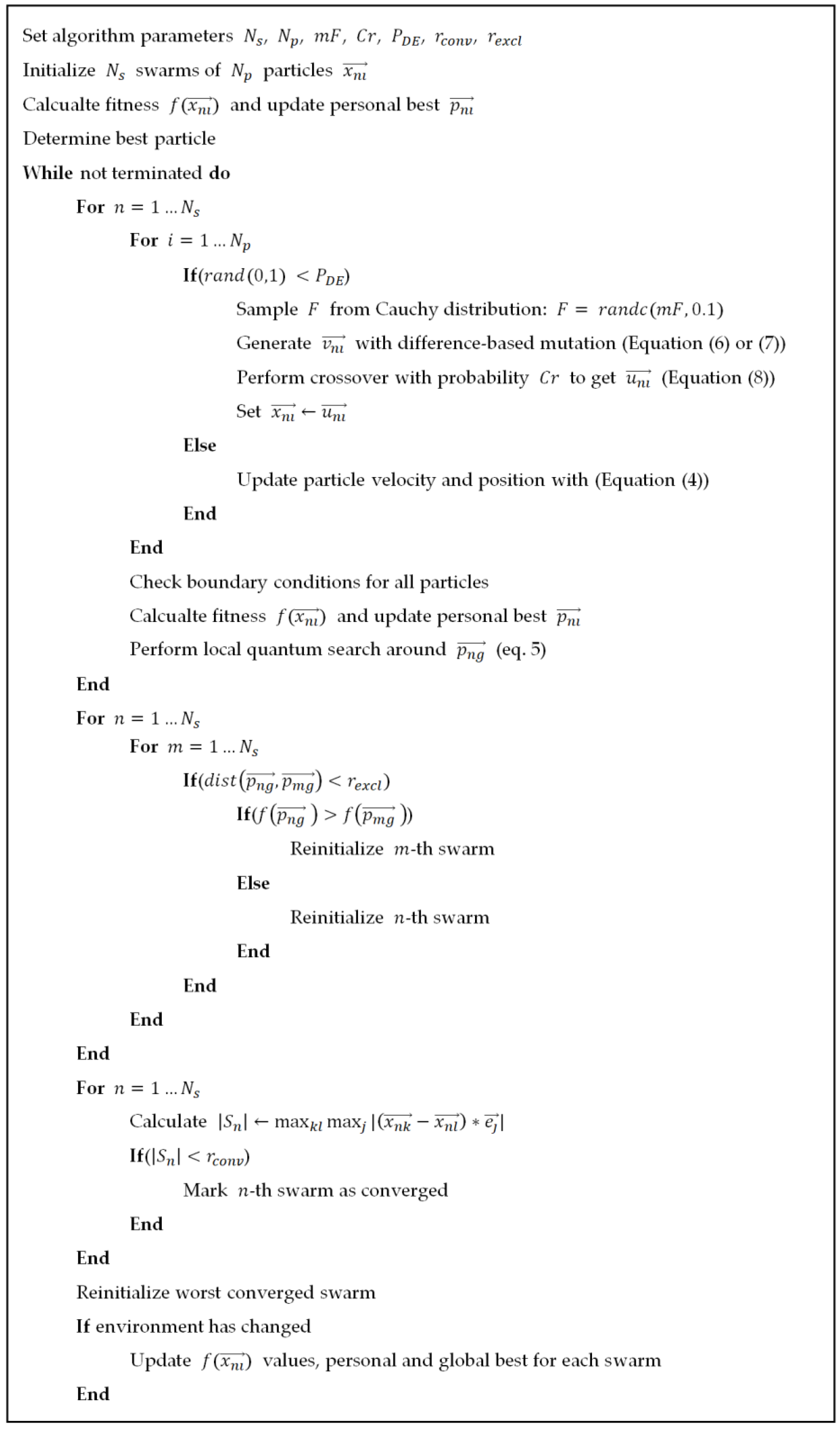
The pseudocode of the proposed mQSODE algorithm is shown in Figure 1.

3. Results

3.1. Experimental Setup

The experiments in this study are performed on the GMPB test suite, the parameters are set equal to those in [10] and given in Table 1.
There settings considered in this study were: a standard computational resource of 5000 function evaluations between changes, decreased to 2500 function evaluations; with the number of peaks increased to 25, and shift severities increased from 2 to 4. The settings are provided in Table 2.
The following algorithms parameters were set for both mQSO and mQSODE algorithms:
  • Number of swarms N s = 10 (independent of the number of components),
  • Number of quantum points N q = 5 ,
  • w = 0.7298 , c 1 = 2.05 and c 2 = 2.05 ,
  • r c l o u d = 2 , r c o n v = r e x c l = 0.5 ( U b L b ) / N s d
  • Number of algorithm runs: 31.
The number of individuals in each swarm N p , probability of applying differential mutation and binomial crossover P D E , type of mutation operator, m F and C r were varied in the experiments:
  • N p = { 5 , 9 , 13 , 17 , 21 , 25 , 29 , 33 }
  • P D E = { 0.1 , 0.2 , 0.3 }
  • Type of mutation: based on current points and based on personal best
  • m F = { 0.1 , 0.2 , 0.3 , 0.4 , 0.5 , 0.6 , 0.7 , 0.8 , 0.9 , 1 }
  • C r = { 0.1 , 0.2 , 0.3 , 0.4 , 0.5 , 0.6 , 0.7 , 0.8 , 0.9 , 1 }
The tested variants further in the text are marked as mQSO N p , mQSODE N p , P D E , x m F , C r for mutation based on current positions, and mQSODE N p , P D E , p m F , C r for mutation based on personal best positions. If the upper indexes for mQSODE are missing, e.g., mQSODE N p , P D E , x , then m F = 0.3 , C r = 1 .
There were two performance indicators used in this study: E B C C , and E O . The E B C C is calculated as follows:
E B C C = 1 T v ˜ t = 1 T φ = 1 v ˜ ( f ( t ) ( x ( t ) ) f ( t ) ( x * ( t ) ) ) ,
where x ( t ) is the optimum position at time t, and x * ( t ) is the best-found position. The offline error E O is calculated as the average error of the best-found position over all fitness evaluations:
E O = 1 T v ˜ t = 1 T φ = 1 v ˜ ( f ( t ) ( x ( t ) ) f ( t ) ( x * ( t 1 ) v ˜ + φ ) )
In the next subsection, the results of sensitivity analysis to the mentioned parameters are provided.

3.2. Results of Computational Experiments

In the first series of experiments, the influence of the population size on the performance of the mQSO algorithm is determined. In Table 3 the mean and standard deviations of the performance indicators are shown. The best results in Table 3, Table 4, Table 5, Table 6, Table 7, Table 8 and Table 9 are highlighted in bold case.
As can be seen from Table 3, the GMPB test suite seems to favor larger population sizes, i.e., the best results were achieved with more than 20 individuals in each of the swarms. The reason for this could be that, unlike MPB, GMPB generates more complex terrains of the goal function after every change, and larger populations with increased diversity are able to locate better local optima. The best results were achieved by mQSO 29 .
In Table 4, the mQSODE algorithm is tested with P D E = 0.1 and two different types of mutation: using current and personal best positions of each particle.
The obtained results shown in Table 4 demonstrate that using the personal best positions of each particle instead of the current position allows for achieving significantly better results across different population sizes. The reason for such behavior could be that the current positions of particles are changing with every iteration, while personal best positions are rather fixed and contain some important information about the problem at hand, such as the location of local optima. Utilizing this information with differential search operators promotes exploration and moving particles in more preferable directions. The best results were achieved by mQSODE 21 , 0.1 , p .
Table 5 contains the comparison of mQSODE with increased P D E probabilities, the personal best positions are used in mutation.
The results in Table 5 show that increasing the probability of using the DE search operator decreases the performance of mQSODE, and P D E = 0.3 is worse than P D E = 0.2 and, compared to Table 4, P D E = 0.2 is worse than P D E = 0.1 . This means that switching the main search mechanism to DE is not desirable for dynamic environments, and the application of DE should be assisting PSO, but not replacing it. It is also important to mention that the best results for the case of P D E = 0.2 were achieved with a smaller number of particles than with P D E = 0.1 , which means that more often applications of DE increase the diversity of individual swarms so that smaller swarm sizes are sufficient.
The sensitivity of mQSODE to crossover rates and scaling factor values were tested and obtained results are demonstrated in Table 6 and Table 7.
The comparison of performance metric values in Table 6 and Table 7 shows that DE search parameters do not have a significant influence on the final performance, however, the influence of scaling factor sampling parameter m F is larger than the influence of crossover rate C r . The best performing configuration here is mQSODE 21 , 0.1 , p 0.3 , 1.0 .
Table 8 contains the comparison of two tested algorithms in this study, mQSO 29 and mQSODE 21 , 0.1 , p with alternative approaches on the same benchmark.
Table 8 shows that although the mQSODE 21 , 0.1 , p is not capable of outperforming some of the alternative methods, it is still highly efficient compared to PSO-based algorithms, such as FTmPSO and mPSO. In particular, it achieves better results in terms of offline error E O especially for more challenging settings 3 and 4. It should be noted that unlike the algorithms from [10], in this study the shift severity learning was not performed, and the shift severity value was set to 2, which is used by quantum particles.
Table 9 contains the results of pairwise Mann-Whitney statistical tests applied to mQSO with two population sizes and mQSODE. The statistical tests were performed with a significance level p = 0.01 , with normal approximation and tie-breaking. The values in Table 3 are the test result (Z-score), where the test result is either -1 (worse), 0 (equal), or 1 (better). For example, if the absolute value of Z was smaller than 2.58, the test result was 0.
With the same population size, the mQSODE algorithms were able to significantly outperform the mQSO in the third setting, i.e., when the number of components is increased to 25. Comparing with mQSO 29 , the mQSODE 21 , 0.1 , p always performs better, except for the fourth setting, although these improvements are not significant according to the Mann-Whitney test.
Figure 2 shows the current error graphs of mQSO 29 and mQSODE 21 , 0.1 , p algorithms for four considered settings, and Figure 3 shows the offline error graphs.
Analyzing Figure 2 and Figure 3 it can be noted that mQSODE 21 , 0.1 , p is more conservative at the beginning, i.e., during the first several environmental changes, while mQSO 29 achieves better values. However, at the final environmental changes both current and offline errors of the modified algorithm are better, which indicates that it makes a better job tracking the local optima. To analyze the reasons for increased performance in the long term, the diversity measure was used for three algorithms, namely mQSO 21 , mQSO 29 , and mQSODE 21 , 0.1 , p . The diversity was measured at every iteration as follows:
D M = 1 N s i = 1 N p j = i N p k = 1 D ( x n i k x n j k ) 2
In other words, the D M was calculated as the sum of pairwise distances between all particles in each swarm and averaged over the number of swarms. Figure 4 shows the diversity measures for one of the runs with setting 1 of the three mentioned algorithms.
The graphs in Figure 4 show that given the same population size, the algorithm without a DE search operator has significantly smaller diversity, up to several times smaller. When comparing mQSODE 21 , 0.1 , p with mQSO 29 , which has a larger population, the diversity of the mQSO after an environmental change is usually larger, however, before the change when the swarms are converged, the diversity measures of these algorithms are comparable, which explains their similar performance.
To compare the efficiency of all the tested modifications, the ranking procedure from the Friedman statistical test was applied, which will further be referred to as the Friedman ranking. To perform such a comparison, all algorithms’ results over 31 independent runs were ranked for every benchmark setting and every performance measure. After this, the ranks assigned to each algorithm participating in the comparison were summed together to form a single rank, which is depicted as a bar in a bar plot in Figure 5. Such a procedure allows for aggregating different performance measures and test scenarios in a single measure, highlighting the best approaches.
The presented Friedman ranking in Figure 5 shows that the mQSODE 21 , 0.1 , p is the best algorithm among the tested configurations. It also shows that applying larger P D E values are inefficient, as well as using current particles’ positions for differential mutation.

4. Discussion

The performed computational experiments and sensitivity analysis have shown that it is possible to develop an efficient hybrid approach, combining PSO and DE. The key to efficient performance here seems to be in the usage of personal best positions of particles instead of current positions because personal best points contain important information for the search process.
Although within this study only one baseline algorithm was considered, namely mQSO, it is possible to interpolate the proposed algorithmic scheme for any other PSO-based algorithm, and most of the used approaches for dynamic optimization are based on a type of swarm intelligence algorithm derived from particle swarm optimization. Thus, the findings of this study could be considered rather general; however, additional experiments in other scenarios are required to prove the concept.
It is rather obvious that setting the probability of applying DE to a fixed value during the whole algorithm run is not the best possible option, and a specific adaptation mechanism for P D E should be developed. In our preliminary experiments with several adaptation schemes, we were not able to come up with an efficient method that would significantly improve the performance of the GMPB test suite. The reason for that was that DE mutation generates successful solutions more often so allowing the P D E to be adapted simply increases this probability to the upper threshold. This, in turn, results in too high P D E values, which decrease the search efficiency, as was shown in the experiments in this study. In other words, the adaptation scheme should consider this fact and be less greedy for improvements.
In addition to P D E adaptation, application of DE operators burdens researchers with additional parameters to be tuned, namely the scaling factor F and crossover rate C r . In this study, it was shown that the sensitivity to these values is not very large, probably thanks to the rotation-invariant nature of PSO and applied sampling of F values from the Cauchy distribution. Nevertheless, incorporating known adaptation schemes, such as success-history adaptation, or developing new specific methods is another direction of further studies.
Finally, it should be mentioned that in this study only one differential mutation strategy was tested, i.e., the classical rand/1, although other schemes are known to be superior in certain cases. If some of them would be shown to perform better than rand/1 for dynamic environments, this will allow making another step in the direction toward efficient DOPs solvers.

5. Conclusions

In this study, the modification of the Quantum Multi-Swarm Optimization algorithm was proposed. The algorithm incorporating the additional search operator from Differential Evolution, mQSODE, has shown to perform better in different challenging settings of the generalized moving peaks benchmark. Thus, in this study, it was shown that although the DE algorithms usually show worse results in dynamically changing environments, the exploration capabilities of their mutation operator can be efficiently used to modify the existing algorithms if they are applied to personal best positions of the points in PSO. Further research directions may include applying other differential search operators to mQSO, developing adaptation schemes, or modifying other algorithms in a similar manner.

Author Contributions

Conceptualization, V.S., S.A. and A.V.; methodology, V.S., S.A., A.V. and E.S. (Evgenii Sopov); software, V.S. and S.A.; validation, A.V., S.A. and E.S. (Eugene Semenkin); formal analysis, E.S. (Evgenii Sopov) and M.A.; investigation, S.A. and A.V.; resources, V.S. and E.S. (Evgenii Sopov); data curation, S.A. and A.V.; writing—original draft preparation, V.S., S.A. and A.V.; writing—review and editing, E.S. (Evgenii Sopov), E.S. (Eugene Semenkin) and M.A.; visualization, V.S.; supervision, E.S. (Eugene Semenkin) and M.A.; project administration, E.S. (Evgenii Sopov) and E.S. (Eugene Semenkin); funding acquisition, E.S. (Eugene Semenkin) and M.A. All authors have read and agreed to the published version of the manuscript.

Funding

The reported study was funded by RFBR and FWF according to the research project №21-51-14003.

Data Availability Statement

Not applicable.

Conflicts of Interest

The authors declare no conflict of interest.

References

  1. Yar, M.H.; Rahmati, V.; Oskouei, H.R.D. A Survey on Evolutionary Computation: Methods and Their Applications in Engineerng. Mod. Appl. Sci. 2016, 10, 131–139. [Google Scholar] [CrossRef] [Green Version]
  2. Nguyen, T.T.; Yang, S.; Branke, J. Evolutionary dynamic optimization: A survey of the state of the art. Swarm Evol. Comput. 2012, 6, 1–24. [Google Scholar] [CrossRef]
  3. Yazdani, D.; Cheng, R.; Yazdani, D.; Branke, J.; Jin, Y.; Yao, X. A Survey of Evolutionary Continuous Dynamic Optimization Over Two Decades—Part A. IEEE Trans. Evol. Comput. 2021, 25, 609–629. [Google Scholar] [CrossRef]
  4. Yazdani, D.; Cheng, R.; Yazdani, D.; Branke, J.; Jin, Y.; Yao, X. A Survey of Evolutionary Continuous Dynamic Optimization Over Two Decades—Part B. IEEE Trans. Evol. Comput. 2021, 25, 630–650. [Google Scholar] [CrossRef]
  5. Elshamli, A.; Abdullah, H.A.; Areibi, S. Genetic algorithm for dynamic path planning. Can. Conf. Electr. Comput. Eng. 2004, 2, 677–680. [Google Scholar]
  6. Michalewicz, Z.; Schmidt, M.; Michalewicz, M.; Chiriac, C. Adaptive business intelligence: Three case studies. Stud. Comput. Intell. 2007, 51, 179–196. [Google Scholar]
  7. Kyriakakis, N.A.; Marinaki, M.; Matsatsinis, N.F.; Marinakis, Y. Moving peak drone search problem: An online multi-swarm intelligence approach for UAV search operations. Swarm Evol. Comput. 2021, 66, 100956. [Google Scholar] [CrossRef]
  8. Branke, J. Memory enhanced evolutionary algorithms for changing optimization problems. In Proceedings of the 1999 Congress on Evolutionary Computation-CEC99, Washington, DC, USA, 6–9 July 1999; Volume 3, pp. 1875–1882. [Google Scholar]
  9. Li, C.; Yang, S. A generalized approach to construct benchmark problems for dynamic optimization, in Simulated Evolution and Learning. In Lecture Notes in Computer Science; Springer: Berlin/Heidelberg, Germany, 2013; Volume 5361, pp. 391–400. [Google Scholar]
  10. Yazdani, B.D.; Omidvar, M.N.; Cheng, R.; Branke, J.; Nguyen, T.; Yao, X. Benchmarking Continuous Dynamic Optimization: Survey and Generalized Test Suite. IEEE Trans. Cybern. 2020, 1, 1–14. [Google Scholar] [CrossRef]
  11. Yazdani, D.; Branke, J.; Omidvar, M.N.; Li, X.; Li, C.; Mavrovouniotis, M.; Nguyen, T.T.; Yang, S.; Yao, X. IEEE CEC 2022 Competition on Dynamic Optimization Problems Generated by Generalized Moving Peaks Benchmark; Technical Report; Southern University of Science and Technology: Shenzhen, China, 2021. [Google Scholar]
  12. Ahrari, A.; Elsayed, S.M.; Sarker, R.A.; Essam, D.L.; Coello, C.A. A Novel Parametric benchmark generator for dynamic multimodal optimization. Swarm Evol. Comput. 2021, 65, 100924. [Google Scholar] [CrossRef]
  13. Blackwell, T.M.; Branke, J. Multiswarms, exclusion, and anti-convergence in dynamic environments. IEEE Trans. Evol. Comput. 2006, 10, 459–472. [Google Scholar] [CrossRef]
  14. Yazdani, D.; Nasiri, B.; Sepas-Moghaddam, A.; Meybodi, M.R. A novel multi-swarm algorithm for optimization in dynamic environments based on particle swarm optimization. Appl. Soft Comput. 2013, 13, 2144–2158. [Google Scholar] [CrossRef]
  15. Plessis, M.C.; Engelbrecht, A.P. Differential evolution for dynamic environments with unknown numbers of optima. J. Glob. Optim. 2013, 55, 73–99. [Google Scholar] [CrossRef] [Green Version]
  16. Jia, D. A Culture-Based Artificial Bee Colony Algorithm for Optimization in Dynamic Environments. J. Adv. Comput. Intell. Intell. Inform. 2022, 26, 23–27. [Google Scholar] [CrossRef]
  17. Hu, X.; Eberhart, R. Adaptive particle swarm optimisation: Detection and response to dynamic systems. In Proceedings of the IEEE Congress on Evolutionary Computation, Honolulu, HI, USA, 12–17 May 2002; pp. 1666–1670. [Google Scholar]
  18. Cobb, H.G. An Investigation into the Use of Hypermutation as an Adaptive Operator in Genetic Algorithms Having Continuous, Time-Dependent Nonstationary Environments; Technical Report AIC-90-001; Naval Research Lab: Washington, DC, USA, 1990. [Google Scholar]
  19. Riekert, M.; Malan, K.M.; Engelbrecht, A.P. Adaptive genetic programming for dynamic classification problems. In Proceedings of the IEEE Congress on Evolutionary Computation, Trondheim, Norway, 18–21 May 2009; pp. 674–681. [Google Scholar]
  20. Grefenstette, J.J. Genetic algorithms for changing environments. Parallel Probl. Solving Nat. 1992, 2, 137–144. [Google Scholar]
  21. Morrison, R.W. Designing Evolutionary Algorithms for Dynamic Environments; Springer: Berlin/Heidelberg, Germany, 2004. [Google Scholar]
  22. Daneshyari, M.; Yen, G. Dynamic optimization using cultural based PSO. In Proceedings of the IEEE Congress on Evolutionary Computation, New Orleans, LA, USA, 5–8 June 2011; pp. 509–516. [Google Scholar]
  23. Simoes, A.; Costa, E. Memory-based CHC algorithms for the dynamic—Traveling salesman problem. In Proceedings of the Genetic and Evolutionary Computation Conference, New York, NY, USA, 12–16 July 2011; pp. 1037–1044. [Google Scholar]
  24. Hatzakis, I.; Wallace, D. Dynamic multi-objective optimization with evolutionary algorithms: A forward-looking approach. In Proceedings of the Genetic and Evolutionary Computation Conference, New York, NY, USA, 8–12 July 2006; pp. 1201–1208. [Google Scholar]
  25. Oppacher, F.; Wineberg, M. The shifting balance genetic algorithm: Improving the GA in a dynamic environment. In Proceedings of the Genetic and Evolutionary Computation Conference, San Francisco, CA, USA, 13–17 July 1999; Volume 1, pp. 504–510. [Google Scholar]
  26. Ursem, R.K. Multinational GA optimization techniques in dynamic environments. In Proceedings of the Genetic and Evolutionary Computation Conference, San Francisco, CA, USA, 10–12 July 2000; pp. 19–26. [Google Scholar]
  27. Qin, J.; Huang, C.; Luo, Y. Adaptive multi-swarm in dynamic environments. Swarm Evol. Comput. 2021, 63, 100870. [Google Scholar] [CrossRef]
  28. Li, C.; Nguyen, T.; Yang, M.; Mavrovouniotis, M.; Yang, S. An Adaptive Multipopulation Framework for Locating and Tracking Multiple Optima. IEEE Trans. Evol. Comput. 2016, 20, 590–605. [Google Scholar] [CrossRef] [Green Version]
  29. Tao, X.; Guo, W.; Li, X.; He, Q.; Liu, R.; Zou, J. Fitness peak clustering based dynamic multi-swarm particle swarm optimization with enhanced learning strategy. Expert Syst. Appl. 2022, 191, 116301. [Google Scholar] [CrossRef]
  30. Li, C.; Yang, S.; Yang, M. An Adaptive Multi-Swarm Optimizer for Dynamic Optimization Problems. Evol. Comput. 2014, 22, 559–594. [Google Scholar] [CrossRef]
  31. Xia, X.; Tang, Y.; Wei, B.; Zhang, Y.; Gui, L.; Li, X. Dynamic multi-swarm global particle swarm optimization. Computing 2020, 102, 1587–1626. [Google Scholar] [CrossRef]
  32. Xia, X.; Tang, Y.; Wei, B.; Gui, L. Dynamic Multi-Swarm Particle Swarm Optimization Based on Elite Learning. IEEE Access 2019, 7, 184849–184865. [Google Scholar] [CrossRef]
  33. Awad, N.H.; Ali, M.Z.; Liang, J.J.; Qu, B.Y.; Suganthan, P.N. Problem Definitions and Evaluation Criteria for the CEC 2017 Special Session and Competition on Single Objective Real-Parameter Numerical Operation; Technical Report; Nanyang Technological University: Singapore, 2016. [Google Scholar]
  34. Song, L.; Shi, J.; Pan, A.; Yang, J.; Xie, J. A Dynamic Multi-Swarm Particle Swarm Optimizer for Multi-Objective Optimization of Machining Operations Considering Efficiency and Energy Consumption. Energies 2020, 13, 2616. [Google Scholar] [CrossRef]
  35. Zhao, Q.; Li, C. Two-Stage Multi-Swarm Particle Swarm Optimizer for Unconstrained and Constrained Global Optimization. IEEE Access 2020, 8, 124905–124927. [Google Scholar] [CrossRef]
  36. Sedki, A.; Ouazar, D. Hybrid particle swarm optimization and differential evolution for optimal design of water distribution systems. Adv. Eng. Inform. 2012, 26, 582–591. [Google Scholar] [CrossRef]
  37. Lynn, N.; Ali, M.; Suganthan, P.N. Population topologies for particle swarm optimization and differential evolution. Swarm Evol. Comput. 2018, 39, 24–35. [Google Scholar] [CrossRef]
  38. Akhmedova, S.; Stanovov, V.; Semenkin, E. Soft island model for population-based optimization algorithms. In International Conference on Swarm Intelligence; Springer: Cham, Switzerland, 2018; pp. 68–77. [Google Scholar]
  39. Zhang, J.; Sanderson, A.C. JADE: Self-adaptive differential evolution with fast and reliable convergence performance. In Proceedings of the IEEE Congress on Evolutionary Computation, Singapore, 25–28 September 2007; pp. 2251–2258. [Google Scholar]
Figure 1. Pseudocode of the proposed mQSODE algorithm.
Algorithms 15 00154 g001
Figure 2. Current error graphs of mQSO 29 and mQSODE 21 , 0.1 , p in four benchmark settings.
Algorithms 15 00154 g002
Figure 3. Offline error graphs of three tested algorithms with two benchmark cases: 2000 and 5000 function evaluations between changes.
Algorithms 15 00154 g003
Figure 4. Diversity measures of mQSO 21 , mQSO 29 and mQSODE 21 , 0.1 , p , setting 1.
Algorithms 15 00154 g004
Figure 5. Bar plot Friedman ranks of tested algorithms, aggregated over four settings.
Algorithms 15 00154 g005
Table 1. The set of Generalized Moving Peaks Benchmark (GMPB) parameters.
ParameterSymbolValue
Dimensiond10
Shift severity s ˜ 2, 4
Number of componentsm10, 25
Angle severity θ ˜ π / 9
Height severity h ˜ 7
Width severity w ˜ 1
Irregularity   parameter   τ severity τ ˜ 0.05
Irregularity   parameter   η severity η ˜ 2
Search range [ L b , U b ] d [ 50 , 50 ] d
Height range [ h m i n , h m a x ] [ 30 , 70 ]
Width range [ w m i n , w m a x ] d [ 1 , 12 ] d
Angle range [ θ m i n , θ m a x ] [ π , π ]
Irregularity   parameter   τ range [ τ m i n , τ m a x ] [ 0 , 0.4 ]
Irregularity   parameter   η range [ η m i n , η m a x ] [ 10 , 25 ]
Initial center position c k ( 0 ) U [ L b , U b ] d
Initial height h k ( 0 ) U [ h m i n , h m a x ]
Initial width w k ( 0 ) U [ w m i n , w m a x ] d
Initial angle θ k ( 0 ) U [ θ m i n , θ m a x ]
Initial   irregularity   parameter   τ τ k ( 0 ) U [ τ m i n , τ m a x ]
Initial   irregularity   parameter   η η k ( 0 ) U [ η m i n , η m a x ] d
Initial rotation matrix R k ( 0 ) G S ( N o r m ( 0 , 1 ) d × d )
Change frequency v ˜ 2500, 5000
Number of EnvironmentsT100
Table 2. Tested settings.
ParameterSymbolSetting 1Setting 2Setting 3Setting 4
Shift severities s ˜ 2422
Numbers of componentsm10102510
Change frequency v ˜ 5000500050002500
Table 3. Comparison of mQSO with different population sizes.
AlgorithmSetting 1Setting 2
E B B C E O E B B C E O
mQSO 5 25.53 ± 5.54 29.72 ± 5.94 32.67 ± 5.39 39.09 ± 5.67
mQSO 9 14.29 ± 3.07 18.05 ± 3.18 17.97 ± 3.53 24.11 ± 3.60
mQSO 13 11.71 ± 1.89 15.47 ± 1.98 15.22 ± 2.67 21.27 ± 2.80
mQSO 17 10.16 ± 1.81 14.03 ± 1.94 13.30 ± 2.25 19.38 ± 2.46
mQSO 21 9.40 ± 2.21 13.18 ± 2.21 12.60 ± 1.52 18.60 ± 1.71
mQSO 25 9.12 ± 1.58 13.13 ± 1.77 12.31 ± 1.60 18.47 ± 1.75
mQSO 29 9.00 ± 1.64 12.99 ± 1.76 12.66 ± 1.90 18.85 ± 2.19
mQSO 33 8.70 ± 1.29 12.76 ± 1.43 12.55 ± 1.50 18.86 ± 1.68
AlgorithmSetting 3Setting 4
E B B C E O E B B C E O
mQSO 5 24.36 ± 3.40 28.09 ± 3.68 27.21 ± 5.82 31.86 ± 6.23
mQSO 9 14.22 ± 1.97 17.68 ± 2.08 16.96 ± 2.84 21.34 ± 2.99
mQSO 13 11.83 ± 1.34 15.31 ± 1.41 14.42 ± 2.18 18.83 ± 2.36
mQSO 17 10.43 ± 1.21 13.95 ± 1.26 13.71 ± 2.06 18.39 ± 2.43
mQSO 21 10.06 ± 1.28 13.54 ± 1.35 13.65 ± 2.00 18.33 ± 2.33
mQSO 25 9.57 ± 1.17 13.19 ± 1.24 13.34 ± 1.63 18.08 ± 2.17
mQSO 29 9.26 ± 1.13 12.89 ± 1.29 13.20 ± 1.45 18.41 ± 2.06
mQSO 33 9.38 ± 1.02 13.14 ± 1.11 14.11 ± 1.55 19.11 ± 1.86
Table 4. Comparison of mQSODE with current and personal best positions in mutation.
AlgorithmSetting 1Setting 2
E B B C E O E B B C E O
mQSODE 5 , 0.1 , x 17.66 ± 3.05 21.34 ± 3.29 22.46 ± 2.02 27.97 ± 1.96
mQSODE 9 , 0.1 , x 12.47 ± 1.95 15.91 ± 2.14 17.90 ± 2.64 23.20 ± 2.72
mQSODE 13 , 0.1 , x 12.32 ± 2.01 15.74 ± 1.97 17.75 ± 1.86 22.92 ± 2.03
mQSODE 17 , 0.1 , x 12.43 ± 1.61 15.77 ± 1.81 18.05 ± 1.80 23.31 ± 1.93
mQSODE 21 , 0.1 , x 12.87 ± 1.62 16.41 ± 1.85 18.31 ± 1.93 23.57 ± 2.14
mQSODE 25 , 0.1 , x 13.00 ± 1.41 16.48 ± 1.64 18.35 ± 1.73 23.68 ± 2.01
mQSODE 29 , 0.1 , x 13.16 ± 1.45 16.72 ± 1.63 18.52 ± 1.76 23.86 ± 1.91
mQSODE 33 , 0.1 , x 13.31 ± 1.44 16.80 ± 1.68 19.09 ± 1.43 24.35 ± 1.52
mQSODE 5 , 0.1 , p 18.56 ± 3.49 22.48 ± 3.75 24.40 ± 4.04 30.58 ± 4.17
mQSODE 9 , 0.1 , p 10.72 ± 2.50 14.35 ± 2.68 14.49 ± 2.19 20.29 ± 2.17
mQSODE 13 , 0.1 , p 9.23 ± 1.77 12.91 ± 1.85 12.87 ± 2.05 18.56 ± 2.23
mQSODE 17 , 0.1 , p 8.61 ± 1.13 12.05 ± 1.19 12.58 ± 1.41 18.14 ± 1.65
mQSODE 21 , 0.1 , p 8.50 ± 1.26 12.18 ± 1.39 12.35 ± 1.21 18.05 ± 1.28
mQSODE 25 , 0.1 , p 8.52 ± 0.95 12.25 ± 1.03 12.85 ± 1.14 18.46 ± 1.35
mQSODE 29 , 0.1 , p 8.41 ± 0.90 12.19 ± 1.03 13.13 ± 0.97 18.80 ± 1.11
mQSODE 33 , 0.1 , p 8.84 ± 1.05 12.60 ± 1.13 13.19 ± 0.91 18.82 ± 1.14
AlgorithmSetting 3Setting 4
E B B C E O E B B C E O
mQSODE 5 , 0.1 , x 17.97 ± 2.45 21.41 ± 2.62 23.33 ± 4.21 27.77 ± 4.60
mQSODE 9 , 0.1 , x 13.48 ± 1.99 16.75 ± 2.11 18.73 ± 2.60 22.81 ± 2.68
mQSODE 13 , 0.1 , x 13.08 ± 1.57 16.17 ± 1.67 18.55 ± 2.61 22.74 ± 2.84
mQSODE 17 , 0.1 , x 13.58 ± 1.51 16.81 ± 1.58 19.00 ± 2.23 23.21 ± 2.65
mQSODE 21 , 0.1 , x 13.91 ± 1.83 17.16 ± 2.07 18.78 ± 2.14 22.94 ± 2.22
mQSODE 25 , 0.1 , x 13.94 ± 1.47 17.22 ± 1.56 19.33 ± 2.01 23.80 ± 2.55
mQSODE 29 , 0.1 , x 14.47 ± 1.52 17.82 ± 1.59 20.12 ± 2.14 24.84 ± 2.54
mQSODE 33 , 0.1 , x 14.30 ± 1.28 17.58 ± 1.41 20.60 ± 2.03 25.34 ± 2.30
mQSODE 5 , 0.1 , p 17.96 ± 2.16 21.54 ± 2.17 22.16 ± 4.74 26.66 ± 5.08
mQSODE 9 , 0.1 , p 11.24 ± 1.70 14.59 ± 1.71 15.39 ± 2.26 19.81 ± 2.48
mQSODE 13 , 0.1 , p 9.61 ± 1.32 12.97 ± 1.35 13.60 ± 2.41 17.68 ± 2.68
mQSODE 17 , 0.1 , p 9.50 ± 1.36 13.00 ± 1.46 13.19 ± 1.65 17.68 ± 1.88
mQSODE 21 , 0.1 , p 9.09 ± 1.06 12.48 ± 1.10 13.48 ± 1.39 17.75 ± 1.65
mQSODE 25 , 0.1 , p 9.65 ± 1.10 13.05 ± 1.18 14.19 ± 1.38 18.73 ± 1.94
mQSODE 29 , 0.1 , p 9.66 ± 0.88 13.06 ± 0.94 14.73 ± 1.76 19.73 ± 2.27
mQSODE 33 , 0.1 , p 10.05 ± 0.91 13.49 ± 0.99 15.39 ± 1.69 19.97 ± 2.11
Table 5. Comparison of mQSODE, with P D E = 0.2 and P D E = 0.3 .
AlgorithmSetting 1Setting 2
E B B C E O E B B C E O
mQSODE 5 , 0.2 , p 18.16 ± 2.4322.01 ± 2.6123.83 ± 3.2530.06 ± 3.42
mQSODE 9 , 0.2 , p 10.41 ± 1.8114.15 ± 2.1014.23 ± 1.7120.02 ± 1.72
mQSODE 13 , 0.2 , p 8.75 ± 1.0812.25 ± 1.2113.06 ± 1.3318.72 ± 1.43
mQSODE 17 , 0.2 , p 8.82 ± 1.7912.41 ± 1.9113.01 ± 1.4318.57 ± 1.53
mQSODE 21 , 0.2 , p 9.13 ± 1.3712.80 ± 1.5213.23 ± 1.2518.82 ± 1.53
mQSODE 25 , 0.2 , p 8.82 ± 0.8212.35 ± 1.0613.85 ± 1.3519.35 ± 1.57
mQSODE 29 , 0.2 , p 9.36 ± 1.1212.93 ± 1.2914.09 ± 1.2719.42 ± 1.45
mQSODE 33 , 0.2 , p 9.81 ± 1.3613.49 ± 1.4614.57 ± 0.9719.99 ± 1.17
mQSODE 5 , 0.3 , p 19.80 ± 3.9424.01 ± 4.4025.93 ± 4.1632.53 ± 4.37
mQSODE 9 , 0.3 , p 10.78 ± 1.7314.68 ± 1.8415.31 ± 2.5121.45 ± 2.70
mQSODE 13 , 0.3 , p 9.51 ± 1.5013.14 ± 1.7013.62 ± 1.6319.48 ± 1.74
mQSODE 17 , 0.3 , p 8.97 ± 1.1712.56 ± 1.3113.83 ± 1.2619.57 ± 1.45
mQSODE 21 , 0.3 , p 9.25 ± 1.3812.89 ± 1.5414.05 ± 1.4619.62 ± 1.72
mQSODE 25 , 0.3 , p 9.45 ± 0.9713.13 ± 1.2314.38 ± 1.0319.91 ± 1.16
mQSODE 29 , 0.3 , p 9.66 ± 0.9313.31 ± 1.0914.95 ± 1.0920.29 ± 1.19
mQSODE 33 , 0.3 , p 10.34 ± 1.1713.93 ± 1.3015.25 ± 1.4420.88 ± 1.71
AlgorithmSetting 3Setting 4
E B B C E O E B B C E O
mQSODE 5 , 0.2 , p 18.76 ± 2.6422.54 ± 2.7421.69 ± 3.1226.17 ± 3.25
mQSODE 9 , 0.2 , p 10.95 ± 1.4014.44 ± 1.4214.40 ± 1.7218.90 ± 2.16
mQSODE 13 , 0.2 , p 9.76 ± 1.4813.16 ± 1.5414.10 ± 2.3118.53 ± 2.57
mQSODE 17 , 0.2 , p 9.97 ± 1.1113.32 ± 1.0914.76 ± 1.4118.97 ± 1.49
mQSODE 21 , 0.2 , p 9.91 ± 0.9713.22 ± 1.0514.67 ± 2.0718.98 ± 2.25
mQSODE 25 , 0.2 , p 9.97 ± 0.8913.25 ± 1.0115.17 ± 1.6319.44 ± 2.00
mQSODE 29 , 0.2 , p 10.61 ± 0.9213.89 ± 1.0315.85 ± 1.7120.18 ± 2.02
mQSODE 33 , 0.2 , p 11.06 ± 0.9814.36 ± 1.0817.16 ± 1.9621.90 ± 2.36
mQSODE 5 , 0.3 , p 19.00 ± 2.9522.79 ± 3.2323.22 ± 2.8227.98 ± 3.14
mQSODE 9 , 0.3 , p 11.92 ± 1.8215.47 ± 1.8816.19 ± 2.5420.56 ± 2.61
mQSODE 13 , 0.3 , p 10.29 ± 1.3513.69 ± 1.3814.91 ± 2.0418.98 ± 2.34
mQSODE 17 , 0.3 , p 10.33 ± 1.1713.75 ± 1.2814.67 ± 1.3719.01 ± 1.53
mQSODE 21 , 0.3 , p 10.16 ± 1.1613.50 ± 1.2915.09 ± 1.5619.44 ± 1.96
mQSODE 25 , 0.3 , p 10.87 ± 0.8814.21 ± 1.0115.96 ± 1.3720.33 ± 1.52
mQSODE 29 , 0.3 , p 11.02 ± 0.7314.35 ± 0.9016.95 ± 1.7021.15 ± 1.99
mQSODE 33 , 0.3 , p 11.53 ± 0.9214.84 ± 1.0617.45 ± 1.6721.81 ± 2.02
Table 6. Comparison of mQSODE with different crossover rates.
AlgorithmSetting 1Setting 2
E B B C E O E B B C E O
mQSODE 21 , 0.1 , p 0.3 , 0.1 8.70 ± 1.70 12.38 ± 1.79 12.39 ± 1.52 17.95 ± 1.66
mQSODE 21 , 0.1 , p 0.3 , 0.2 8.35 ± 1.26 12.00 ± 1.36 12.41 ± 1.38 18.05 ± 1.69
mQSODE 21 , 0.1 , p 0.3 , 0.3 8.29 ± 1.40 11.94 ± 1.44 12.38 ± 1.24 18.06 ± 1.47
mQSODE 21 , 0.1 , p 0.3 , 0.4 8.63 ± 1.77 12.26 ± 1.89 12.37 ± 1.42 18.02 ± 1.48
mQSODE 21 , 0.1 , p 0.3 , 0.5 8.49 ± 1.21 12.14 ± 1.25 12.17 ± 1.69 17.71 ± 1.76
mQSODE 21 , 0.1 , p 0.3 , 0.6 8.25 ± 1.10 11.85 ± 1.11 12.06 ± 1.18 17.69 ± 1.35
mQSODE 21 , 0.1 , p 0.3 , 0.7 8.56 ± 1.34 12.24 ± 1.37 12.01 ± 1.24 17.52 ± 1.31
mQSODE 21 , 0.1 , p 0.3 , 0.8 8.46 ± 1.51 12.19 ± 1.56 12.59 ± 1.84 18.25 ± 2.01
mQSODE 21 , 0.1 , p 0.3 , 0.9 8.50 ± 1.11 12.08 ± 1.31 12.59 ± 1.74 18.31 ± 1.87
mQSODE 21 , 0.1 , p 0.3 , 1.0 8.10 ± 0.96 11.80 ± 1.02 12.19 ± 1.24 17.87 ± 1.25
AlgorithmSetting 3Setting 4
E B B C E O E B B C E O
mQSODE 21 , 0.1 , p 0.3 , 0.1 9.11 ± 0.85 12.46 ± 0.83 13.16 ± 1.33 17.66 ± 2.01
mQSODE 21 , 0.1 , p 0.3 , 0.2 9.30 ± 1.08 12.64 ± 1.11 13.17 ± 1.75 17.25 ± 1.98
mQSODE 21 , 0.1 , p 0.3 , 0.3 9.18 ± 0.87 12.51 ± 0.89 13.84 ± 1.53 18.32 ± 2.03
mQSODE 21 , 0.1 , p 0.3 , 0.4 9.28 ± 1.40 12.62 ± 1.49 13.24 ± 1.56 17.67 ± 1.86
mQSODE 21 , 0.1 , p 0.3 , 0.5 8.85 ± 1.14 12.13 ± 1.18 13.55 ± 1.81 17.82 ± 1.87
mQSODE 21 , 0.1 , p 0.3 , 0.6 9.00 ± 1.08 12.43 ± 1.22 13.53 ± 1.36 17.95 ± 1.48
mQSODE 21 , 0.1 , p 0.3 , 0.7 9.50 ± 1.42 12.93 ± 1.54 13.51 ± 1.51 17.69 ± 1.85
mQSODE 21 , 0.1 , p 0.3 , 0.8 9.21 ± 0.95 12.59 ± 1.04 13.57 ± 1.58 18.32 ± 2.14
mQSODE 21 , 0.1 , p 0.3 , 0.9 9.30 ± 1.11 12.65 ± 1.18 13.83 ± 1.31 18.15 ± 1.81
mQSODE 21 , 0.1 , p 0.3 , 1.0 9.12 ± 1.04 12.54 ± 1.12 13.70 ± 1.61 18.21 ± 1.79
Table 7. Comparison of mQSODE, with different scaling factor sampling parameters.
AlgorithmSetting 1Setting 2
E B B C E O E B B C E O
mQSODE 21 , 0.1 , p 0.1 , 1.0 8.09 ± 1.29 11.72 ± 1.38 12.73 ± 1.87 18.43 ± 1.81
mQSODE 21 , 0.1 , p 0.2 , 1.0 8.64 ± 1.45 12.38 ± 1.60 12.28 ± 1.65 17.93 ± 1.80
mQSODE 21 , 0.1 , p 0.3 , 1.0 8.10 ± 0.96 11.80 ± 1.02 12.19 ± 1.24 17.87 ± 1.25
mQSODE 21 , 0.1 , p 0.4 , 1.0 8.23 ± 1.08 11.88 ± 1.16 12.17 ± 1.39 17.70 ± 1.50
mQSODE 21 , 0.1 , p 0.5 , 1.0 8.42 ± 1.24 12.12 ± 1.40 12.63 ± 1.52 18.20 ± 1.77
mQSODE 21 , 0.1 , p 0.6 , 1.0 8.42 ± 1.42 11.87 ± 1.44 12.90 ± 1.30 18.36 ± 1.48
mQSODE 21 , 0.1 , p 0.7 , 1.0 9.00 ± 1.45 12.48 ± 1.50 13.44 ± 1.49 19.04 ± 1.75
mQSODE 21 , 0.1 , p 0.8 , 1.0 9.21 ± 1.33 12.67 ± 1.36 13.34 ± 1.63 18.65 ± 1.71
mQSODE 21 , 0.1 , p 0.9 , 1.0 9.50 ± 1.78 13.23 ± 2.01 13.78 ± 2.02 19.30 ± 2.12
mQSODE 21 , 0.1 , p 1.0 , 1.0 9.02 ± 1.31 12.58 ± 1.35 13.65 ± 1.70 19.13 ± 1.78
AlgorithmSetting 3Setting 4
E B B C E O E B B C E O
mQSODE 21 , 0.1 , p 0.1 , 1.0 9.37 ± 1.30 12.72 ± 1.34 13.29 ± 1.28 17.88 ± 1.74
mQSODE 21 , 0.1 , p 0.2 , 1.0 8.92 ± 0.95 12.30 ± 1.02 13.41 ± 1.74 17.87 ± 2.07
mQSODE 21 , 0.1 , p 0.3 , 1.0 9.12 ± 1.04 12.54 ± 1.12 13.70 ± 1.61 18.21 ± 1.79
mQSODE 21 , 0.1 , p 0.4 , 1.0 9.19 ± 1.01 12.61 ± 1.06 13.65 ± 1.39 18.09 ± 1.60
mQSODE 21 , 0.1 , p 0.5 , 1.0 9.45 ± 1.02 12.82 ± 1.08 14.18 ± 1.68 18.92 ± 2.05
mQSODE 21 , 0.1 , p 0.6 , 1.0 9.65 ± 1.40 12.88 ± 1.36 14.56 ± 1.88 19.03 ± 2.16
mQSODE 21 , 0.1 , p 0.7 , 1.0 9.81 ± 1.37 13.16 ± 1.45 14.79 ± 1.63 19.04 ± 2.04
mQSODE 21 , 0.1 , p 0.8 , 1.0 9.63 ± 1.20 12.87 ± .29 14.92 ± 2.08 19.08 ± 2.34
mQSODE 21 , 0.1 , p 0.9 , 1.0 9.80 ± 1.00 12.98 ± 1.03 14.95 ± 1.69 19.26 ± 1.79
mQSODE 21 , 0.1 , p 1.0 , 1.0 10.34 ± .28 13.62 ± 1.23 14.87 ± 1.53 19.03 ± 1.92
Table 8. Comparison of mQSO and mQSODE with alternative approaches from [10].
AlgorithmSetting 1Setting 2
E B B C E O E B B C E O
mQSO 29 9.00 ± 1.64 12.99 ± 1.76 12.66 ± 1.90 18.85 ± 2.19
mQSODE 21 , 0.1 , p 8.50 ± 1.26 12.18 ± 1.39 12.35 ± 1.21 18.05 ± 1.28
FTmPSO 7.11 ± 0.26 12.70 ± 0.34 8.70 ± 0.26 16.06 ± 0.35
mCMA-ES 5.11 ± 0.22 7.59 ± 0.24 7.39 ± 0.26 11.65 ± 0.28
mPSO 8.51 ± 0.22 12.88 ± 0.27 11.63 ± 0.19 18.52 ± 0.26
AlgorithmSetting 3Setting 4
E B B C E O E B B C E O
mQSO 29 9.26 ± 1.13 12.89 ± 1.29 13.20 ± 1.45 18.41 ± 2.06
mQSODE 21 , 0.1 , p 9.09 ± 1.06 12.48 ± 1.10 13.48 ± 1.39 17.75 ± 1.65
FTmPSO 7.99 ± 0.16 13.48 ± 0.21 11.57 ± 0.32 18.04 ± 0.39
mCMA-ES 6.14 ± 0.15 8.49 ± 0.16 8.56 ± 0.31 11.06 ± 0.33
mPSO 9.58 ± 0.17 13.86 ± 0.21 12.68 ± 0.27 17.67 ± 0.34
Table 9. Pairwise Mann-Whitney tests of mQSO and mQSODE, all settings, test results, and standard scores.
MeasureSetting 1Setting 2Setting 3Setting 4
mQSO 21   vs .   mQSODE 21 , 0.1 , p
E O 0 (1.485)0 (0.993)1 (3.062)0 (−0.021)
E B B C 0 (1.696)0 (1.528)1 (3.118)0 (1.035)
mQSO 29   vs .   mQSODE 21 , 0.1 , p
E O 0 (1.077)0 (0.598)0 (0.683)0 (−0.978)
E B B C 0 (1.936)0 (1.668)0 (1.457)0 (1.316)
Publisher’s Note: MDPI stays neutral with regard to jurisdictional claims in published maps and institutional affiliations.

