
Multi-View Graph Fusion for Semi-Supervised Learning: Application to Image-Based Face Beauty Prediction


Abstract
:1. Introduction
2. Related Work
2.1. Multi-View Graph-Based Semi-Supervised Learning
2.2. Flexible Manifold Embedding (FME) for Semi-Supervised Classification
3. Proposed Method
3.1. Multi Graphs for Manifold Smoothness
3.2. Graph-Based Label Space Information
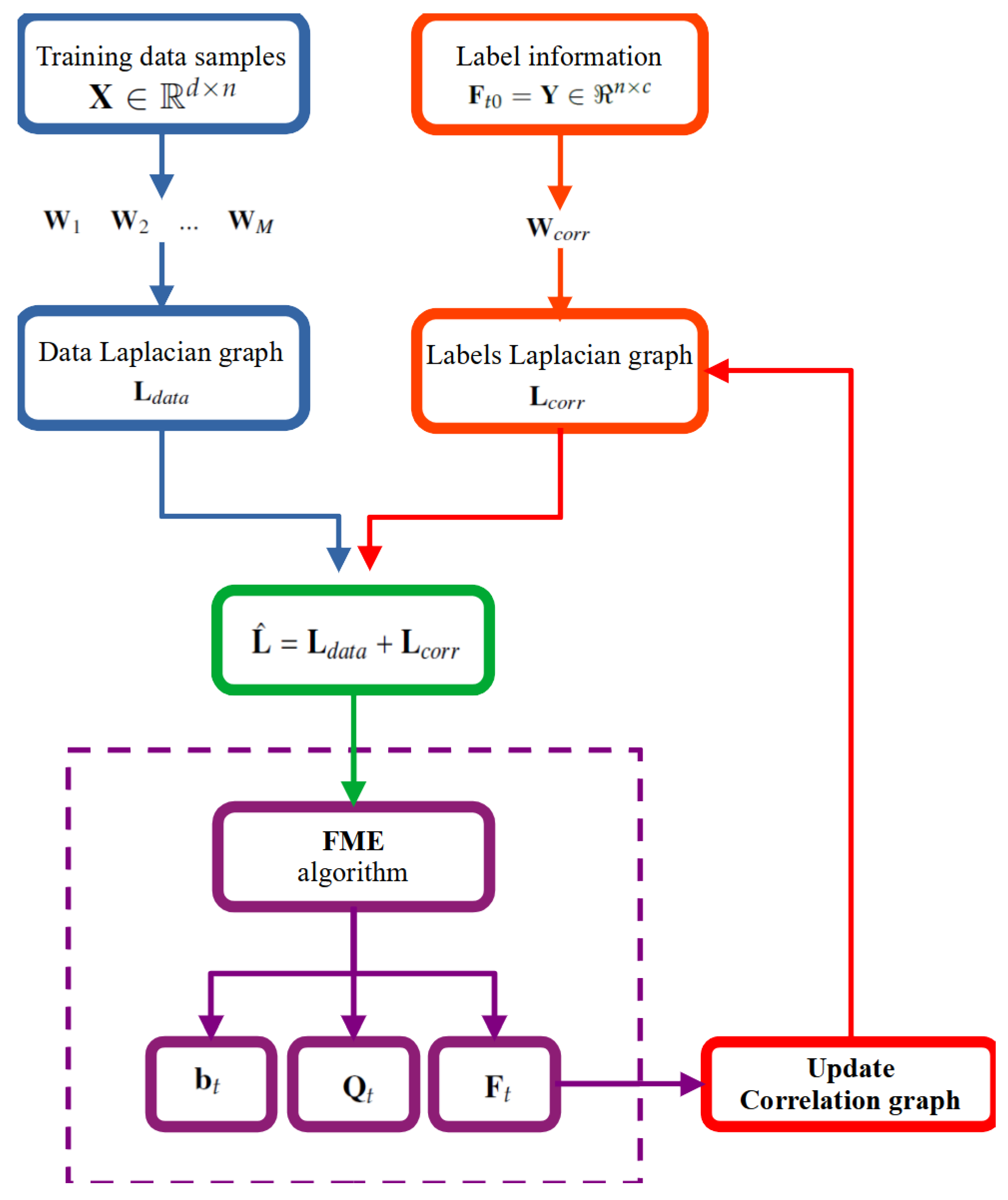
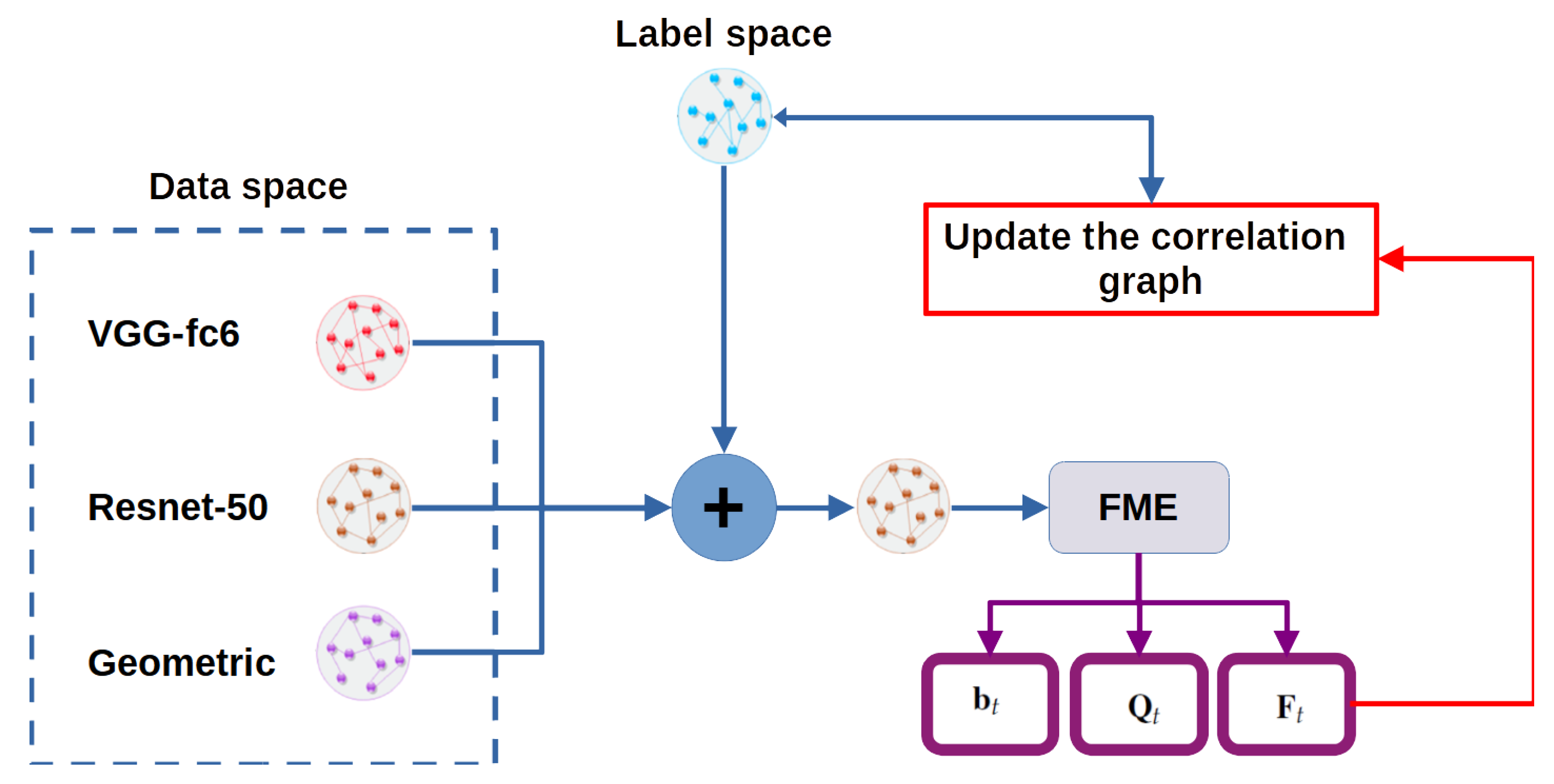
3.3. Proposed Algorithm
| Algorithm 1: Multi similarity metric fusion manifold embedding for face beauty prediction |
|
4. Experimental Results
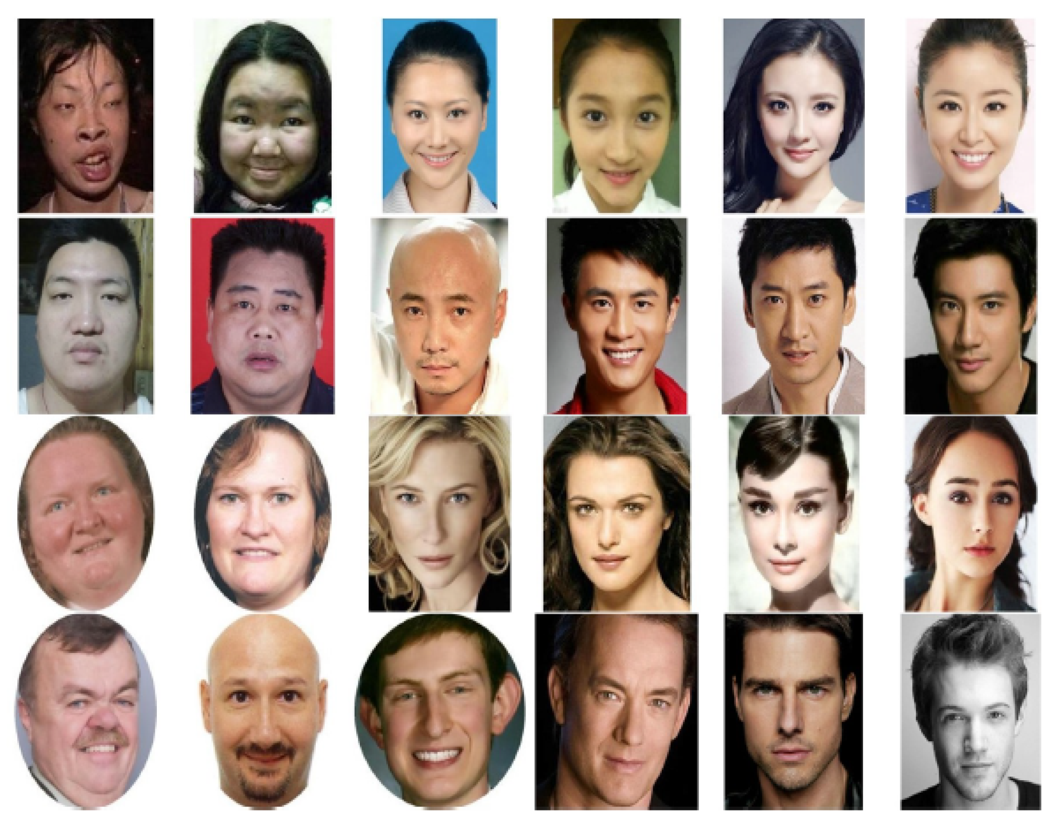
4.1. Databases
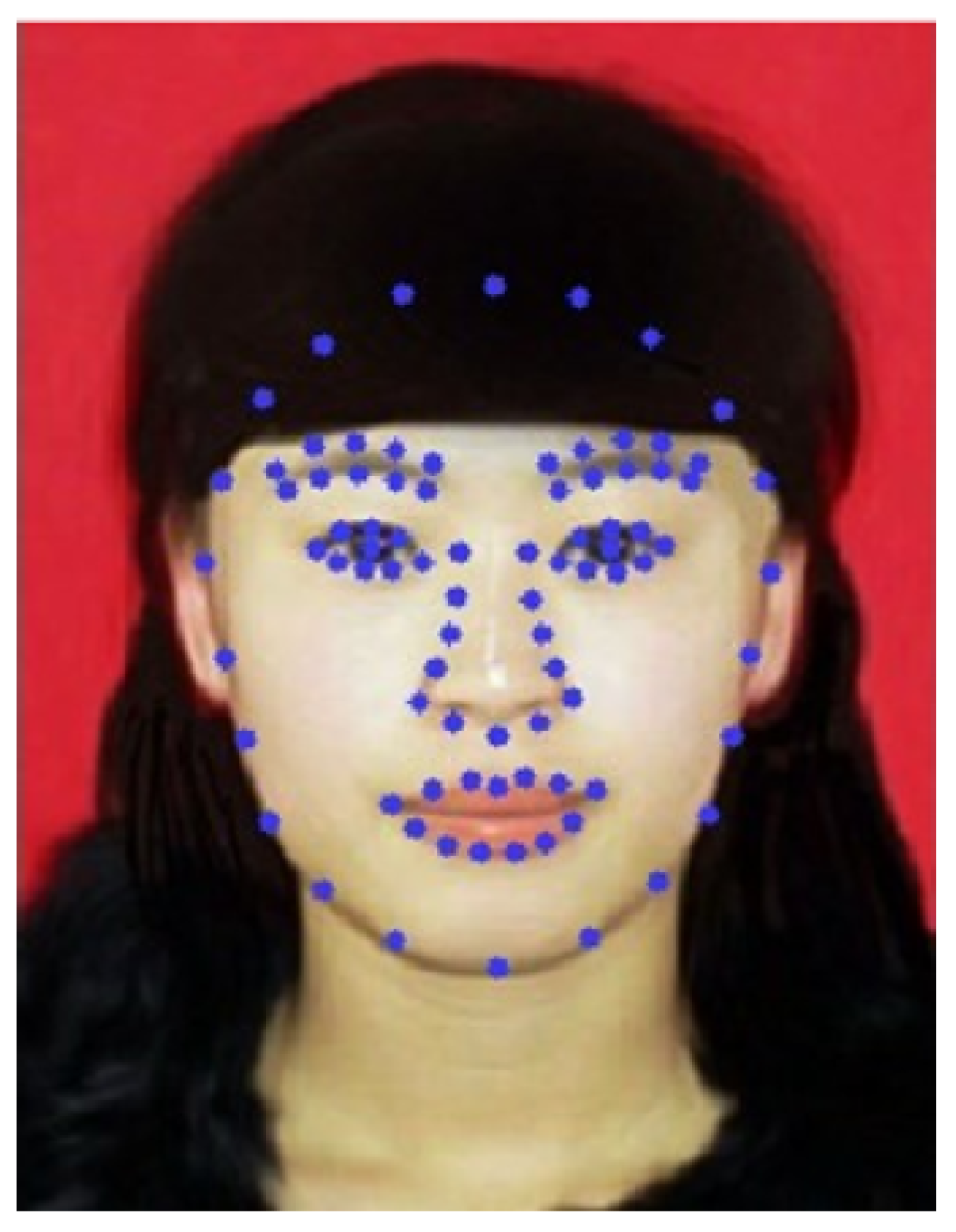
4.2. Features
4.3. Training Setup and Experimental Results
5. Conclusions
Author Contributions
Funding
Institutional Review Board Statement
Informed Consent Statement
Data Availability Statement
Conflicts of Interest
References
- Eco, U.; McEwen, A. History of Beauty; Rizzoli: New York, NY, USA, 2005. [Google Scholar]
- Kant, I. Critique of the Power of Judgment; The Cambridge Edition of the Works of Immanuel Kant, Cambridge University Press: Cambridge, UK, 2000. [Google Scholar] [CrossRef]
- Wolf, N. The Beauty Myth: How Images of Beauty Are Used against Women; Random House: New York, NY, USA, 2013. [Google Scholar]
- Chernorizov, A.M.; Zinchenko, Y.P.; Qing, J.Z.; Petrakova, A. Face cognition in humans: Psychophysiological, developmental, and cross-cultural aspects. Psychol. Russ. State Art 2016, 9, 37–50. [Google Scholar] [CrossRef]
- Eco, U. On Ugliness; Rizzoli: New York, NY, USA, 2007. [Google Scholar]
- Grammer, K.; Thornhill, R. Human (Homo sapiens) facial attractiveness and sexual selection: The role of symmetry and averageness. J. Comp. Psychol. 1994, 108, 233–242. [Google Scholar] [CrossRef] [PubMed]
- Rhodes, G.; Zebrowitz, L.A.; Clark, A.; Kalick, S.; Hightower, A.; McKay, R. Do facial averageness and symmetry signal health? Evol. Hum. Behav. 2001, 22, 31–46. [Google Scholar] [CrossRef]
- Perrett, D.I.; Lee, K.J.; Penton-Voak, I.; Rowland, D.; Yoshikawa, S.; Burt, D.M.; Henzi, S.P.; Castles, D.L.; Akamatsu, S. Effects of sexual dimorphism on facial attractiveness. Nature 1998, 394, 884–887. [Google Scholar] [CrossRef] [PubMed]
- Coetzee, V.; Perrett, D.I.; Stephen, I.D. Facial Adiposity: A Cue to Health? Perception 2009, 38, 1700–1711. [Google Scholar] [CrossRef]
- Matts, P.J.; Fink, B.; Grammer, K.; Burquest, M. Color homogeneity and visual perception of age, health, and attractiveness of female facial skin. J. Am. Acad. Dermatol. 2007, 57, 977–984. [Google Scholar] [CrossRef] [PubMed]
- de Jager, S.; Coetzee, N.; Coetzee, V. Facial Adiposity, Attractiveness, and Health: A Review. Front. Psychol. 2018, 9, 2562. [Google Scholar] [CrossRef] [Green Version]
- Richmond, S.; Howe, L.J.; Lewis, S.; Stergiakouli, E.; Zhurov, A. Facial Genetics: A Brief Overview. Front. Genet. 2018, 9, 462. [Google Scholar] [CrossRef] [Green Version]
- Zendle, D.; Meyer, R.; Ballou, N. The changing face of desktop video game monetisation: An exploration of exposure to loot boxes, pay to win, and cosmetic microtransactions in the most-played Steam games of 2010–2019. PLoS ONE 2020, 15, e0232780. [Google Scholar] [CrossRef]
- Hossam, M.; Afify, A.A.; Rady, M.; Nabil, M.; Moussa, K.; Yousri, R.; Darweesh, M.S. A Comparative Study of Different Face Shape Classification Techniques. In Proceedings of the 2021 International Conference on Electronic Engineering (ICEEM), Menouf, Egypt, 3–4 July 2021; pp. 1–6. [Google Scholar] [CrossRef]
- Gunes, H.; Piccardi, M. Assessing facial beauty through proportion analysis by image processing and supervised learning. Int. J. Hum.-Comput. Stud. 2006, 64, 1184–1199. [Google Scholar] [CrossRef] [Green Version]
- Langlois, J.H.; Roggman, L.A. Attractive Faces Are Only Average. Psychol. Sci. 1990, 1, 115–121. [Google Scholar] [CrossRef]
- Schölkopf, B.; Platt, J.; Hofmann, T. A Humanlike Predictor of Facial Attractiveness. In Advances in Neural Information Processing Systems 19: Proceedings of the 2006 Conference; MIT Press: Cambridge, MA, USA, 2007; pp. 649–656. [Google Scholar]
- Zhang, D.; Zhao, Q.; Chen, F. Quantitative analysis of human facial beauty using geometric features. Pattern Recognit. 2011, 44, 940–950. [Google Scholar] [CrossRef]
- Eisenthal, Y.; Dror, G.; Ruppin, E. Facial attractiveness: Beauty and the machine. Neural Comput. 2006, 18, 119–142. [Google Scholar] [CrossRef] [PubMed]
- Gray, D.; Yu, K.; Xu, W.; Gong, Y. Predicting facial beauty without landmarks. In Proceedings of the Computer Vision–ECCV 2010, Crete, Greece, 5–11 September 2010; pp. 434–447. [Google Scholar]
- Liu, X.; Li, T.; Peng, H.; Ouyang, I.C.; Kim, T.; Wang, R. Understanding Beauty via Deep Facial Features. In Proceedings of the 2019 IEEE/CVF Conference on Computer Vision and Pattern Recognition Workshops (CVPRW), Long Beach, CA, USA, 16–20 June 2019; pp. 246–256. [Google Scholar] [CrossRef] [Green Version]
- Gan, J.; Li, L.; Zhai, Y.; Liu, Y. Deep self-taught learning for facial beauty prediction. Neurocomputing 2014, 144, 295–303. [Google Scholar] [CrossRef]
- Wang, S.; Shao, M.; Fu, Y. Attractive or not?: Beauty prediction with attractiveness-aware encoders and robust late fusion. In Proceedings of the 22nd ACM International Conference on Multimedia, Orlando, FL, USA, 3–7 November 2014; ACM: New York, NY, USA, 2014; pp. 805–808. [Google Scholar]
- Nguyen, T.V.; Liu, S.; Ni, B.; Tan, J.; Rui, Y.; Yan, S. Towards decrypting attractiveness via multi-modality cues. ACM Trans. Multimed. Comput. Commun. Appl. (TOMM) 2013, 9, 28. [Google Scholar] [CrossRef]
- Xie, D.; Liang, L.; Jin, L.; Xu, J.; Li, M. SCUT-FBP: A benchmark dataset for facial beauty perception. In Proceedings of the 2015 IEEE International Conference on Systems, Man, and Cybernetics (SMC), Hong Kong, China, 9–12 October 2015; pp. 1821–1826. [Google Scholar]
- Xu, J.; Jin, L.; Liang, L.; Feng, Z.; Xie, D. A new humanlike facial attractiveness predictor with cascaded fine-tuning deep learning model. arXiv 2015, arXiv:1511.02465. [Google Scholar]
- Dornaika, F.; Bosaghzadeh, A. Exponential Local Discriminant Embedding and Its Application to Face Recognition. IEEE Trans. Cybern. 2013, 43, 921–934. [Google Scholar] [CrossRef]
- Dornaika, F.; Elorza, A.; Wang, K.; Arganda-Carreras, I. Nonlinear, flexible, semisupervised learning scheme for face beauty scoring. J. Electron. Imaging 2019, 28, 1. [Google Scholar] [CrossRef]
- Dornaika, F.; Wang, K.; Arganda-Carreras, I.; Elorza, A.; Moujahid, A. Toward graph-based semi-supervised face beauty prediction. Expert Syst. Appl. 2020, 142, 112990. [Google Scholar] [CrossRef]
- El Traboulsi, Y.; Dornaika, F.; Assoum, A. Kernel flexible manifold embedding for pattern classification. Neurocomputing 2015, 167, 517–527. [Google Scholar] [CrossRef]
- Nie, F.; Xu, D.; Tsang, I.W.H.; Zhang, C. Flexible Manifold Embedding: A Framework for Semi-Supervised and Unsupervised Dimension Reduction. IEEE Trans. Image Process. 2010, 19, 1921–1932. [Google Scholar] [CrossRef] [PubMed]
- An, L.; Chen, X.; Yang, S. Multi-graph feature level fusion for person re-identification. Neurocomputing 2017, 259, 39–45. [Google Scholar] [CrossRef]
- Ziraki, N.; Dornaika, F.; Bosaghzadeh, A. Multiple-view flexible semi-supervised classification through consistent graph construction and label propagation. Neural Netw. 2022, 146, 174–180. [Google Scholar] [CrossRef] [PubMed]
- Namjoy, A.; Bosaghzadeh, A. A Sample Dependent Decision Fusion Algorithm for Graph-based Semi-supervised Learning. Int. J. Eng. 2020, 33, 1010–1019. [Google Scholar] [CrossRef]
- Dornaika, F.; Dahbi, R.; Bosaghzadeh, A.; Ruichek, Y. Efficient dynamic graph construction for inductive semi-supervised learning. Neural Netw. 2017, 94, 192–203. [Google Scholar] [CrossRef]
- Karasuyama, M.; Mamitsuka, H. Multiple Graph Label Propagation by Sparse Integration. IEEE Trans. Neural Netw. Learn. Syst. 2013, 24, 1999–2012. [Google Scholar] [CrossRef]
- Lin, G.; Liao, K.; Sun, B.; Chen, Y.; Zhao, F. Dynamic graph fusion label propagation for semi-supervised multi-modality classification. Pattern Recognit. 2017, 68, 14–23. [Google Scholar] [CrossRef]
- Wang, B.; Tsotsos, J. Dynamic label propagation for semi-supervised multi-class multi-label classification. Pattern Recognit. 2016, 52, 75–84. [Google Scholar] [CrossRef]
- Zhang, L.; Zhang, D. MetricFusion: Generalized Metric Swarm Learning for Similarity Measure. Inf. Fusion 2016, 30, 80–90. [Google Scholar] [CrossRef]
- Cao, Q.; Ying, Y.; Li, P. Similarity Metric Learning for Face Recognition. In Proceedings of the IEEE International Conference on Computer Vision (ICCV), Sydney, Australia, 1–8 December 2013. [Google Scholar]
- Zhang, Y.; Zhang, H.; Nasrabadi, N.M.; Huang, T.S. Multi-metric learning for multi-sensor fusion based classification. Inf. Fusion 2013, 14, 431–440. [Google Scholar] [CrossRef]
- Zhou, D.; Bousquet, O.; Lal, T.; Weston, J.; Schölkopf, B. Learning with Local and Global Consistency. In Advances in Neural Information Processing Systems; Thrun, S., Saul, L., Schölkopf, B., Eds.; MIT Press: Cambridge, MA, USA, 2003; Volume 16. [Google Scholar]
- Bahrami, S.; Bosaghzadeh, A.; Dornaika, F. Multi Similarity Metric Fusion in Graph-Based Semi-Supervised Learning. Computation 2019, 7, 15. [Google Scholar] [CrossRef] [Green Version]
- Eppstein, D.; Paterson, M.; Yao, F. On Nearest-Neighbor Graphs. Comput. Geom. 1997, 17, 263–282. [Google Scholar] [CrossRef] [Green Version]
- Manning, C.; Prabhakar, R.; Hinrich, S. “16. Flat Clustering”. Introduction to Information Retrieval; Cambridge University Press: New York, NY, USA, 2008. [Google Scholar]
- Saeed, J.N.; Abdulazeez, A.M. Facial Beauty Prediction and Analysis Based on Deep Convolutional Neural Network: A Review. J. Soft Comput. Data Min. 2021, 2, 1–12. [Google Scholar] [CrossRef]
- He, K.; Zhang, X.; Ren, S.; Sun, J. Deep Residual Learning for Image Recognition. In Proceedings of the 2016 IEEE Conference on Computer Vision and Pattern Recognition (CVPR), Las Vegas, NV, USA, 27–30 June 2016; pp. 770–778. [Google Scholar]
- Parkhi, O.M.; Vedaldi, A.; Zisserman, A. Deep Face Recognition. In Proceedings of the BMVC 2015, Swansea, UK, 7–10 September 2015; Volume 1, p. 6. [Google Scholar]
- Liang, L.; Lin, L.; Jin, L.; Xie, D.; Li, M. SCUT-FBP5500: A diverse benchmark dataset for multi-paradigm facial beauty prediction. In Proceedings of the 2018 24th International Conference on Pattern Recognition (ICPR), Beijing, China, 20–24 August 2018; pp. 1598–1603. [Google Scholar]
- Cao, K.; Choi, K.n.; Jung, H.; Duan, L. Deep Learning for Facial Beauty Prediction. Information 2020, 11, 391. [Google Scholar] [CrossRef]
- Xu, J.; Jin, L.; Liang, L.; Feng, Z.; Xie, D.; Mao, H. Facial attractiveness prediction using psychologically inspired convolutional neural network (PI-CNN). In Proceedings of the 2017 IEEE International Conference on Acoustics, Speech and Signal Processing (ICASSP), New Orleans, LA, USA, 5–9 March 2017; pp. 1657–1661. [Google Scholar]
- Fan, Y.Y.; Liu, S.; Li, B.; Guo, Z.; Samal, A.; Wan, J.; Li, S.Z. Label distribution-based facial attractiveness computation by deep residual learning. IEEE Trans. Multimed. 2017, 20, 2196–2208. [Google Scholar] [CrossRef] [Green Version]
- Lin, L.; Liang, L.; Jin, L.; Chen, W. Attribute-Aware Convolutional Neural Networks for Facial Beauty Prediction. In Proceedings of the International Joint Conference on Artificial Intelligence (IJCAI), Macao, China, 10–16 August 2019; pp. 847–853. [Google Scholar]
- Lin, L.; Liang, L.; Jin, L. Regression guided by relative ranking using convolutional neural network (R3CNN) for facial beauty prediction. IEEE Trans. Affect. Comput. 2019, 13, 122–134. [Google Scholar] [CrossRef]
- Langlois, J.H.; Kalakanis, L.; Rubenstein, A.J.; Larson, A.; Hallam, M.; Smoot, M. Maxims or myths of beauty? A meta-analytic and theoretical review. Psychol. Bull. 2000, 126, 390–423. [Google Scholar] [CrossRef]
- Cunningham, M.R.; Roberts, A.R.; Barbee, A.P.; Druen, P.B.; Wu, C.H. “Their ideas of beauty are, on the whole, the same as ours”: Consistency and variability in the cross-cultural perception of female physical attractiveness. J. Personal. Soc. Psychol. 1995, 68, 261. [Google Scholar] [CrossRef]
- Wald, C. Beauty: 4 big questions. Nature 2015, 526, S17. [Google Scholar] [CrossRef] [Green Version]
- Wald, C. Neuroscience: The aesthetic brain. Nature 2015, 526, S2–S3. [Google Scholar] [CrossRef]


| Notation | Description |
|---|---|
| Training data samples | |
| ℓ | Number of labelled samples |
| u | Number of unlabelled samples () |
| d | Dimensionality of data |
| n | Number of training samples/images |
| C | Total number of classes |
| Prediction label matrix or Prediction score vector | |
| Binary label matrix or ground-truth score vector | |
| Indicator diagonal Matrix | |
| Projection Matrix or Projection vector | |
| Bias vector or bias scalar |
| Dataset | Descriptor | Dimension | # of Instance |
|---|---|---|---|
| SCUT5500-AF | VGG-face+fc6 | 4096 | 2000 |
| Resnet50 | 2048 | ||
| Geometric | 162 | ||
| SCUT5500-AM | VGG-face+fc6 | 4096 | 2000 |
| Resnet50 | 2048 | ||
| Geometric | 162 | ||
| SCUT5500-CF | VGG-face+fc6 | 4096 | 750 |
| Resnet50 | 2048 | ||
| Geometric | 162 | ||
| SCUT5500-CM | VGG-face+fc6 | 4096 | 750 |
| Resnet50 | 2048 | ||
| Geometric | 162 |
| Dataset | Method | MAE ↓ | RMSE ↓ | PC (%) ↑ |
|---|---|---|---|---|
| SCUT5500-AF | VGG-face+fc6 | 0.237 | 0.307 | 89.4 |
| ResNet-50 | 0.225 | 0.300 | 90.5 | |
| Proposed method | 0.220 | 0.277 | 91.3 | |
| SCUT5500-AM | VGG-face+fc6 | 0.232 | 0.301 | 89.9 |
| ResNet-50 | 0.224 | 0.283 | 91.5 | |
| Proposed method | 0.218 | 0.276 | 92.2 | |
| SCUT5500-CF | VGG-face+fc6 | 0.257 | 0.337 | 88.6 |
| ResNet-50 | 0.241 | 0.324 | 89.5 | |
| Proposed method | 0.231 | 0.302 | 90.3 | |
| SCUT5500-CM | VGG-face+fc6 | 0.234 | 0.318 | 88.7 |
| ResNet-50 | 0.232 | 0.317 | 89.9 | |
| Proposed method | 0.230 | 0.300 | 90.5 | |
| SCUT5500 | VGG-face+fc6 | 0.242 | 0.317 | 89.0 |
| ResNet-50 | 0.229 | 0.302 | 90.2 | |
| Proposed method | 0.221 | 0.2870 | 91.1 |
| Method | MAE ↓ | RMSE ↓ | PC (%) ↑ |
|---|---|---|---|
| Alexnet [49] | 0.2651 | 0.3481 | 86.34 |
| Resnet-18 [49] | 0.2419 | 0.3166 | 89.00 |
| ResneXt-50 [49] | 0.2291 | 0.3017 | 89.97 |
| CNN with SCA [50] | 0.2287 | 0.3014 | 90.03 |
| PI-CNN [51] | 0.2267 | 0.3016 | 89.78 |
| CNN + LDL [52] | 0.2201 | 0.2940 | 90.31 |
| ResNet-18 based AaNet [53] | 0.2236 | 0.2954 | 90.55 |
| ResneXt-50-R3CNN [54] | 0.2120 | 0.2800 | 91.42 |
| Semi-supervised [29] | 0.2675 | 0.3455 | 86.60 |
| Semi-supervised (Ours) | 0.2210 | 0.2870 | 91.13 |
Publisher’s Note: MDPI stays neutral with regard to jurisdictional claims in published maps and institutional affiliations. |
© 2022 by the authors. Licensee MDPI, Basel, Switzerland. This article is an open access article distributed under the terms and conditions of the Creative Commons Attribution (CC BY) license (https://creativecommons.org/licenses/by/4.0/).
Share and Cite
Dornaika, F.; Moujahid, A. Multi-View Graph Fusion for Semi-Supervised Learning: Application to Image-Based Face Beauty Prediction. Algorithms 2022, 15, 207. https://doi.org/10.3390/a15060207
Dornaika F, Moujahid A. Multi-View Graph Fusion for Semi-Supervised Learning: Application to Image-Based Face Beauty Prediction. Algorithms. 2022; 15(6):207. https://doi.org/10.3390/a15060207
Chicago/Turabian StyleDornaika, Fadi, and Abdelmalik Moujahid. 2022. "Multi-View Graph Fusion for Semi-Supervised Learning: Application to Image-Based Face Beauty Prediction" Algorithms 15, no. 6: 207. https://doi.org/10.3390/a15060207
APA StyleDornaika, F., & Moujahid, A. (2022). Multi-View Graph Fusion for Semi-Supervised Learning: Application to Image-Based Face Beauty Prediction. Algorithms, 15(6), 207. https://doi.org/10.3390/a15060207