Article

BAG-DSM: A Method for Generating Alternatives for Hierarchical Multi-Attribute Decision Models Using Bayesian Optimization

by
Martin Gjoreski
1,*,
Vladimir Kuzmanovski
2 and
Marko Bohanec
3
1
Faculty of Informatics, Università della Svizzera Italiana (USI), Via Giuseppe Buffi 13, CH-6900 Lugano, Switzerland
2
Department of Computer Science, Aalto University, FI-00076 Aalto, Finland
3
Department of Knowledge Technologies, Jožef Stefan Institute, Jamova Cesta 39, SI-1000 Ljubljana, Slovenia
*
Author to whom correspondence should be addressed.
Algorithms 2022, 15(6), 197; https://doi.org/10.3390/a15060197
Submission received: 6 May 2022 / Revised: 2 June 2022 / Accepted: 3 June 2022 / Published: 7 June 2022
(This article belongs to the Special Issue Algorithms in Decision Support Systems Vol. 2)

Abstract

:
Multi-attribute decision analysis is an approach to decision support in which decision alternatives are evaluated by multi-criteria models. An advanced feature of decision support models is the possibility to search for new alternatives that satisfy certain conditions. This task is important for practical decision support; however, the related work on generating alternatives for qualitative multi-attribute decision models is quite scarce. In this paper, we introduce Bayesian Alternative Generator for Decision Support Models (BAG-DSM), a method to address the problem of generating alternatives. More specifically, given a multi-attribute hierarchical model and an alternative representing the initial state, the goal is to generate alternatives that demand the least change in the provided alternative to obtain a desirable outcome. The brute force approach has exponential time complexity and has prohibitively long execution times, even for moderately sized models. BAG-DSM avoids these problems by using a Bayesian optimization approach adapted to qualitative DEX models. BAG-DSM was extensively evaluated and compared to a baseline method on 43 different DEX decision models with varying complexity, e.g., different depth and attribute importance. The comparison was performed with respect to: the time to obtain the first appropriate alternative, the number of generated alternatives, and the number of attribute changes required to reach the generated alternatives. BAG-DSM outperforms the baseline in all of the experiments by a large margin. Additionally, the evaluation confirms BAG-DSM’s suitability for the task, i.e., on average, it generates at least one appropriate alternative within two seconds. The relation between the depth of the multi-attribute hierarchical models—a parameter that increases the search space exponentially—and the time to obtaining the first appropriate alternative was linear and not exponential, by which BAG-DSM’s scalability is empirically confirmed.

1. Introduction

Decision support systems (DSSs) are interactive information systems intended to help decision makers utilize data and models in order to identify and solve problems and make decisions [1,2,3]. Typically, decision support models are static and provide the users with an output for a given input (Step 1 and Step 2 in Figure 1). However, besides the output, users are often interested in alternatives that are close to their initial input and enable a change, usually a positive one, in the output of the model (see Step 1 and Step 2—with BAG-DSM in Figure 1). To solve that specific problem, we developed BAG-DSM, a surrogate-based stochastic optimization method for searching the decision space and generating alternatives that fulfill certain criteria with regard to the provided initial state (current alternative) and that guarantees evaluation of the outcome to the desired level.
Hierarchical multi-attribute models are a type of decision model used in DSSs that decompose the problem into smaller and less complex subproblems and represent it by a hierarchy of attributes and utility or aggregation functions. Such decision models are especially useful in solving complex decision problems [4,5,6,7]. DEX [8] is a qualitative hierarchical multi-attribute method whose models are characterized by using qualitative (symbolic) attributes and decision rules. The method is supported by DEXi [8], an interactive computer program for the development of qualitative multi-attribute decision models and the evaluation of alternatives. DEXi has been used to analyze decision problems in different domains. According to [8], DEXi was used in healthcare for the assessment of breast cancer risk, assessment of basic living activities in community nursing, risk assessment in diabetic foot care, and advising about medication therapy for Parkinson’s disease. In agriculture, DEXi [8] was used for assessing the impact of cropping systems on soil quality, assessing the ecological and the economic impact of genetically modified crops, assessing livestock systems, and predicting insect pest damage to crops. Some other recent applications were carried out in the fields of electricity production [9], risk assessment [10], sustainability development [11], and knowledge management [12].
Besides modeling expert knowledge and evaluating existing alternatives, DEXi can be used for what-if analysis, i.e., the process of changing the values of certain attributes in an existing alternative and analyzing how those changes affect the outcome. The what-if analysis has the ability to investigate the differences within a given set of alternatives but lacks the ability to generate the alternative set itself. The provided set of alternatives comprises alternatives that the decision maker chooses to investigate based on corresponding expert knowledge about the underlying decision problem and the set of attributes. However, imposing a condition to consider the desired evaluation of the outcome, which differs from the actual evaluation, makes the what-if analysis intractable.
Therefore, a useful extension of such analysis would be to provide the possibility to search for new alternatives or to generate them under a certain set of conditions that strongly relate to or depend on the initial or current state of the modeled system in order to obtain a desirable outcome—an evaluation of the modeled phenomenon. The solutions should satisfy the criteria of least deviation from the initial state, where the deviation is defined with a geometric or set-based distance measure(s) from a given alternative (initial state). This task is important for practical decision support.
The qualitative nature of DEX models, along with the set of input attributes and their domains (sets of nominal values that each attribute receives a value from), defines the combinatorial nature of the underlying search task that evolves in a complex combinatorial optimization problem, where the dimensionality of its search space affects the complexity. A trivial approach to the given search problem is an application of the brute-force or exhaustive search algorithm. However, the brute-force approach that evaluates all possible alternatives is computationally demanding and not reasonable for sufficiently large models. For example, for a decision model with 20 input attributes and cardinality of their value sets (scales) equal to three (e.g., “low”, “medium”, “high”), the number of possible alternatives (candidate solutions) is 320, i.e., close to 3.5 × 10⁹. Consequently, more advanced search methods in terms of intelligence and efficiency in traversing the search space are required to avoid the combinatorial explosion.
The contribution that this paper presents is the novel method Bayesian Alternative Generator for Decision Support Models (BAG-DSM), which aids the search through the decision space of DEX decision support models. The approach uses Bayesian optimization and its utility to investigate the tradeoff between exploration and exploitation of unknown regions and reached discoveries, respectively. BAG-DSM was evaluated on 42 qualitative multi-attribute models with varying complexity. BAG-DSM’s behavior and performance are analyzed with respect to several characteristics, including computational time, time to finding the first appropriate alternative, the number of generated (appropriate) alternatives, and the number of attribute changes required to reach the generated alternatives.
The rest of the paper is structured as follows: Section 2 presents the related work. Section 3 presents the theoretical background of multi-criteria decision analysis with a focus on DEX methodology. Section 4 presents the proposed BAG-DSM, including theoretical and implementation details. Section 5 presents the experimental setup and the experimental results. Section 6 discusses the results, including limitations, future work, and implications related to BAG-DSM. Finally, Section 7 concludes the paper.

2. Related Work

Most of the studies that analyze alternatives in multi-attribute decision models focus on the development of methods for ranking alternatives [13,14]. These methods are useful in use cases when the expert needs to choose one alternative from a set of possible alternatives. However, in use cases where the set of possible alternatives is not predefined, such methods are not applicable. Furthermore, such ranking methods lack the ability to generate new alternatives, leading to the desired outcome, which satisfies a set of criteria strongly related to and dependent on the initial or present state of the modeled system—the current alternative.
The related work on generating an alternative for multi-attribute decision models, particularly qualitative models such as DEX, is quite scarce. The only related study known to the authors was presented by Bergez [15], in which the focus is on attribute scoring (and not on the alternatives), and a given (current) alternative was not taken into consideration. More specifically, Bergez developed a genetic algorithm for searching a set of the “worst-best”, i.e., lowest scores for the input attributes that lead to the highest score for the root attribute (the decision model’s output), and “best-worst”, i.e., highest scores for the input attributes that lead to the lowest score for the root attribute. Bergez’s use case involves a complex model for ex ante assessment of the sustainability of cropping systems and provides an excellent justification for using such methods in decision support.
Generating candidate alternatives that would change the model’s output is also a problem faced by the machine learning (ML) community, thanks to the recent changes related to the EU’s General Data Protection Regulation (GDPR). According to GDPR, the ML models should offer the possibility to answer/provide an explanation such as: “You were denied a loan because your annual income was £30,000. If your income had been £45,000, you would have been offered a loan” [16]. This new regulation prompted the ML community to explore the explainability of ML models to the extent that some researchers argue that the model’s accuracy should be sacrificed and interpretable models should be preferred over black-box ML models for high-stakes decisions [17].
In the ML domain, this task is referred to as a search for counterfactual explanations. The idea is that, besides the model’s output, additional counterfactual information should be provided on how the world would have to be different for a desirable outcome to occur. Wachter et al. [16] presented examples of how meaningful counterfactuals can be computed for standard weight-based ML algorithms, e.g., neural networks, support vector machines, and logistic repressors. The proposed BAG-DSM utilizes the models’ weights and a specific distance function to search for counterfactuals. Joshi et al. [18] presented a method that first learns a latent space of the training data using a variational autoencoder based on neural networks and then uses the latent space to search for the counterfactual explanations. While quite powerful, both of these methods are weight- and gradient-based and require a differentiable distance function, which is not always available with multi-attribute decision models and is especially limited in qualitative domains. Karimi et al. [19] proposed a general method based on first-order predicate logic to generate the nearest counterfactual explanations. They evaluated their approach using predictive models such as decision trees, random forest, logistic regression, and multilayer perceptron. Wexler et al. [20] presented a method that searches in the training data for the closest sample that flips the model’s prediction. Tolomei et al. [21] presented an approach that searches for the nearest counterfactual close to the decision boundary of a random forest model. Ustun et al. [22] presented a method that solves a mixed-integer linear program to obtain counterfactual explanations for linear regression models. However, these ML-based studies have limited ability to handle discrete utility functions, which are a base in our study for qualitative multi-attribute decision models.

3. Problem Description

3.1. Multi-Criteria Modeling
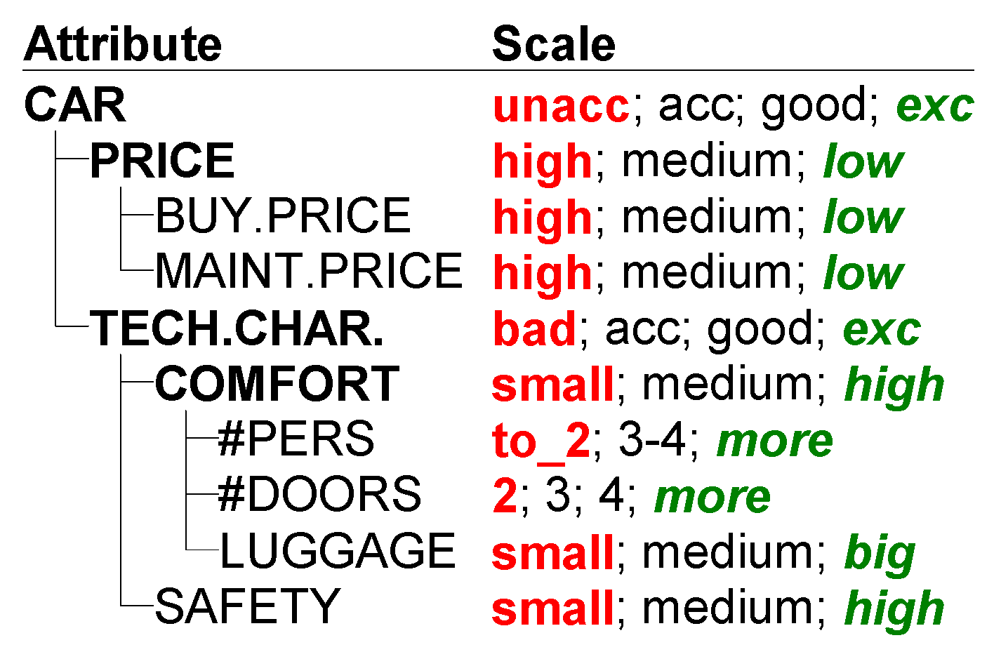
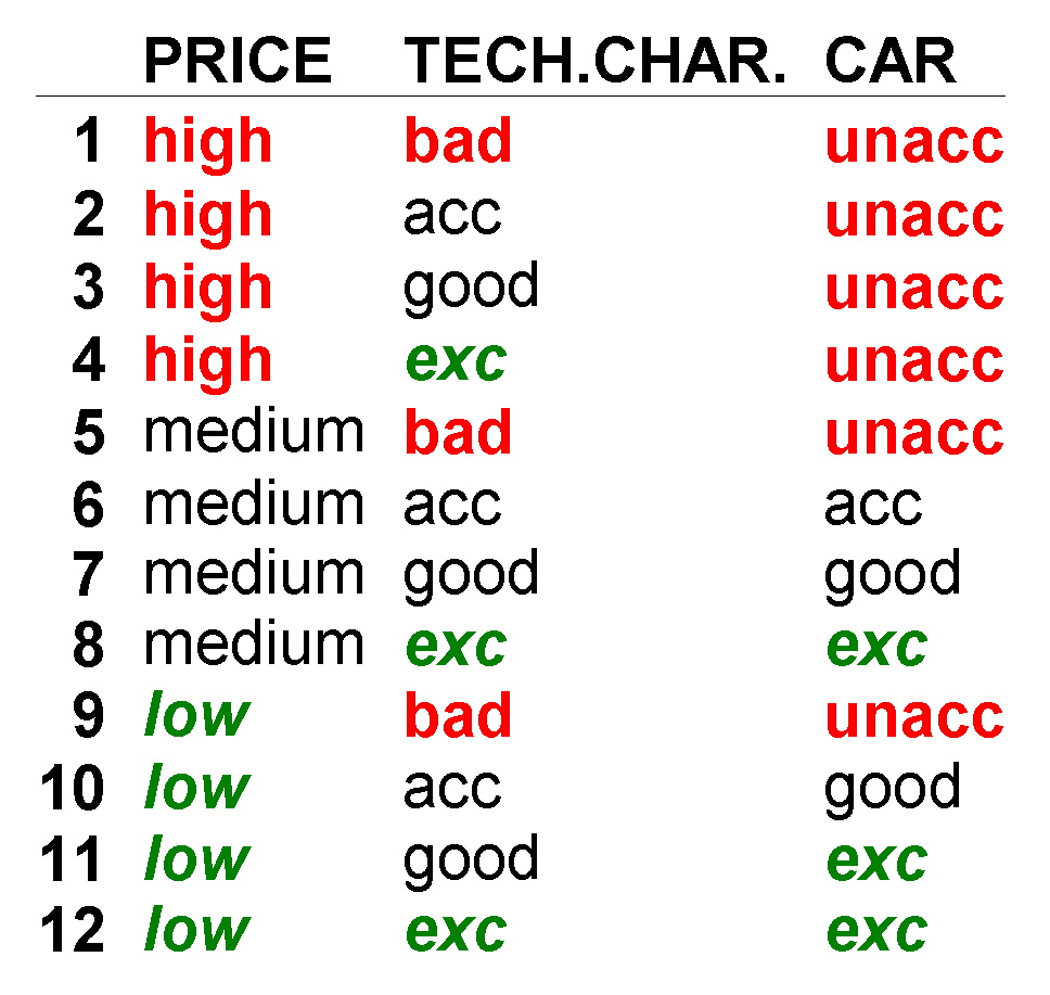
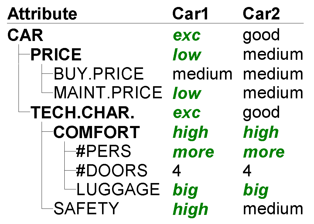
Multi-criteria decision analysis (MCDM) [6] is an approach to decision support that explicitly considers multiple and possibly conflicting criteria for assessing decision alternatives. One of the central MCDM concepts is a notion of a multi-criteria (or multi-attribute) model, which is aimed at capturing the decision maker’s preferences and goals, and eventually creating means to evaluate and analyze decision alternatives in a numerical or qualitative way. At the surface, an MCDM model can be seen as an aggregation function,
U = F x 1 , x 2 , , x n ,
that evaluates decision alternatives, which are represented by the values of multiple criteria x i ,   i = 1 , 2 , , n . The variables x i usually represent some observable properties of alternatives that influence the decision, such as cost, performance, or economy. The aggregation yields an overall evaluation (utility) U , which is used as a measure to rank alternatives and/or to select the optimal (preferred) one. MCDM provides a multitude of methods that use different internal representations of F and differ in the ways F is acquired from the decision maker and how it is used to support various decision-making tasks. Let us also add that the majority of MCDM methods rely on linear models of the form
U = w 1 x 1 + w 2 x 2 + + w n x n
where w i ,   i = 1 , 2 , , n are weights representing the relative importance of criteria.

3.2. Method DEX

Decision expert (DEX) [8] is an MCDM method that takes the same model aggregation approach; however, it departs from the mainstream MCDM methods by using qualitative rather than numeric criteria. Criteria x i in DEX are represented by variables (called attributes) that take values that are usually represented by words, such as “bad”, “acceptable”, “high”. The aggregation of such values into an overall U , which is also qualitative, is in DEX governed by decision rules rather than by the weighted sum or some other form of numerical aggregation. The DEX method was motivated by the needs of problem domains that involve inaccurate or even missing data and require judgment and qualitative knowledge-based reasoning. DEX is particularly suitable for supporting sorting decision problems [23], where the goal is to assign decision alternatives into ordered and predefined groups, called categories.
Example 1.
As an introductory example of DEX, let us use a simple model for the evaluation of vehicles, which is distributed together with the DEXi software. The model consists of six basic attributes (BUY.PRICE, MAINT.PRICE, #PERS, #DOORS, LUGGAGE, and SAFETY), which are used as inputs to the model. The model has a hierarchical structure (Figure 2). Input attributes are gradually aggregated through three aggregate attributes (PRICE, COMFORT, and TECH.CHAR.). The root of the tree, called CAR, represents the overall evaluation of decision alternatives—cars. Figure 3 also shows the value scales of attributes, illustrating the use of words (such as “small”, “medium”, “big”). These words are generally ordered by preference from “bad” to “good” values, and the red and green colors denote particularly bad and good individual values, respectively.
The aggregation in DEX is defined by decision tables consisting of decision rules. Figure 3 shows the topmost table in the CAR model, which aggregates the lower-level attributes PRICE and TECH.CHAR. to the final CAR evaluation. Each row in the table represents a simple decision rule; for instance, row 4:
if PRICE = “high” and TECH.CHAR. = “exc” then CAR = “unacc(eptable)”.
Such decision tables are usually defined by the decision maker and are meant to reflect their preferences. In addition to the rules in Figure 2, the CAR model contains three more decision tables, not shown here, that correspond to the aggregate attributes PRICE, TECH.CHAR., and COMFORT.
The CAR model, consisting of the attributes (Figure 2) and decision tables (one shown in Figure 3), collectively represents the aggregation
CAR = F(BUY.PRICE, MAINT.PRICE, #PERS, #DOORS, LUGGAGE, SAFETY),
where F is the aggregation function defined by decision rules. The six arguments of F are variables representing observable properties of cars, and CAR is the overall evaluation of a car, represented by categories “unacc”, “acc”, “good”, “exc”. This function can be used to evaluate specific vehicles, as illustrated in Figure 4.
In this study, we are interested in the following type of question: Consider Car2 in Figure 4. What can we do to improve its overall evaluation from CAR = “good” to CAR = “exc”? In which way should we change BUY.PRICE, MAINT.PRICE, and/or any combination of input values in order to achieve that goal? Apparently, this is a combinatorial problem, which is not particularly difficult for simple models such as CAR. One may notice that the inputs to CAR consist of five attributes that can take three qualitative values and one attribute (#DOORS) that can take four values. In this way, the input space consists of 3 × 3 × 3 × 3 × 3 × 4 = 972 possible value combinations, which can all be easily evaluated by an exhaustive algorithm. However, the latter becomes impossible with larger and more complex models.
Example 2.
Here we take a larger, more complex, but realistic DEX model in the domain of agriculture [24]. The model, whose structure is shown in Figure 5, is aimed at assessing the primary productivity of agricultural fields by considering soil properties, environmental aspects, crop properties, and management options. The description of the model is beyond the scope of this paper; however, it is included here to illustrate two important points. First, after evaluating an agricultural field and assessing its primary productivity, a caring farmer would ask questions such as: What can I do to improve productivity? What can go wrong and degrade productivity? Such questions are highly relevant and should be supported by appropriate methods and algorithms. Second, this model has 26 input attributes and, consequently, a huge input space: 2 4 × 3 18 × 4 4 1.59 × 10 12 . The exhaustive search for solutions is clearly unfeasible, and more efficient algorithms are needed to solve the problem in a realistic time frame.

3.3. DEX Models and Their Properties

This study comprises DEX models that allow investigating performances of the proposed BAG-DSM for generating alternatives yet give a clear insight into the applicability of the BAG-DSM on decision problems bounded by real-world settings, such as the second example above. Therefore, along with the decision model for assessing the capacity of primary productivity soil function presented above, the study includes a set of artificial (benchmark) DEX multi-attribute decision models.
The benchmark DEX models are designed by Kuzmanovski et al. [25]. In this study, they are used for benchmarking the methods’ performances with respect to varying properties of the decision model and, hence, the decision problem. They encompass trivial structures, with unified attributes with regard to their value scales (Figure 6a). The set has 42 DEX models and exhibits variation in three model properties that define the overall complexity of a decision problem: (i) distribution of attributes’ aggregation weights (weight distribution), (ii) depth of the hierarchical structure (model depth), and (iii) inter-dependency of input attributes.
The aggregation weights resemble the idea of other MCDA methods that linearly combine attribute values, but with no explicit definition of such weights. Instead, the weights in DEX are either defined explicitly by the decision maker or implicitly derived from the decision rules, which do not necessarily exhibit a linear relation. Following the paradigm of the linear models, where weights explain the extent of variability in outcomes, the weights’ distribution considerably influences the ability to quickly generate a suitable alternative, i.e., determines the bounds of the search space. However, accurately estimating such weights and their distribution is not trivial. Therefore, for benchmark models, Kuzmanovski et al. [25] defined three classes of weight distributions: skewed, normal, and uniform, which express the distribution of weights in terms of dominant and tailing attributes across all aggregations in the DEX models. The skewed distribution of weights corresponds to the complete dominance of a single attribute, while the rest of the attributes have no influence in an aggregation (Figure 6b). Normal distribution resembles a tailed bell-shaped distribution with one attribute being dominant, while the rest have fewer (minor) effects in the aggregation (Figure 6c). Uniform distribution, as the name suggests, equally distributes the effect or influence of input attributes on the outcome of the aggregation (Figure 6d). The defined classes of skewed, normal, and uniform distributions of weights translate to small, medium, and large search spaces, respectively.
The depth of the DEX models shows the number of levels in their tree-like hierarchical structure, including the level of input attributes. The depth of the model, where at each aggregation, at least two attributes are combined, influences the number of input attributes. Therefore, depth influences the dimensionality of the search space (number of input attributes), and hence, the complexity of the decision problem. The set of benchmark DEX models includes models with the depth of 3, 4, and 5 levels.
The inter-dependency of input attributes in DEX models is represented by the so-called “links” that represent a copy of an input attribute that appears in other parts of the hierarchical structure. The links represent inter-dependency because by varying the original input attribute, all its copies vary as well. Therefore, the search for solutions needs to focus only on the number of non-linked attributes, whereas the dimensionality of search space reduces. However, the covariance between the linked attributes is not necessarily reflected in aggregation effects to corresponding aggregation attributes and may thus lead to conflicting effects on the topmost aggregated attributes, an effect that increases the complexity of finding solutions. In order to investigate the influence of this property on the performance of the applied methods, the set of benchmark DEX models contains versions of models with and without links.
For full specification of the decision problems given with the benchmark DEX models, it is important to emphasize that all the attributes in the models are defined with the same value scale: “low”, “medium”, and “high”. Additionally, it is assumed that all value combinations among attributes are allowed, representing feasible alternatives. A summary of the benchmark models is given in Table 1, where, among other properties, the number of model versions with regard to weight distribution is specified. For example, the first row represents seven DEX decision models (3 + 3 + 1). Three of them have skewed weight distribution, three have normal distribution, and one has uniform weight distribution. All seven models contain links, and they have a depth of three levels and have eight leaves.
The DEX model for assessing the capacity of primary productivity soil function is characterized by a depth of 5 levels and weight distributions that closely resemble the normal distribution. The value scales of the attributes are not unified and vary in size and value. The average size of the value scales across the whole structure is three values.

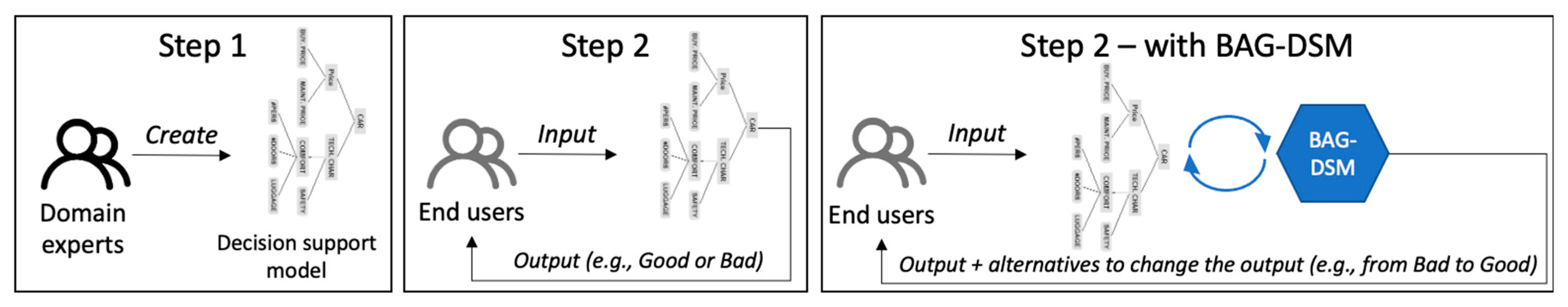
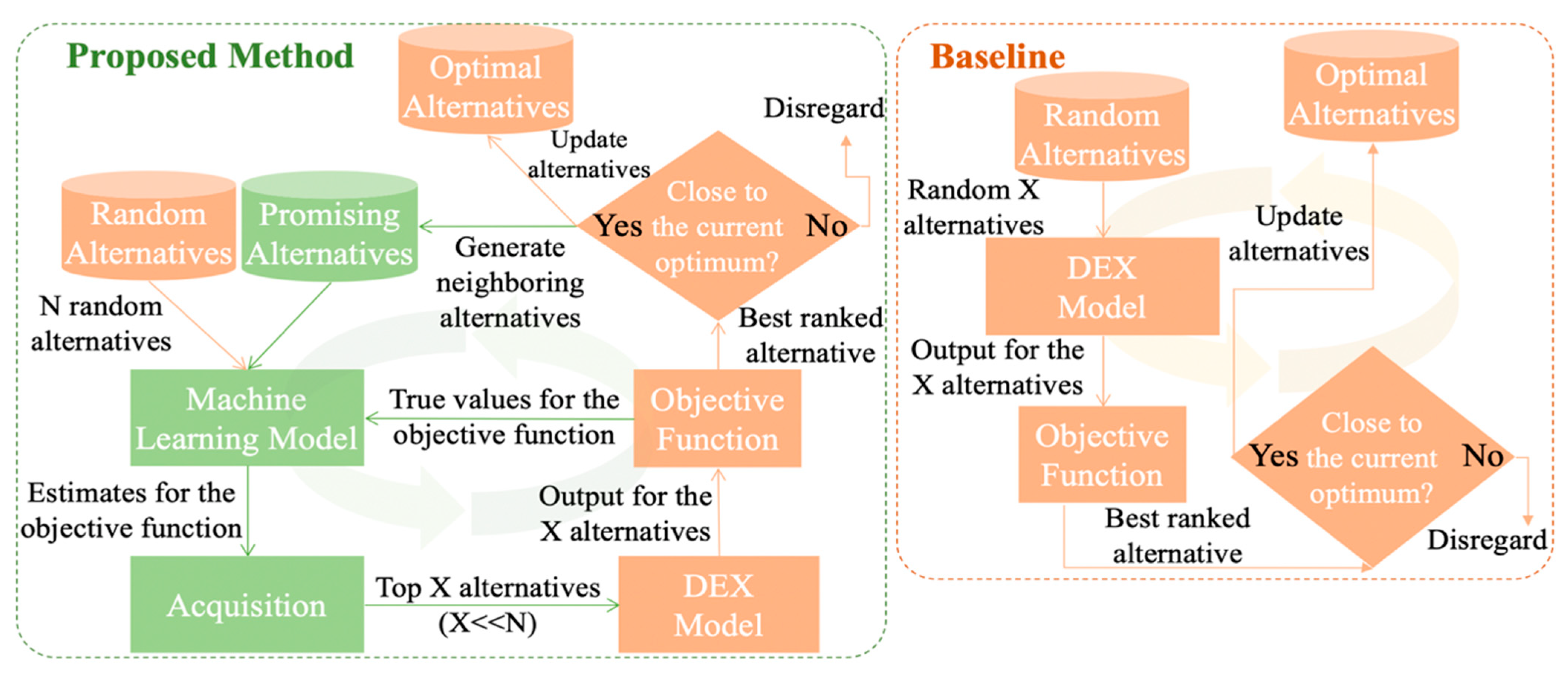
4. Bayesian Alternative Generator for Decision Support Models (BAG-DSM)

An efficient search strategy is required to generate alternatives that require the smallest change in the current alternative to obtain a desirable outcome. A naïve approach would be to generate all possible alternatives or to iteratively generate random alternatives and evaluate the outcome for each alternative (see Figure 7). However, for reasonably complex decision models, the search space can be enormous, rendering the naïve approaches unsuitable.
A more appropriate approach would be to use an informed search based on the history of previously generated and evaluated alternatives. The history can be used to estimate the search space and the behavior of the decision model. Based on that estimation, more promising alternatives can be acquired. By focusing on the more promising alternatives, the search space is reduced, and consequently, the time needed to find the appropriate alternatives is also reduced. Such an informed search is performed stochastically using Bayesian optimization. The proposed method, BAG-DSM, is depicted in Figure 7 and described in the following subsections. BAG-DSM assumes that we do not know the internal rules by which the decision models operate. Thus, it falls into the category of “black-box” optimization techniques. Knowing and utilizing the decision rules might help the search algorithm, but this option was not addressed in this study.

4.1. Problem Formulation

The problem of generating alternatives that require the smallest change in the current alternative to obtain a desirable outcome can be defined as an optimization problem with two objectives: (1) improved outcome (desired output) of the decision model and (2) maximum similarity between the current alternative c ¯ , and the new proposed alternative x ¯ . For each decision model (aggregating function) F , one alternative x ¯ can be defined as a tuple of attributes x ¯ = ( x 1 , x 2 , , x n ) , where each attribute can take any value of a limited set of values. Usually, that set includes preferentially ordered ordinal values (e.g., “low”, “medium”, and “high”), and those values can be encoded with integers (e.g., 0, 1, and 2). Based on that encoding, a distance function d can be defined. The specific distance function used by BAG-DSM is a modified Euclidean distance between the candidate alternative x ¯ and the current alternative c ¯ . This distance considers only the attributes for which the candidate alternative has higher (preferentially better) values compared to the current alternative c ¯ .
d c ¯ , x ¯ = x j c j ,   i f   x j > c j ,   j = 1 , ,   n     0 ,   i f   x j c j ,   j = 1 , ,   n .
From the distance function, a similarity function s can also be defined as one minus the normalized distance. The distance is normalized using the max _ d i s t a n c e , i.e., the maximum plausible distance for the specific problem. For example, if x ¯   has 20 attributes with possible values between 0 and 2, and if each attribute has the highest possible value (2), and if c ¯ has only attributes with the lowest possible value (0), the maximum distance is 20 * 2.
c ¯ , x ¯ , = 1 d c ¯ , x ¯ max _ d i s t a n c e     .
Finally, the objective function can be defined as:
f c ¯ , x ¯ ,   F = s c ¯ , x ¯ , i f   F x ¯ > F c ¯     0 , i f   F x ¯ F c ¯
where F x ¯ is the output of the model for the specific alternative. By optimizing f , the method searches for alternatives that are as similar as possible to c ¯ and improve the output of the decision model ( F x ¯ > F c ¯ ). The definitions of d ,   s , and f are for a scenario where the desired outcome is an improvement of the current alternative ( F x ¯ > F c ¯ ). For the opposite scenario, i.e., if one would like to decrease the output of the decision model, d should be modified to consider only the attributes for which the alternative has lower values compared to the current alternative c ¯ . Additionally, in that scenario, f should be modified to return the similarity when F x < F c ¯ and 0 otherwise. Such a scenario can be used to explore the stability of the current alternative c ¯ .
Bayes’ theorem describes a way of calculating the conditional probability of an event:
P A | B = P ( B | A ) P A P B .
This equation can be simplified by removing the normalizing value of P B and describing the conditional probability as a proportional quantity ( A | B P B | A P A ), where P A | B is the posterior probability, P B | A is the likelihood, and P A is the prior probability (therefore, posterior l i k e l i h o o d   p r i o r ). Following this idea, we can generate specific alternatives and evaluate them using the objective function f . By iteratively generating such alternatives, learning data D can be created: D = x 1 ¯ , f x 1 ¯ ,   x 2 ¯ , f x 2 ¯ , , x k ¯ , f x k ¯ , where x 1 ¯ , x 2 ¯ , …, x k ¯ are k vectors (alternatives), each of them consisting of n attribute values (e.g., x k   ¯ = ( x k 1 ,   x k 2 , ,   x k n ) ), and f x k ¯ is the objective function that returns the outcome for each alternative x k ¯ . These data define the prior probability for the specific problem. The likelihood function is defined as the probability of observing the data given the objective function   f   P D | f . This likelihood function will change as more alternatives are generated:
P f | D = P D | f P f
where P f | D represents the updated expectations about the unknown objective function [27]. This step can also be interpreted as estimating the objective function with a surrogate function.
A surrogate function is a Bayesian approximation of the objective function that can be sampled efficiently. The surrogate function   P f | D provides an estimate of the objective function by summarizing the conditional probability of the objective function f , given the learning data D . Usually, the surrogate function is learned using regression algorithms, with the D representing the input and the objective value (the output of the objective function) representing the output to the model. This is often modeled using a Gaussian process (GP) [28,29,30] because regression models based on the GP do not output just a single predicted value, but rather they output the whole probability distribution. By exploiting the mean and the standard deviation of the output distribution, one can balance the tradeoff of exploiting (higher mean) and exploring (higher standard deviation). In Bayesian optimization, that output distribution also represents the posterior distribution. Since GP models are computationally expensive with the complexity of O ( n 3 ), ensemble models such as random forest (RF) can also be used [26,28,31,32]. In that case, the mean and the variance are calculated based on the predictions of all base models available in the ensemble. BAG-DSM uses RF with 1000 decision trees as base models. The surrogate model ( S M ) is used to estimate the objective value of a large number of candidate alternatives from the search space. From those estimations, one or more candidates can be selected and evaluated with the objective function. The selection process also involves the use of the posterior (the output of the surrogate model) in a function known as the acquisition function.
An acquisition function is a function by which the posterior is used to select the next alternative (sample) from the search space. The acquisition function is used to optimize the conditional probability of locations in the search space that are most likely to generate good alternatives. Example acquisition functions that can be used are: expected improvement [33], predicted improvement [34], and upper confidence bound [35]. The acquisition function operates on top of the mean and standard deviation of the S M ’s output. We tested several acquisition functions, and their influence on the overall performance was minimal. The final version of BAG-DSM uses the expected improvement ( E I ) as an acquisition function:
E I x ¯ , x b = µ S M x ¯ S b ξ   Φ Z + σ S M x ¯ Φ Z ,     i f     σ S M x ¯ > 0 0 , i f σ S M x ¯ = 0
where,
Z = µ S M x ¯ S b ξ / σ S M x ¯ ,     i f       σ S M x ¯ > 0   0 ,       i f       σ S M x ¯ = 0  
where S M x ¯ is the output of all base models in the S M for the alternative x ¯ ; S b   is the maximum predicted value by the S M from all previous observations; Φ (·) is the normal cumulative distribution function, and ξ is a constant that controls the tradeoff between global search and local optimization (exploration/exploitation). In our experiments, we used ξ = 0.01 as proposed by Lizotte [36]. In simpler terms, this acquisition function checks the improvement that each candidate alternative brings with respect to the maximum known value ( µ S M x ¯ x b ) , and scales those improvements with respect to the uncertainty. The uncertainty is calculated empirically from the standard deviation of the predictions of the based models available in the S M . If two alternatives have a similar mean value, the one with higher uncertainty ( σ S M x ¯ will be preferred by the acquisition function.
Finally, we need to define the generator of alternatives. BAG-DSM uses two generators of alternatives: a neighborhood generator and a random generator. Based on the distance function   d , a neighborhood relation can be defined. Two alternatives x 1 ¯ and x 2 ¯ are considered as neighbors with a degree k, if d x 1 ¯ , x 2 ¯ = k. For example, x 1 ¯ and x 2 ¯ are considered neighbors with a degree k = 1, if the distance between x 1 ¯ and x 2 ¯ is 1. They are considered as neighbors with a degree k = 2 if the distance between x 1 ¯ and x 2 ¯ is 2. The distance function d is defined in Equation (3). In scenarios where the desired outcome is an improvement of the current alternative, d calculates how many attributes in x 2 ¯ have a bigger value than the corresponding attributes in x 1 ¯ . In the opposite scenarios, i.e., one would like to decrease the output of the decision model, d calculates how many attributes in x 2 ¯ have a smaller value than the corresponding attributes in x 1 ¯ .
Consequently, for a given alternative x , ¯   we can generate a set of neighbors with degree k, by alternating the value of k different attributes in x ¯ . The degree k was set experimentally. The relation between the computing time and k is exponential and is mostly affected by the number of input attributes. For the models with a depth of 3, we used k = 5; for the models with a depth of 4, we used k = 4; and for models with a depth of 5, we used k = 3.
The random generator is a generator of alternatives that: (1) avoids generating known alternatives; and (2) is conditioned by the best-known (with respect to the objective function) alternative discovered in the previous iterations. That is implemented by disregarding the alternatives that have an optimization score lower than a certain threshold. The threshold was set experimentally to 80% from the best-known optimization score, calculated from the previous iterations.

4.2. Implementation

Algorithm 1 presents the implementation of BAG-DSM. The algorithm returns a set of optimally best (optimal) alternatives. In this set, all the alternatives have an equal score with respect to the objective function. The function check_promising_values runs the S M on a set of promising alternatives. This set contains all alternatives that have been previously generated as neighbors to a specific optimal alternative but have not been evaluated with the D M because the acquisition function has selected other alternatives. This enables one final check of the most promising solutions, which may have been missed because of an earlier bad prediction of the S M . Since the S M is retrained at each iteration, it is expected that its performance improves over time. This step is more computationally expensive as it checks a larger set of candidate alternatives and is performed only once.
Algorithm 1: Input: Decision model F and current alternative CA; Output: best_alternatives
# parameters and initialization
 max_e = 150 # maximum number of epochs
 n_candidates = 10 # number of candidates per iteration
 objective_jitter = 0.8 # if an alternative is close to the current best (e.g, 80% as good as the current best, the alternative’s
neighbors should be checked)
 random_sample_size = 10,000 #number of randomly generated alternatives
 best_alternatives = []
 surrogate_model = new Random_Forest()
 promising_alternatives_pool = []

#initial values
 candidate_alternatives = generate_random_alternatives (10)
 real_objective_values = objective_function (F, CA, alternatives)
 surrogate_model.fit (candidate_alternatives, real_objective_values)
 known_alternatives.add (candidate_alternatives, real_objective_values)
 best_alternative, best_score = max (candidate_alternatives, real_objective_values)
 neighboring_alternatives= generate_neighborhood (best_alternative)
while counter < max_e do:
            If size (neighboring_alternatives) > 0:
              alternatives_pool = neighboring_alternatives
            else:
              alternatives_pool = gen_rand_alternatives (best_alternative, random_sample_size)
            # get top ranked (e.g., 10) candidates using the acquisition function
            candidate_alternatives, candidate_scores = perform_acquisition (alternatives_pool, n_candidates)

            #evaluation of candidate alternatives
            real_objective_values = objective_function (F, CA, alternatives)
            known_alternatives.add (candidate_alternatives, real_objective_values)

            #update current best and promising alternatives
            i = 0
            while i < size (candidate_scores) do:
              if best_score*objective_jitter <= candidate_scores[i] do:
                  neighboring_alternatives = generate_ neighbourhood (candidate_alternatives[i])
                  promising_alternatives_pool.add (neighboring_alternatives)
              if  best_score < candidate_scores[i] do:
                  best_alternatives = []
                  best_alternatives.add (candidate_alternatives[i])

              if  best_score==candidate_scores[i] do:
                  best_alternatives.add (candidate_alternatives[i])
              i++
            #update the surrogate model
            surrogate_model.fit (candidate_alternatives, real_objective_values)
            counter++
end

#peform final check of the promising alternatives
 best_alternatives = check_promising_values(promising_alternatives_pool,best_alternatives)
return best_alternatives

5. Experiments

5.1. Experimental Setup

BAG-DSM was evaluated with 43 decision models: the real-life model depicted in Figure 5, and the 42 benchmark models summarized in Table 1. The real-life model demonstrates the utility of BAG-DSM in a real-life scenario. With this model, 23 different randomly sampled alternatives were used as starting alternatives and for each alternative, and BAG-DSM was run to find a set of optimal solutions.
On the other hand, the 42 benchmark models allowed for a detailed analysis of BAG-DSM’s performance under a variety of circumstances. For each benchmark model, nine different randomly sampled starting alternatives (current alternatives   c ¯ ) were sampled. Three of those alternatives had a final attribute value of “low”, three had a final attribute value of “medium”, and three had a final attribute value of “high”. For each current alternative, BAG-DSM generates new alternatives that require the smallest change in the current alternative to obtain a desirable outcome. The desirable outcome was also varied:
  • starting with output attribute value “low”, generate alternatives that would improve the final attribute value to “medium” (positive change),
  • starting with output attribute value “low”, generate alternatives that would improve the final attribute value to “high” (positive change),
  • starting with output attribute value ‘medium’, generate alternatives that would improve the final attribute value to ‘high (positive change),
  • starting with output attribute value “medium”, generate alternatives that would change the final attribute value to “low” (negative change),
  • starting with output attribute value “high”, generate alternatives that would change the final attribute value to “medium” (negative change),
  • starting with output attribute value “high”, generate alternatives that would change the final attribute value to “low” (negative change).
Each experiment ran for a minimum of 100 epochs, a maximum of 150 epochs, and was terminated after 50 epochs without improvement (i.e., a better alternative was not discovered compared to the current best). The experiments were performed on a server with Intel(R) Xeon(R) CPU E5-2680 v3 @ 2.50 GHz and 150 GB RAM. Each experiment was repeated 10 times to minimize the influence of the randomized steps on the experimental results. BAG-DSM and the experiments were implemented in Python and are available online (https://repo.ijs.si/martingjoreski/bag-dsm accessed on 5 May 2022).
All experiments were performed both for the proposed BAG-DSM and for the baseline method (also depicted in Figure 7), i.e., a method that iteratively evaluates random alternatives and, at each iteration, saves only the alternatives that are equally good or better than the previous best-ranked alternative. To provide a fair comparison, the random alternatives were generated by the same random generator used by BAG-DSM.
Additionally, for each experimental run, the baseline method was given an equal amount of execution time as the BAG-DSM. For example, if the BAG-DSM finished an experiment in 5 min with a certain setup, the baseline method was given 5 min to perform a random search for the same experimental setup. The comparisons of performances undergo statistical analysis of differences in achieved performances by both methods. For that purpose, the Shapiro–Wilk test is used for testing the normality of performance distributions, the Kruskal test is used for testing the homoscedasticity, and the Mann–Whitney U test for testing the significance of differences.
The evaluation metrics used for comparison with the baseline are:
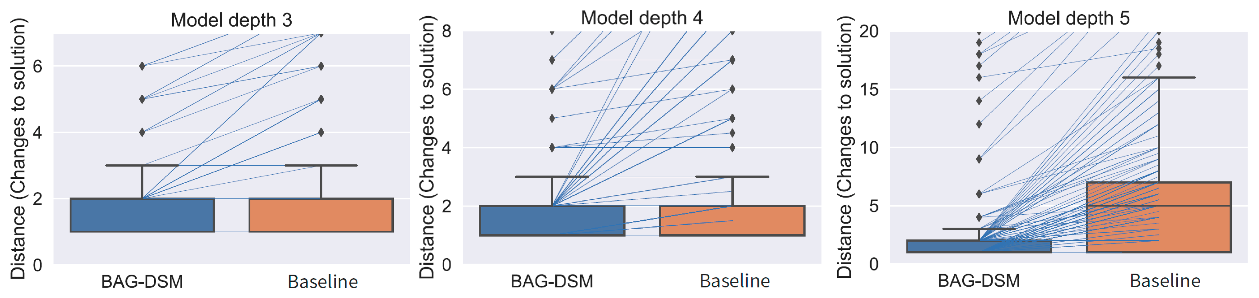
  • distance—as defined in Equation (3). The shorter the distance is, the better the solutions are;
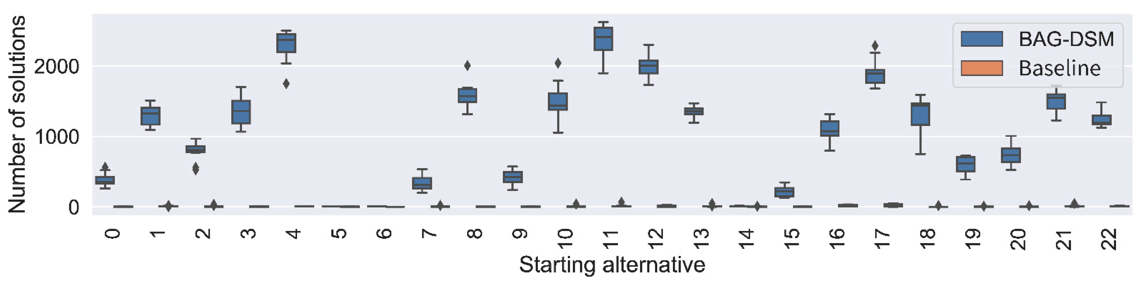
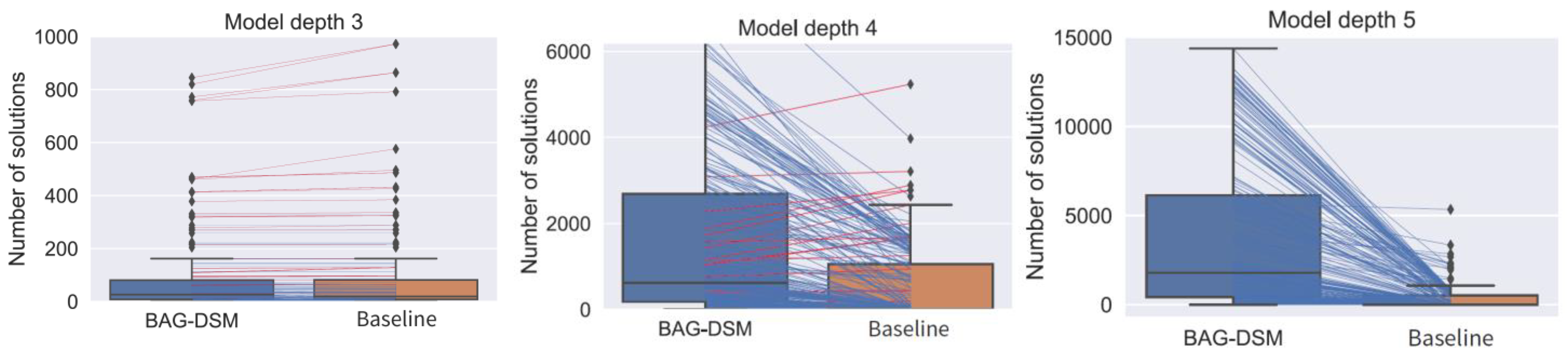
  • optimal solution set size—the method outputs a set of optimal alternatives that have an equal score with respect to the objective function (defined in Equation (5)). The bigger the solution set is, the more options to choose from for the user;
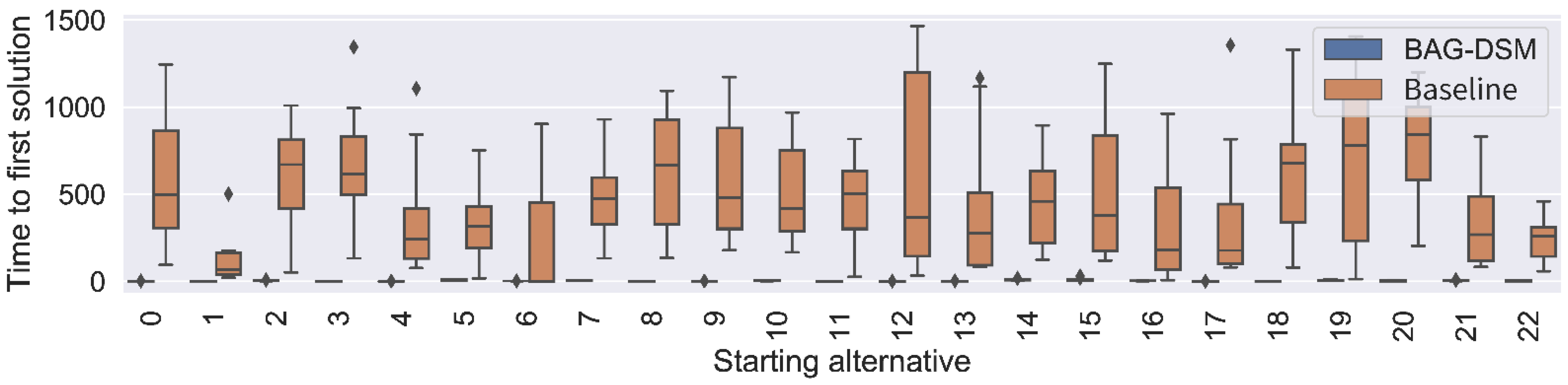
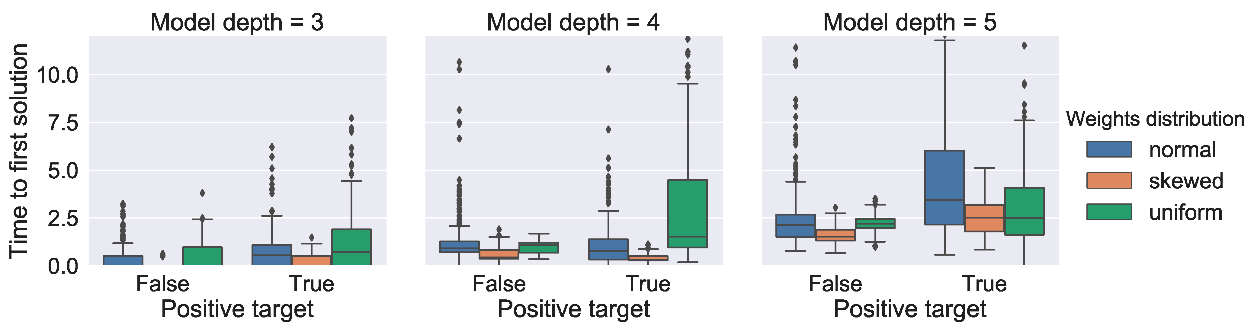
  • time to first optimal solution—i.e., the time required to generate the first solution in the optimal solution set.

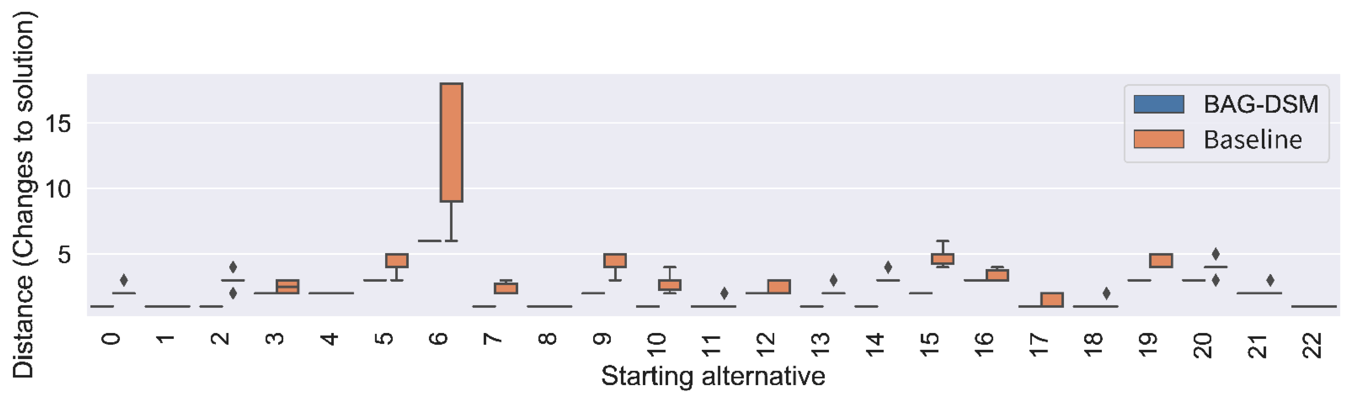
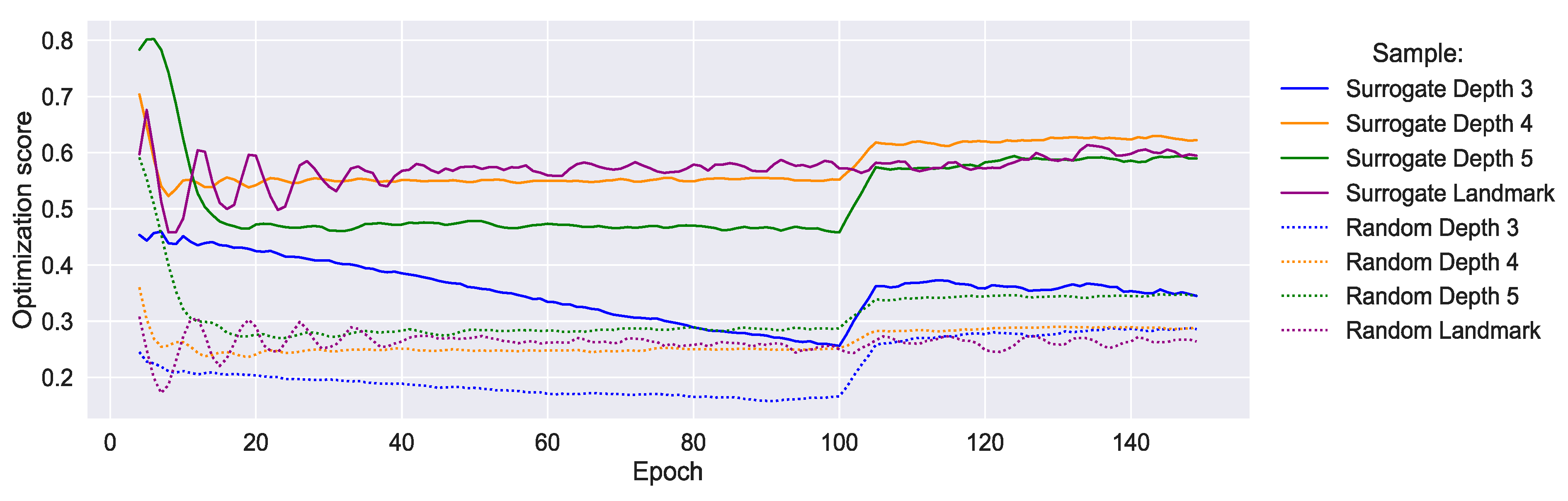
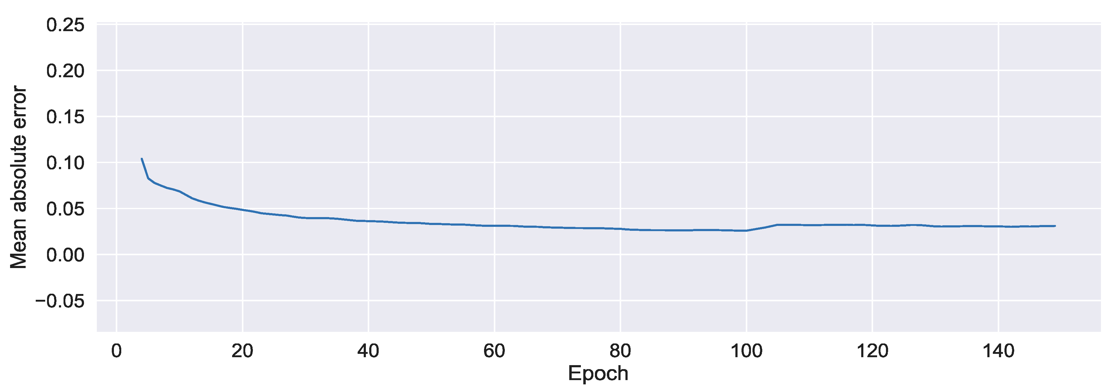
5.2. Experimental Results

The next two subsections present a comparison of the BAG-DSM with the baseline method on the real-life model and a comparison of BAG-DSM with the baseline method on the benchmark models.

5.2.1. Landmark Use Case

The most important metric that presents the quality of the solutions generated by BAG-DSM is the distance, i.e., the number of attribute changes required to achieve the final solution starting from the current state of the current alternative (as defined in Equation (3)). Figure 8 presents the distance required to achieve the final solution with the real-life model. On the x axis are the 23 randomly generated starting alternatives. The boxplots were generated using the results from the 10 repetitions for each experiment. Several observations can be seen from this figure: (i) the boxplots for BAG-DSM are always just a horizontal line, meaning that BAG-DSM was stable and it always found solutions with the same quality, i.e., same distance; (ii) the results of BAG-DSM are equally good as the results of the baseline method, and in the majority of the cases even better; (iii) in all of the cases, the final solution found by BAG-DSM was at a distance shorter than 5, i.e., only 5 (or fewer) attributes out of 26 need to be changed to reach the required optimal alternative.
For each input starting alternative, the method outputs a set of optimal alternatives that have an equal distance to the starting alternative with respect to the objective function (defined in Equation (5)). The bigger the solution set is, the more options to choose from for the user. Figure 9 presents the size of the solution sets for each of the 23 alternatives. It can be seen that BAG-DSM found larger solution sets than the baseline in most of the cases.
Figure 9 shows that the final output of the algorithm can consist of thousands of different alternatives. However, from a user perspective, only a few alternatives should be enough. For that reason, the time required to generate the first solution is a relevant metric to consider. Figure 10 presents the time (in seconds) required to generate the first solution for each of the 23 alternatives. From the results, it can be seen that BAG-DSM was faster than the baseline in all of the cases, with a difference of close to 500 s on average. One more important consideration is that the standard deviation of the boxplots for BAG-DSM is much smaller than the baseline’s standard deviation, which means that BAG-DSM is also stable with respect to the time required to generate the first solution.
BAG-DSM’s dominance has been confirmed with statistical tests of significance. Considering both performance measures (time to first solution and number of solutions), BAG-DSM stochastically dominates the baseline method (p-value close to 0)—for more details, please check Supplementary Materials, Section S2.2.

5.2.2. Benchmark Models

The same experiments presented in the previous subsection were repeated for the 42 benchmark models, and the same metrics were used to analyze the results. Thus, the next three figures present the distances, time to the first solution, and the number of solutions. Different from the previous graphs, the results are presented via paired boxplots. All our experiments are paired experiments, i.e., for given experimental conditions (e.g., a decision model, a starting alternative, and a desired outcome), a pair of experiments was performed, one set of experiments with the proposed method and another set of experiments with the baseline. We use the term “set of experiments” because each experiment was repeated 10 times to minimize the influence of the randomized steps on the experimental results. The lines connect the experimental runs that had the same experimental conditions (same model and same starting alternative). The blue line shows that our method was better for those specific experimental conditions. The red line shows that the baseline was better for those specific experimental conditions. The corresponding set of alternatives is compared using: the number of attribute changes required to reach the generated alternatives (Figure 11); the time to obtain the first appropriate alternative, Figure 12; and the number of generated alternatives (Figure 13).
Figure 11 presents the distance between the final solution and the starting alternative. From the results, it can be seen that in all of these experiments, BAG-DSM found solutions with equal or shorter distances compared to the solutions found by the baseline. The difference is larger for the more complex models (depth 4 and depth 5).
Figure 12 presents the time (in seconds) required to find a first solution. The blue horizontal line represents the experimental runs where BAG-DSM found the first solution faster than the baseline. Red horizontal lines represent the experimental runs where the baseline method was faster. From the results, it can be seen that for the more complex models (depth 4 and depth 5), BAG-DSM was much faster by finding the first solutions in the first few seconds, while the baseline method required more than 100 s in some of the cases. The only experiments in which the baseline performed better than BAG-DSM were those for the models with depth 3. However, the difference is smaller than 3 s.
The observations have been statistically confirmed with statistical tests. BAG-DSM significantly dominates the baseline across all models (p-value very close to 0), as well as with respect to individual model types (e.g., models with normal, skewed, or uniform distribution or various depths). However, BAG-DSM has a less significant dominance in the problems with uniform distribution of attributes’ weights compared to the other two (Supplementary Materials—Section S2.1.1).
Figure 13 presents the size of the solution set (bigger is better) generated by the two methods. From the results, it can be seen that for the more complex models (depth 4 and depth 5), BAG-DSM found many more solutions than the baseline. There were some cases where the baseline found larger solution sets, especially for the models with depth 3. However, it should be noted that here we compare only the size of the solution set and not the quality of the solution sets. This means that the baseline approach might have found 100 solutions with a distance of 5, i.e., require 5 attribute changes, compared to BAG-DSM with 10 solutions with a distance of 3. Figure 11 already showed that the quality of the solutions generated by the Bayesian is better than those generated by the baseline in the majority of the cases.
Statistical tests have been performed for equally distant solutions found by both methods, and similar findings, as above, are confirmed (Supplementary Materials—Section S2.1.2). Namely, an overall significant stochastic dominance is observed, while such dominance is lacking over models with uniformly distributed weights (p-value is 0.07) and models with a depth of 3 (p-value is 0.6).

5.2.3. Performance Analysis

The experimental results from the previous subsections showed that BAG_DSM outperformed the baseline in all of the experiments. The following results present how the method’s performance depends on the complexity of the decision model, which was expressed through the depth of the decision model and the distribution attributes’ weights (attributes’ importance).
Figure 14 presents the time (in seconds) required to find a first solution of the final set of solutions for the benchmark models. The overall median of the time to the first solution is 1.67 s. Additionally, the figure contains three sets of boxplots (depth 3, depth 4, and depth 5), where the boxplots are color-coded with respect to the distribution of the attributes’ weights. The x-axis presents the direction of the search. For example, the search direction would be positive (positive target) if the starting alternative has an output attribute value of “medium”, and the method generates alternatives that would improve the final attribute value to “high”. On the other hand, the search direction would be negative if the starting alternative has an output attribute value of “medium”, and the method generates alternatives that would decrease the final attribute value to “low”. From the figure, it can be noticed that the time to the first solution increases as the depth of the models increases. However, even though the depth of the model is a parameter that increases the search exponentially, the increase in time (seconds) is rather linear, which is an experimental proof of the method’s scalability. Additionally, from the figure, it can be seen that the decision models with a skewed distribution of the attributes’ weights require the smallest amount of time to find the first solution. Regarding the direction of the search (positive vs. negative target), it seems that BAG-DSM finds first solutions faster when the direction is negative. This is probably because the size of the solution set is bigger when the direction is negative, i.e., it is easier to decrease the value of the output attribute (e.g., from “medium” to “low”), than to increase it (e.g., from “medium” to “high”).
In each epoch, BAG-DSM selects the top 10 alternatives ranked by the estimated optimization score. The higher the score, the better the alternatives are. The selected alternatives depend on the acquisition function, which in turn depends on the predictions of the surrogate model. Figure 15 presents the average optimization score in each epoch for the four different model types: benchmark model with a depth of 3, benchmark model with a depth of 4, benchmark model with a depth of 5, and the real-life model (Landmark). For comparison, the average optimization score of 10 randomly sampled alternatives at each epoch is also presented (dashed line). From the figures, it can be seen that the optimization score of the random samples is significantly lower than the optimization score of the samples selected using the surrogate model. Additionally, it can be seen that the optimization score stays high throughout all the epochs. This indicates that the generator of alternatives generates good candidates, and BAG-DSM discovers new alternatives continuously.
In addition, for some of the experiments, the algorithm stopped after 100 epochs because there was no improvement in the last 50 learning epochs. This can be noticed as a sudden increase in the average optimization score in the figure. That is because the average of the first 100 epochs is calculated over all the experimental runs, and the average of the last 50 epochs is calculated over a smaller number of experimental runs, i.e., those that did not finish in the first 100 epochs.
Figure 16 presents the average mean absolute error (MAE) of the surrogate model, i.e., estimated optimization score calculated using the surrogate model vs. true optimization score calculated using the objective function. The shaded part presents one standard deviation in each direction. It can be noticed that the MAE gradually decreases. This is because, at each epoch, the training dataset for the surrogate model increases, and the surrogate model improves after each retraining. In addition to the MAE, the standard deviation of the MAE also decreases, showing that the stability of the surrogate models also improves over time.
In summary, these results indicate that: (i) BAG-DSM is suitable for the task—on average, it generates at least one appropriate alternative within two seconds (Figure 14); (ii) BAG-DSM is scalable—the relation between the depth of the multi-attribute hierarchical models (a parameter which increases the search space exponentially) and the time to obtaining the first appropriate alternative was linear and not exponential (Figure 14); (iii) BAG-DSM’s generator of alternatives generates good alternatives (better than random sampling) and BAG-DSM discovers good alternatives continuously (Figure 15); (iv) the BAG-DSM surrogate model (random forest, RF) is appropriate for the task—RF’s MAE and standard deviation of the MAE decrease at each epoch (Figure 16).

6. Discussion

6.1. Results Discussion

The experimental results showed that BAG-DSM outperformed the baseline in all of the experiments. However, a close examination of the performances of the methods per characteristic of the solution and search spaces (and their ratio), i.e., the complexity of the decision models, is necessary in order to understand the situation where one or another method is more suitable. For that purpose, we investigated how BAG-DSM’s performance depends on the depth of the decision model and the distribution of the attribute weights (attributes’ importance).
As observed through the empirical and statistical analysis, BAG-DSM significantly outperforms the baseline method with respect to the time needed to find the first optimal alternative, and this is particularly true for the larger models represented with normal and skewed distributions of the attributes’ weights. The dominance is less significant with the models with uniformly distributed weights. Such behavior can be explained by the size of the solution space (i.e., the set of possible solutions) and its ratio to the overall search space, which is largest for the uniformly distributed weights, and smallest in the case of skewed distributions of the models’ weights. Similarly, methods with the shallower models tend to have comparable performance in terms of the time to first solution (Supplementary Materials—Section S2.1.1).
The complexity of the decision models, in terms of size and dimensionality of the search space, affects the size of the generated (optimal) solution set. Namely, overall, BAG-DSM significantly outperforms the baseline method, but less significance is observed for models with uniformly distributed weights and models with a depth of 3. The former is explained by the solution-to-search space ratio, which is largest in the case of uniformly distributed weights, and the fact that with the given number of iterations, the baseline can find many options/solutions. This is particularly true for models of depth 3 that are characterized by relatively small alternative spaces, and hence, with those models, both methods achieve comparable results.

6.2. Limitations and Future Work

One assumption in all experiments was that all attributes could be changed. In reality, this is not always true. For example, if we had a decision model for assessing soil quality, the type of the soil at a given location cannot be changed. In the future, this condition can be easily addressed by providing as input only the attributes that can be changed. Additionally, the method implementation is restricted to preferentially ordered ordinal attributes. However, there is a possibility of considering other types of distance measures that would work in nominal settings (e.g., Levenshtein distance).
BAG-DSM is a “black-box” method; given a decision support model, BAG-DSM considers only its input and output attributes but is oblivious to its internal structure. This is both an advantage and a limitation. As an advantage, BAG-DSM is not limited to DEX models but can, in principle, work with any qualitative models that employ preferentially ordered ordinal attributes. As a limitation, BAG-DSM does not use information about internal attribute structure and decision rules; employing this information might considerably reduce the search space but also restrict the method to DEX models only.
Regarding future work, BAG-DSM is stochastic, and the optimality of the final solution cannot be guaranteed. In order to do that, BAG-DSM needs to be additionally validated. Promising options include a comparison of BAG-DSM with deterministic methods and methods that utilize internal rules by which the decision models operate. Finally, BAG-DSM could also be validated on real decision models in order to examine the validity of the output solutions.

6.3. Implications

A typical use case of the proposed method can be presented via the decision support model depicted in Figure 5. The model has 26 input attributes and, consequently, a huge input space (1.59 × 10¹²). Using this model, the end users for whom this model was initially developed can evaluate the primary productivity of their agricultural fields. In scenarios where the output of the model is, for example, “low productivity”, a natural question would be, “What can I do to improve the productivity of my field?”. BAG-DSM answers that question by providing alternatives that lead to the improvement of primary productivity. In another scenario where the output of the model is “high productivity”, a possible question could be, “What can go wrong and degrade the productivity of my field?”. This question is also answered by BAG-DSM by providing alternatives that lead to decreased productivity. The answers are, according to our experiments, of good quality and provided in a short time.
This study demonstrated that BAG-DSM is model agnostic, i.e., it is a general method that works with any DEX decision support model. Furthermore, the mathematical and theoretical background presented in this paper should enable the application of BAG-DSM to any other decision support models using qualitative inputs and outputs. Furthermore, the same approach can be used for generating counterfactual explanations for machine learning models.
Thus, we envision BAG-DSM being used as a plug-in for future decision support models where the end users would receive, besides the output of the decision support models, a list of alternatives that require a minimal number of changes in the input space and yet would cause a change in the output of the decision support model.

7. Conclusions

We presented BAG-DSM, a method for generating alternatives for multi-attribute DEX decision models based on Bayesian optimization. The main goal of BAG-DSM was to generate alternatives that require the smallest change in the current alternative to obtain a desirable outcome. BAG-DSM was extensively evaluated on 42 different benchmark models and one real-life model. The benchmark models were of variable complexity, i.e., variable depth and variable attribute weight distributions. BAG-DSM’s behavior was analyzed with respect to several characteristics: time to find the first appropriate alternative, the number of generated (appropriate) alternatives, and the number of attribute changes required to reach the generated alternatives.
The experimental results confirmed that BAG-DSM is suitable for the task, i.e., it generates at least one appropriate alternative in less than a minute, even for the most complex decision models. In the majority of the cases, the computing time was shorter than that. The discovery of alternatives was equally distributed throughout the overall runtime. An exception to this is the final check performed by the algorithm (see check_promising_values in Algorithm 1), which generates the majority of the alternatives for the more complex models (depth 4 and depth 5). The quality of the alternatives was also appropriate, as in the majority of the cases. The generated alternatives could be reached by fewer than five attribute changes. Finally, the relation between the decision model’s depth and the computing time in the experiments was linear and not exponential, which implies that BAG-DSM is scalable.

Supplementary Materials

The following supporting information can be downloaded at: https://www.mdpi.com/article/10.3390/a15060197/s1.

Author Contributions

Conceptualization, M.G., V.K. and M.B; methodology, M.G., V.K. and M.B.; software, M.G., V.K. and M.B.; validation, M.G. and V.K.; formal analysis, M.G., V.K. and M.B.; investigation, M.G.; resources, M.G., V.K. and M.B.; data curation, M.G. and V.K.; writing—original draft preparation, M.G., V.K. and M.B.; writing—review and editing, M.G., V.K. and M.B.; visualization, M.G., V.K. and M.B.; supervision, V.K. and M.B.; project administration, M.B.; funding acquisition, M.B. All authors have read and agreed to the published version of the manuscript.

Funding

This work was partially funded by the Slovenian Research Agency (ARRS) under research core funding Knowledge Technologies No. P2-0103 (B), and by the Slovenian Ministry of Education, Science and Sport (funding agreement No. C3330-17-529020).

Institutional Review Board Statement

Not applicable.

Informed Consent Statement

Not applicable.

Data Availability Statement

Conflicts of Interest

The authors declare no conflict of interest.

References

  1. Power, D.J. Decision Support Systems: Concepts and Resources for Managers; Quorum Books: Westport, CT, USA, 2002. [Google Scholar]
  2. Turban, E.; Aronson, J.E.; Liang, T.-P. Decision Support Systems and Intelligent Systems; Prentice-Hall: Hoboken, NJ, USA, 2005. [Google Scholar]
  3. Mallach, E. Decision Support and Data Warehouse Systems; Irwin Profesional Publishing: Burr Ridge, IL, USA, 2000. [Google Scholar]
  4. Sadok, W.; Angevin, F.; Bergez, J.-É.; Bockstaller, C.; Colomb, B.; Guichard, L.; Reau, R.; Doré, T. Ex ante assessment of the sustainability of alternative cropping systems: Implications for using multi-criteria decision-aid methods. A review. Agron. Sustain. Dev. 2008, 28, 163–174. [Google Scholar] [CrossRef] [Green Version]
  5. Sadok, W.; Angevin, F.; Bergez, J.-É.; Bockstaller, C.; Colomb, B.; Guichard, L.; Reau, R.; Messean, A.; Doré, T. MASC, a qual-itative multi-attribute decision model for ex ante assessment of the sustainability of cropping systems. Agron. Sustain. Dev. 2009, 29, 447–461. [Google Scholar] [CrossRef] [Green Version]
  6. Martel, J.-M.; Matarazzo, B. Multiple Criteria Decision Analysis: State of the Art Surveys; Springer: New York, NY, USA, 2016. [Google Scholar]
  7. Dogliotti, S.; Rossing, W.; van Ittersum, M. Systematic design and evaluation of crop rotations enhancing soil conservation, soil fertility and farm income: A case study for vegetable farms in South Uruguay. Agric. Syst. 2004, 80, 277–302. [Google Scholar] [CrossRef]
  8. Bohanec, M. DEX (Decision EXpert): A Qualitative Hierarchical Multi-Criteria Method; Kulkarni, A.J., Ed.; Multiple Criteria Decision Making, Studies in Systems, Decision and Control 407; Springer: Singapore, 2022. [Google Scholar]
  9. Kontić, B.; Bohanec, M.; Kontić, D.; Trdin, N.; Matko, M. Improving appraisal of sustainability of energy options—A view from Slovenia. Energy Policy 2016, 90, 154–171. [Google Scholar] [CrossRef]
  10. Erdogan, G.; Refsdal, A. A Method for Developing Qualitative Security Risk Assessment Algorithms. In Risks and Security of Internet and Systems; Springer International Publishing: Dinard, France, 2018; pp. 244–259. [Google Scholar]
  11. Prevolšek, B.; Maksimović, A.; Puška, A.; Pažek, K.; Žibert, M.; Rozman, Č. Sustainable Development of Ethno-Villages in Bosnia and Herzegovina—A Multi Criteria Assessment. Sustainability 2020, 12, 1399. [Google Scholar] [CrossRef] [Green Version]
  12. Bampa, F.; O’Sullivan, L.; Madena, K.; Sanden, T.; Spiegel, H.; Henriksen, C.B.; Ghaley, B.B.; Jones, A.; Staes, J.; Sturel, S.; et al. Harvesting European knowledge on soil functions and land manage-ment using multi-criteria decision analysis. Soil Use Manag. 2019, 35, 6–20. [Google Scholar] [CrossRef] [Green Version]
  13. Lotfi, F.H.; Rostamy-Malkhalifeh, M.; Aghayi, N.; Beigi, Z.G.; Gholami, K. An improved method for ranking alternatives in multiple criteria decision analysis. Appl. Math. Model. 2013, 37, 25–33. [Google Scholar] [CrossRef] [Green Version]
  14. Contreras, I. A DEA-inspired procedure for the aggregation of preferences. Expert Syst. Appl. 2011, 38, 564–570. [Google Scholar] [CrossRef]
  15. Bergez, J.-E. Using a genetic algorithm to define worst-best and best-worst options of a DEXi-type model: Application to the MASC model of cropping-system sustainability. Comput. Electron. Agric. 2012, 90, 93–98. [Google Scholar] [CrossRef]
  16. Wachter, S.; Mittelstadt, B.; Russell, C. Counterfactual Explanations Without Opening The Black Box: Automated Decisions And The Gdpr. Harv. J. Law Technol. 2018, 31, 842–887. [Google Scholar] [CrossRef] [Green Version]
  17. Rudin, C. Stop explaining black box machine learning models for high stakes decisions and use interpretable models instead. Nat. Mach. Intell. 2019, 1, 206–215. [Google Scholar] [CrossRef] [PubMed] [Green Version]
  18. Joshi, S.; Koyejo, O.; Vijitbenjaronk, W.; Kim, B.; Ghosh, J. Towards Realistic Individual Recourse and Actionable Explanations in Black-Box Decision Making Systems. 24 July 2019. Available online: https://arxiv.org/abs/1907.09615 (accessed on 4 May 2022).
  19. Karimi, A.-H.; Barthe, G.; Balle, B.; Valera, I. Model-Agnostic Counterfactual Explanations for Consequential Decisions. 27 May 2019. Available online: https://arxiv.org/abs/1905.11190 (accessed on 4 May 2022).
  20. Wexler, J.; Pushkarna, M.; Bolukbasi, T.; Wattenberg, M.; Viegas, F.; Wilson, J. The What-If Tool: Interactive Probing of Machine Learning Models. IEEE Trans. Vis. Comput. Graph. 2019, 26, 56–65. [Google Scholar] [CrossRef] [PubMed] [Green Version]
  21. Tolomei, G.; Silvestri, F.; Haines, A.; Lalmas, M. Interpretable Predictions of Tree-based Ensembles via Actionable Feature Tweaking. 20 June 2017. Available online: https://arxiv.org/abs/1706.06691 (accessed on 4 May 2022).
  22. Ustun, B.; Spangher, A.; Liu, Y. Actionable Recourse in Linear Classification. In Proceedings of the Conference on Fairness, Accountability, and Transparency, Atlanta, GA, USA, 29–31 January 2019; pp. 10–19. [Google Scholar] [CrossRef] [Green Version]
  23. Roy, B. The Optimisation Problem Formulation: Criticism and Overstepping. J. Oper. Res. Soc. 1981, 32, 427. [Google Scholar] [CrossRef]
  24. Sanden, T.; Trajanov, A.; Spiegel, H.; Kuzmanovski, V.; Saby, N.P.A.; Picaud, C.; Henriksen, C.B.; Debeljak, M. Development of an Agricultural Primary Productivity Decision Support Model: A Case Study in France. Front. Environ. Sci. 2019, 58. [Google Scholar] [CrossRef] [Green Version]
  25. Kuzmanovski, V.; Trajanov, A.; Džeroski, S.; Debeljak, M. Cascading constructive heuristic for optimization problems over hierarchically decomposed qualitative decision space. 2021; submitted. [Google Scholar]
  26. Rezende, D.J.; Mohamed, S.; Wierstra, D. Stochastic Back-Propagation and Variational Inference in Deep Latent Gaussian Models. 16 January 2014. Available online: https://citeseerx.ist.psu.edu/viewdoc/download?doi=10.1.1.753.7469&rep=rep1&type=pdf (accessed on 4 May 2022).
  27. Brochu, E.; Cora, V.M.; de Freitas, N. A Tutorial on Bayesian Optimization of Expensive Cost Functions, with Application to Active User Modeling and Hierarchical Reinforcement Learning. 14 December 2010. Available online: https://arxiv.org/abs/1012.2599 (accessed on 4 May 2022).
  28. Snoek, J.; Rippel, O.; Swersky, K.; Kiros, R.; Satish, N.; Sundaram, N.; Patwary, M.; Prabhat, M.; Adams, R. Scalable Bayesian Optimization Using Deep Neural Networks. In Proceedings of the International Conference on Machine Learning, Lille, France, 6–11 July 2015. [Google Scholar]
  29. de Freitas, J.F.G. Bayesian Methods for Neural Networks. Ph.D. Thesis, University of Cambridge, Cambridge, UK, 2003. [Google Scholar]
  30. Hutter, F.; Hoos, H.H.; Leyton-Brown, K. Sequential Model-Based Optimization for General Algorithm Configuration. In International Conference on Learning and Intelligent Optimization; Springer: Berlin/Heidelberg, Germany, 2011; pp. 507–523. [Google Scholar]
  31. Rasmussen, C.E.; Williams, C.K.I. Gaussian Processes for Machine Learning; MIT Press: Cambridge, MA, USA, 2006. [Google Scholar]
  32. Hutter, F.; Hoos, H.H.; Leyton-Brown, K. Sequential Model-Based Optimization for General Algorithm Configuration (Extended Version); Technical Report TR-2010–10; University of British Columbia, Computer Science: Endowment Lands, BC, Canada, 2010. [Google Scholar]
  33. Močkus, J. On bayesian methods for seeking the extremum. In Proceedings of the IFIP Technical Conference on Optimization Techniques, Novosibirsk, Ruassia, 1–7 July 1974. [Google Scholar]
  34. Kushner, H.J. A New Method of Locating the Maximum Point of an Arbitrary Multipeak Curve in the Presence of Noise. J. Basic Eng. 1964, 86, 97–106. [Google Scholar] [CrossRef]
  35. Srinivas, N.; Krause, A.; Kakade, S.; Seeger, M. Gaussian process optimization in the bandit setting: No regret and exper-imental design. In Proceedings of the International Conference on Machine Learning, Haifa, Israel, 21–24 June 2010. [Google Scholar]
  36. Lizotte, D.J. Practical Bayesian Optimization. Ph.D. Thesis, University of Albert, Edmonton, AB, Canada, 2008. [Google Scholar]
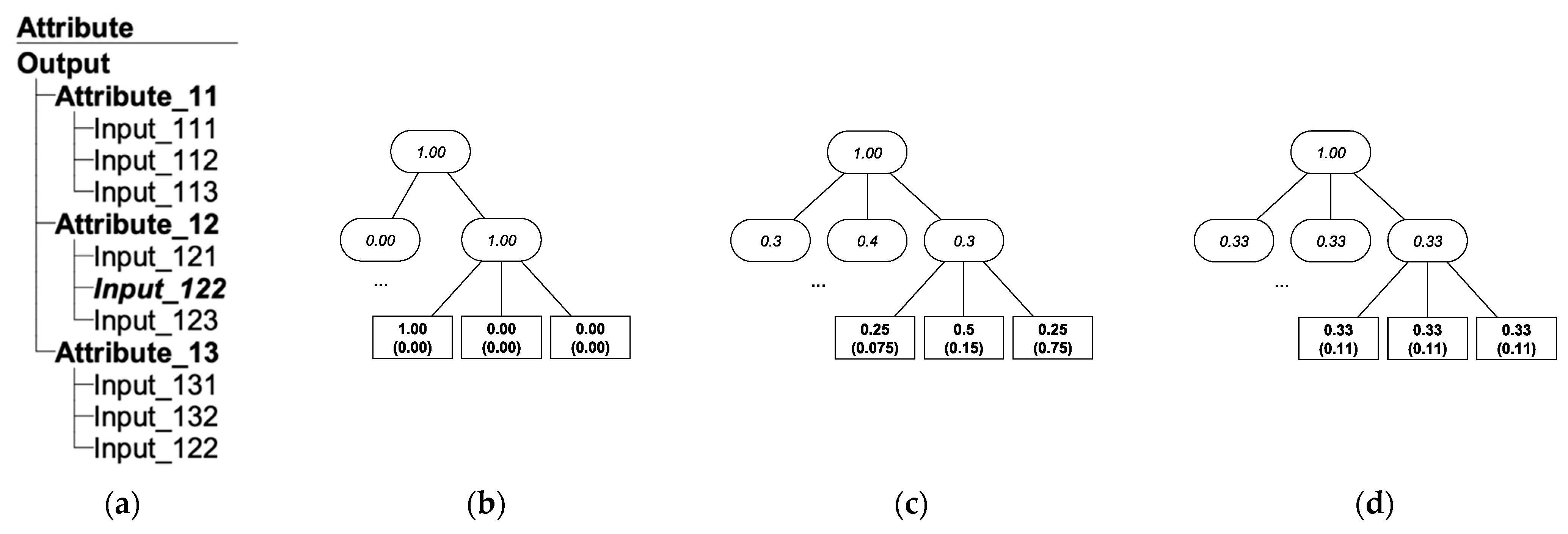
Figure 1. Differences between a typical usage of decision support models (Step 1 and Step 2) and augmented usage with BAG-DSM (Step 1 and Step 2—with BAG-DSM).
Algorithms 15 00197 g001
Figure 2. Structure and value scales of a DEX decision model for the evaluation of vehicles [8].
Algorithms 15 00197 g002
Figure 3. Decision rules for aggregating PRICE and TECH.CHAR. to CAR.
Algorithms 15 00197 g003
Figure 4. Example evaluation of two cars.
Algorithms 15 00197 g004
Figure 5. Structure of a DEX decision model for the assessment of primary productivity of agricultural fields [24].
Algorithms 15 00197 g005
Figure 6. Examples of the structure and weight distributions of a benchmark DEX decision model. (a) The hierarchical structure of a benchmark DEX model with a depth of 3 levels and one linked attribute (Input_122); (bd) examples of skewed (b), normal (c), and uniform (d) distributions of aggregation weights [26].
Algorithms 15 00197 g006
Figure 7. Proposed BAG-DSM method for generating alternatives (left) vs. naïve approach (right).
Algorithms 15 00197 g007
Figure 8. Boxplots for the distances (shorter is better) between the current alternative and the optimal alternative found by BAG-DSM (Bayesian) vs. baseline for the Landmark model.
Algorithms 15 00197 g008
Figure 9. Boxplots for the size of the solution set (bigger is better) generated by BAG-DSM vs. baseline for the Landmark model.
Algorithms 15 00197 g009
Figure 10. Boxplots for the time (shorter is better) required to find the first optimal alternative by BAG-DSM vs. baseline for the Landmark model.
Algorithms 15 00197 g010
Figure 11. Paired boxplots for the distances (shorter is better) between the current alternative and the optimal alternative found by BAG-DSM (Bayesian) vs. baseline for decision support models with a depth of 3, 4, and 5. The horizontal lines connect two experimental runs with the same experimental setup.
Algorithms 15 00197 g011
Figure 12. Paired boxplots for the time (shorter is better) required to find the first optimal alternative by BAG-DSM vs. baseline for decision support models with a depth of 3, 4, and 5. The horizontal lines connect two experimental runs with the same experimental setup. The red lines represent the experimental setups in which the baseline performed better.
Algorithms 15 00197 g012
Figure 13. Paired boxplots for the size of the solution set (bigger is better) generated by BAG-DSM vs. baseline for decision support models with a depth of 3, 4, and 5. The horizontal lines connect two experimental runs with the same experimental setup. The red horizontal lines represent the experimental setups in which the baseline performed better.
Algorithms 15 00197 g013
Figure 14. Boxplots for the time in seconds (smaller is better), required to find the first optimal alternative for different benchmark models.
Algorithms 15 00197 g014
Figure 15. Mean optimization score for different decision models. The full line represents the average optimization score of the alternatives generated by the surrogate model. The dashed line represents the average optimization score of the random alternatives.
Algorithms 15 00197 g015
Figure 16. Mean absolute error for the surrogate model calculated as the absolute difference between the estimated optimization score and true optimization value. The shaded part presents one standard deviation in each direction.
Algorithms 15 00197 g016
Table 1. Properties of the benchmark DEX decision models.
LeavesDepthWeights’ DistributionLinksModel Variations per Weights’ Distribution
83skewed,normal,uniformyes3, 3, 1
93skewed,normal,uniformno3, 3, 1
194skewed,normal,uniformyes3, 3, 1
204skewed,normal,uniformno3, 3, 1
385skewed,normal,uniformyes3, 3, 1
395skewed,normal,uniformno3, 3, 1
Publisher’s Note: MDPI stays neutral with regard to jurisdictional claims in published maps and institutional affiliations.

