
Improved JPS Path Optimization for Mobile Robots Based on Angle-Propagation Theta* Algorithm

Abstract
:1. Introduction
1.1. Research Background
1.2. Related Work
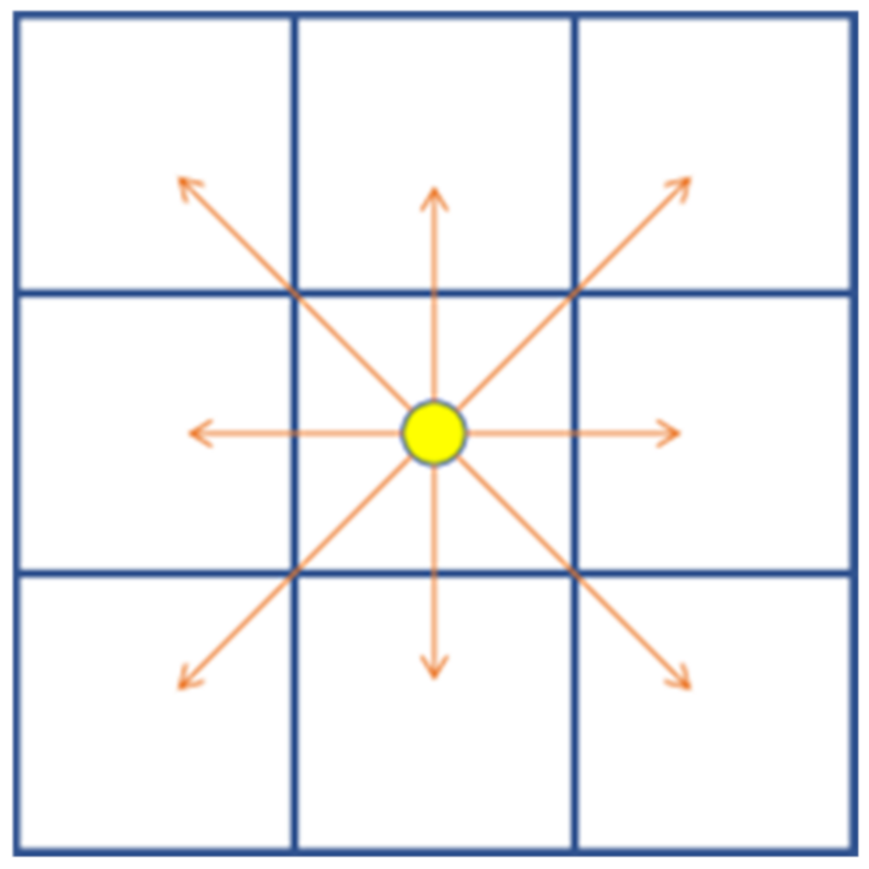
2. JPS Algorithm
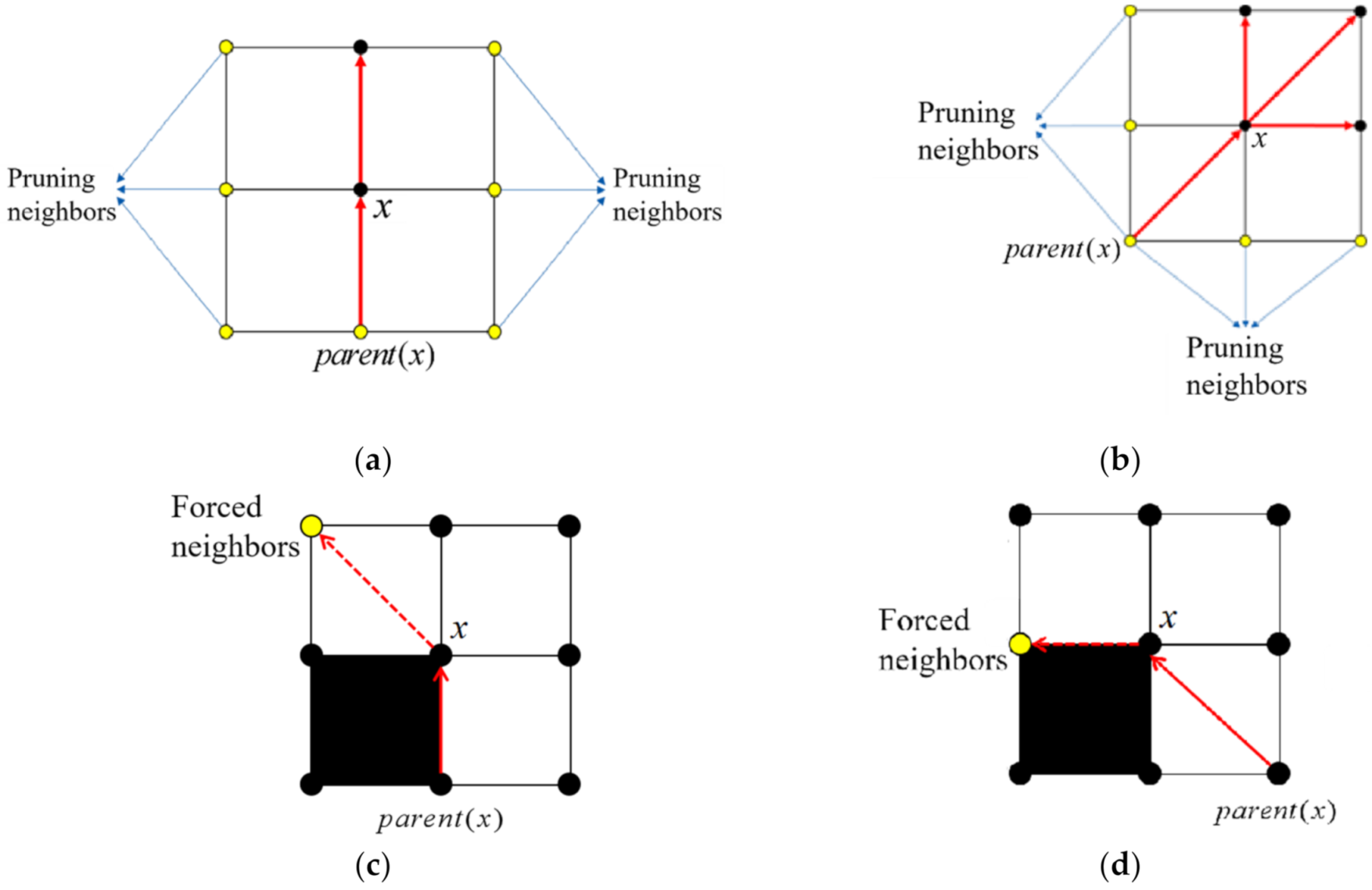
- If node is a start point or a target point, then node is a jump point.
- If node has at least one forced neighbor, then node is a jump point.
- If the search direction from the parent node of node to is diagonal and there is a point in the horizontal or vertical direction of that satisfies condition 1 and 2, then is a jump point.
JPS Algorithm for Pruned Neighbor Rule and Forced Neighbors
3. JPS Path Optimization Based on Angle-Propagation Theta* Algorithm
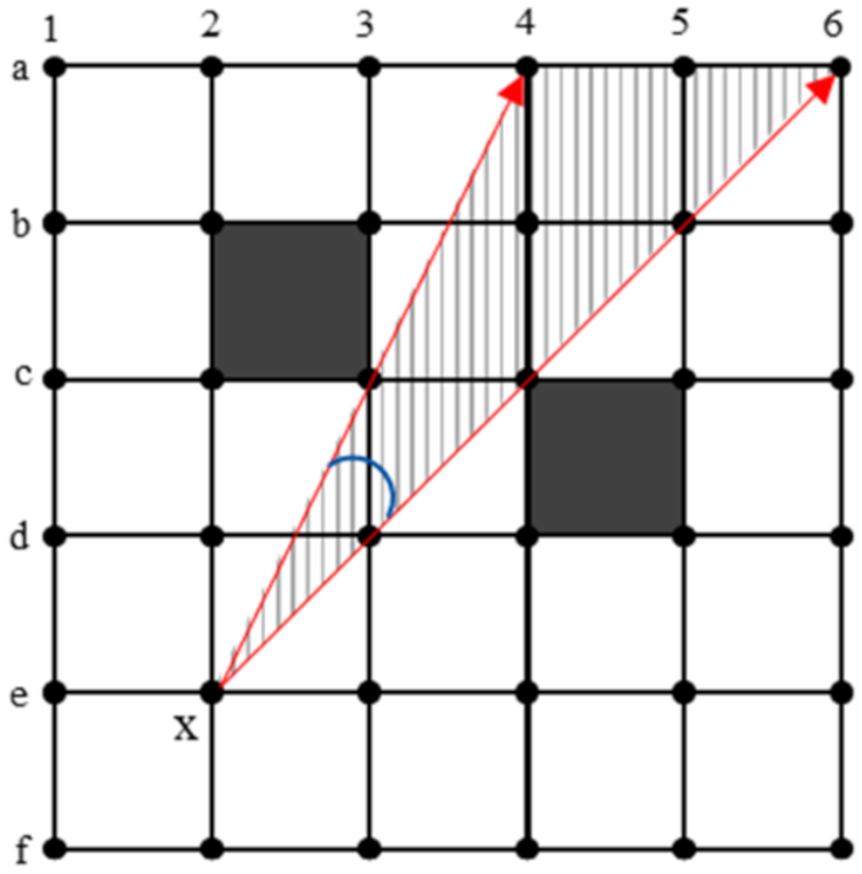
3.1. The Method of Judging the Field of Vision Triangle
3.2. Angle-Propagation Theta* Algorithm
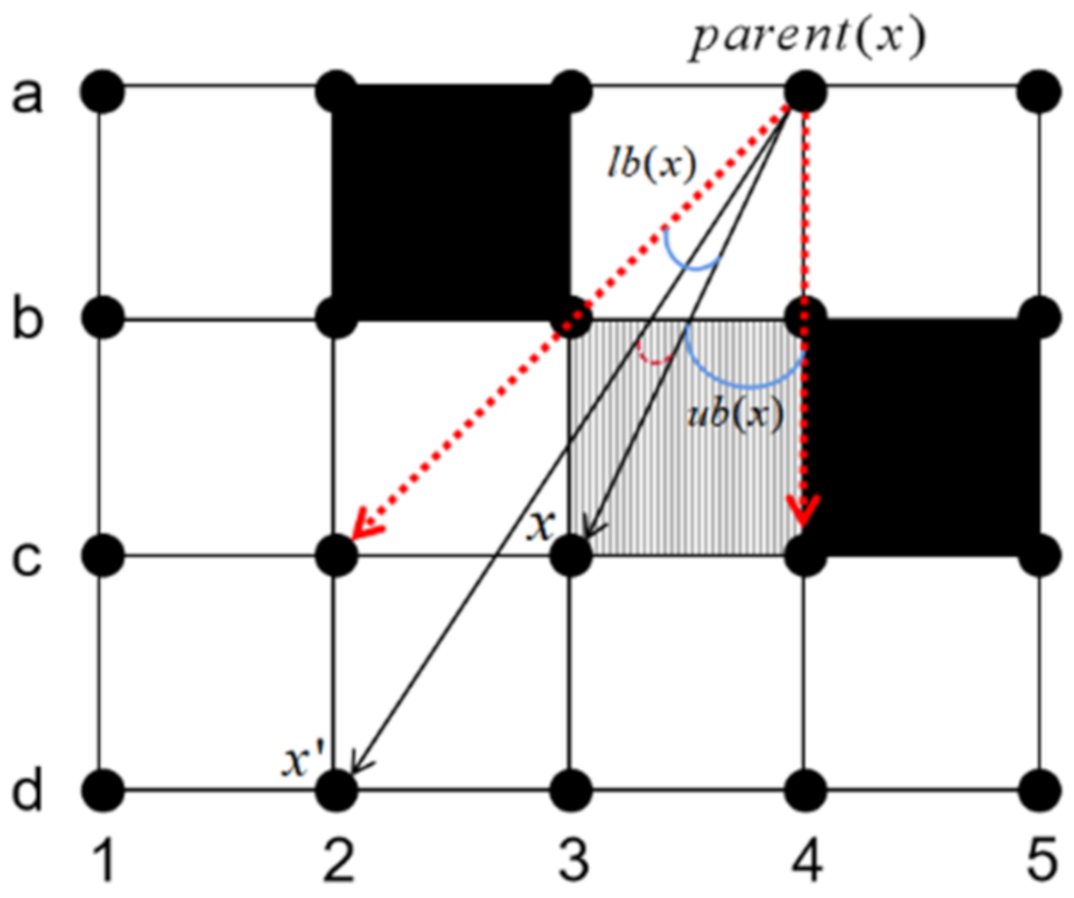
3.2.1. Definition of Angle-Propagation Theta* Algorithm Viewable Angle
3.2.2. AP-Theta* Algorithm for Visual Angle Constraint
- If the current node is a vertex of the obstacle grid and all other vertices of the current obstacle grid satisfy one of the following conditions, the lower angle region of the current node’s viewable angle area is equal to 0.If the current node is a vertex of the obstacle grid and all other vertices of the current obstacle grid satisfy one of the following conditions, the upper angle region of the current node’s viewable angle area is equal to 0.
- For a neighbor node ′ of the current node , if satisfies all of the following conditions.
- 3.
- For a neighbor node of the current node , if satisfies all of the following conditions.
| Algorithm 1: Visual Angle Constraint. |
 |
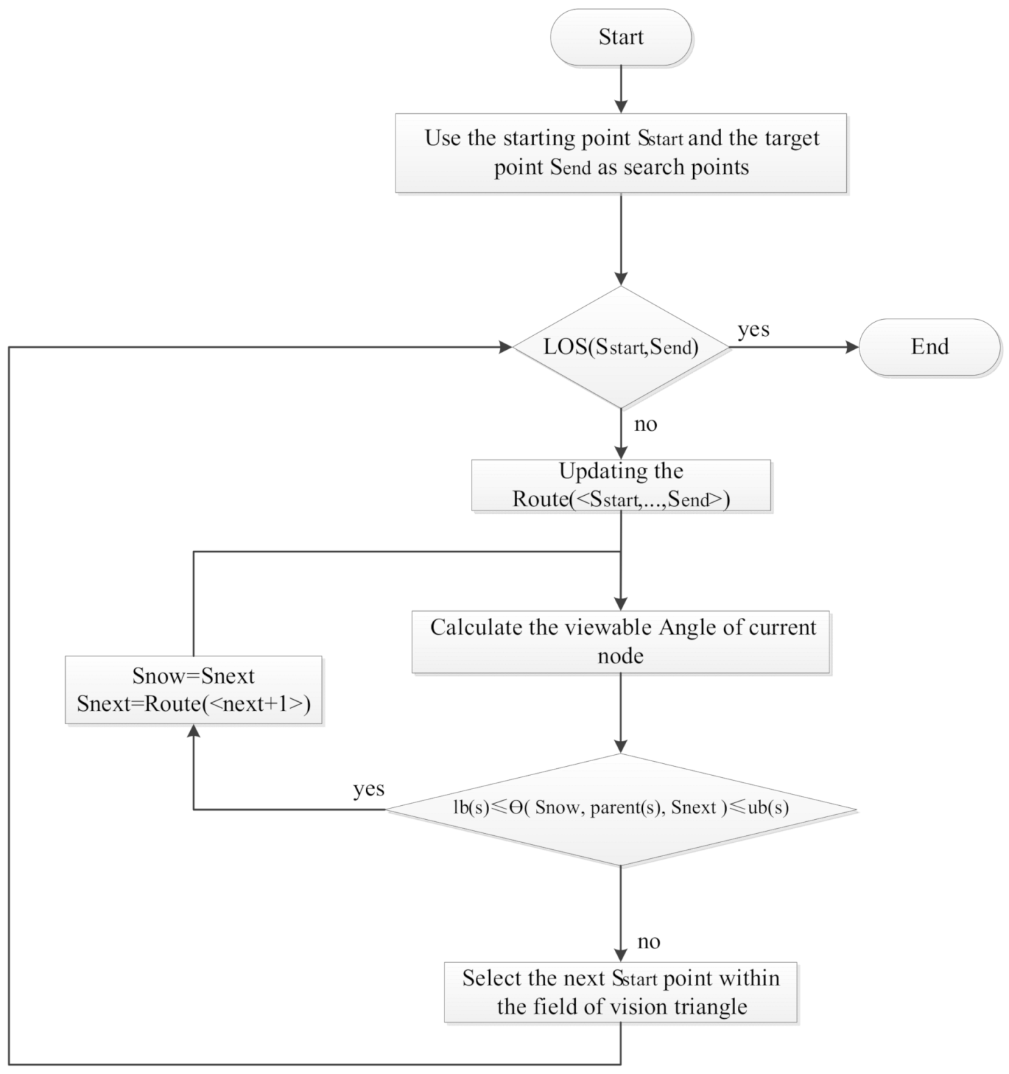
3.3. JPS Path Optimization Process with Viewable Angle Based on AP Theta *
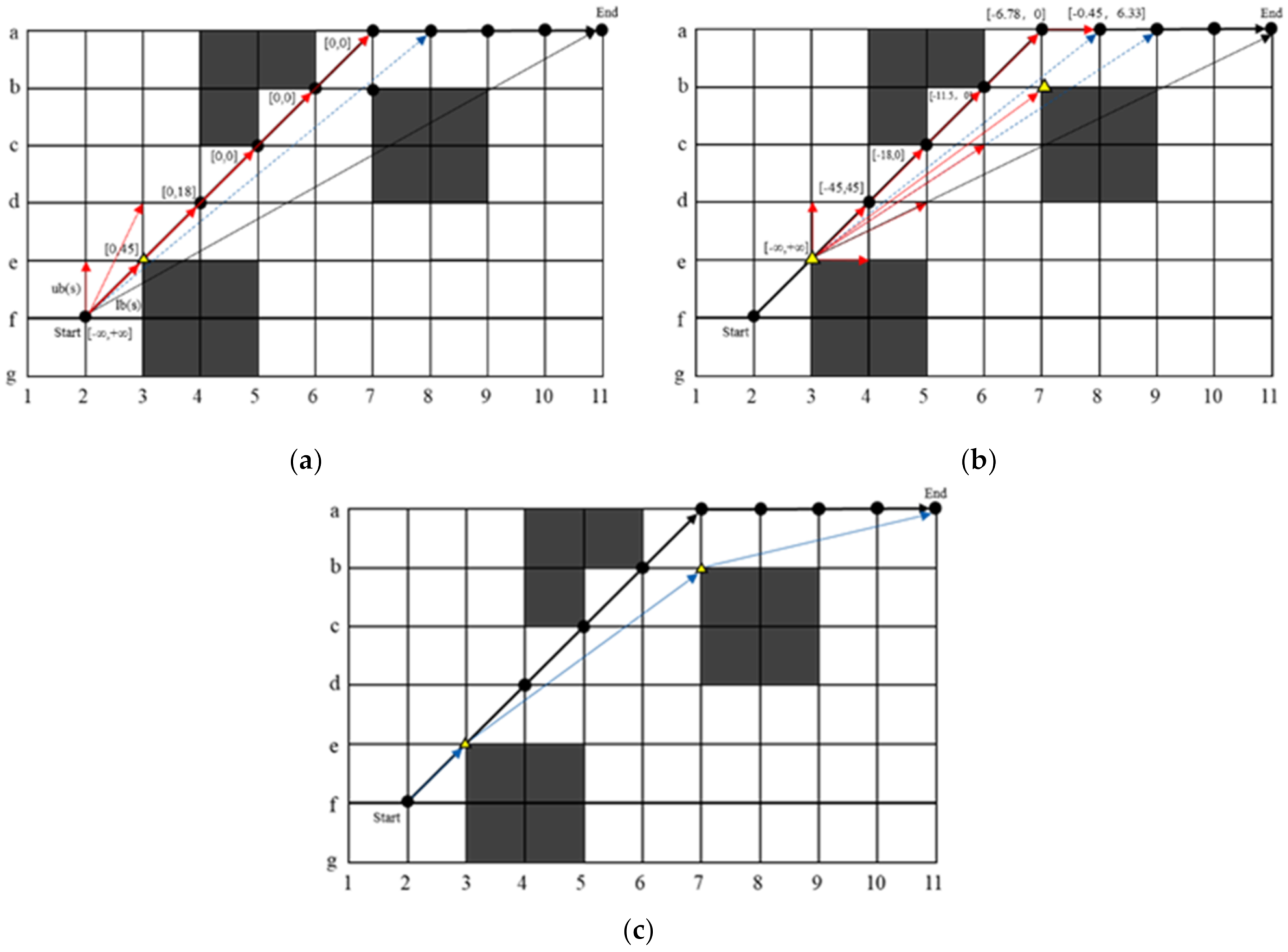
- First, the starting point (f,2) is taken as the first search point, and we judge whether there is an LOS reachable between the search point and the end point. If the LOS is reachable, the algorithm ends; if the LOS is not reachable, the path is discretized and loaded into the list. Set the child node (e,3) of the start point to the current node . Then, set the viewable range of to . Next, the constraint calculation of the viewable angle of is needed to obtain its viewable angle as [0,45]. Set the (d,4) node to in the order of the nodes in the list. The LOS reachability between all discrete points and the search point is checked in turn until the first node (a,8) is found that does not have LOS reachability, as shown in Figure 8 (1).
- Set (a,8) to flag and (a,7) to flag . The obstacle vertices within the triangular region of the field of view consisting of , and the search points are searched. The optimal turning angle (e,3) is found by calculating and comparing the cost of each vertex to the search point, as identified by the triangle in Figure 8 (1).
- Set the node (e,3) as the next search point and its path sub-node (d,4) as the current node . Continue the search by the method provided in step 1 until the next search point is found, as shown in Figure 8 (2).
- If the current search point is found to have LOS reachable with the end of the path by detection, the search is ended, as shown in Figure 8 (3). The final generated path is (f,2), (e,3), (b,7), and (a,11).
4. Trajectory Optimization
4.1. Seventh-Order Polynomial Optimization Based on Minimum Snap
4.2. Time Allocation
5. Simulation
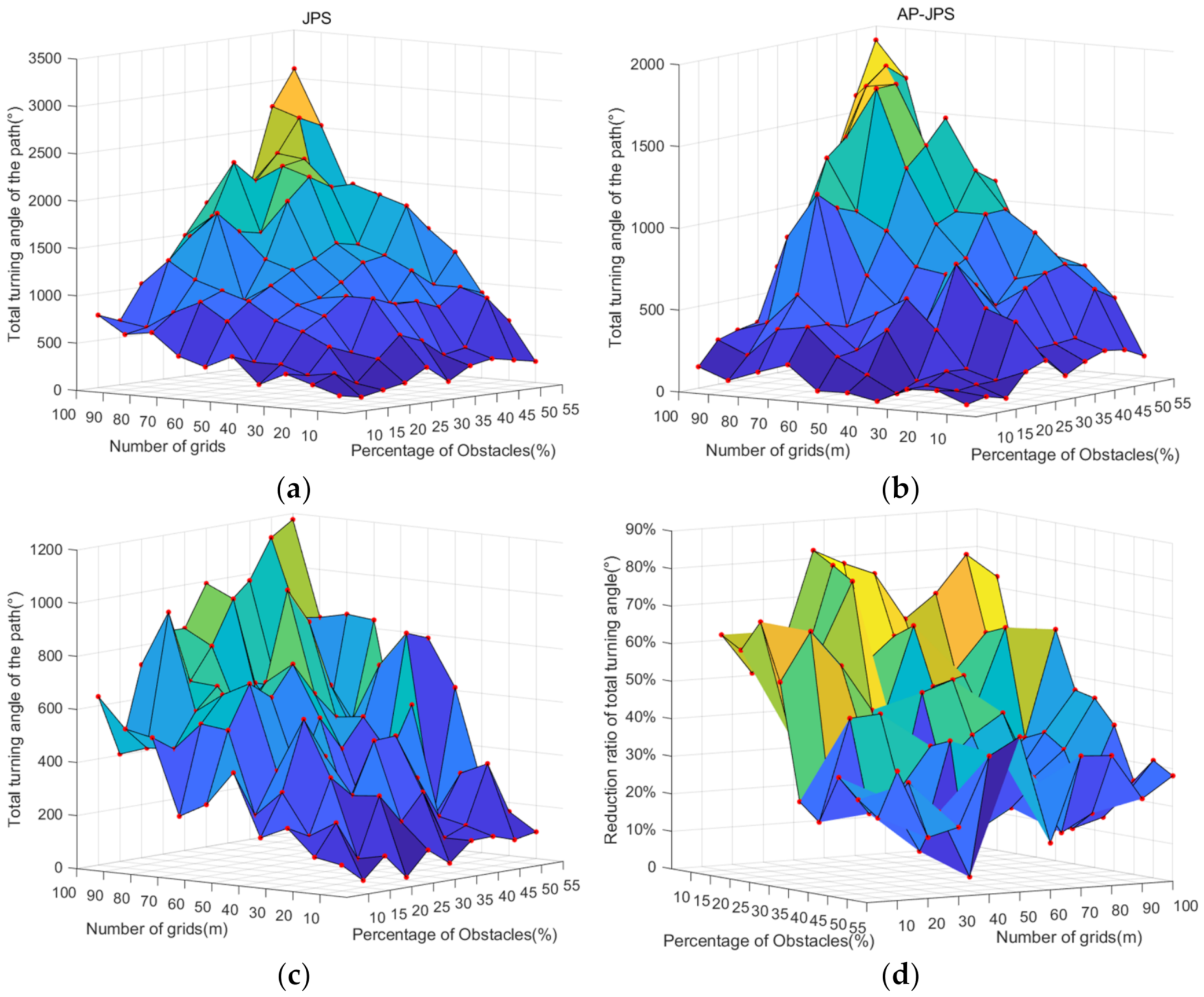
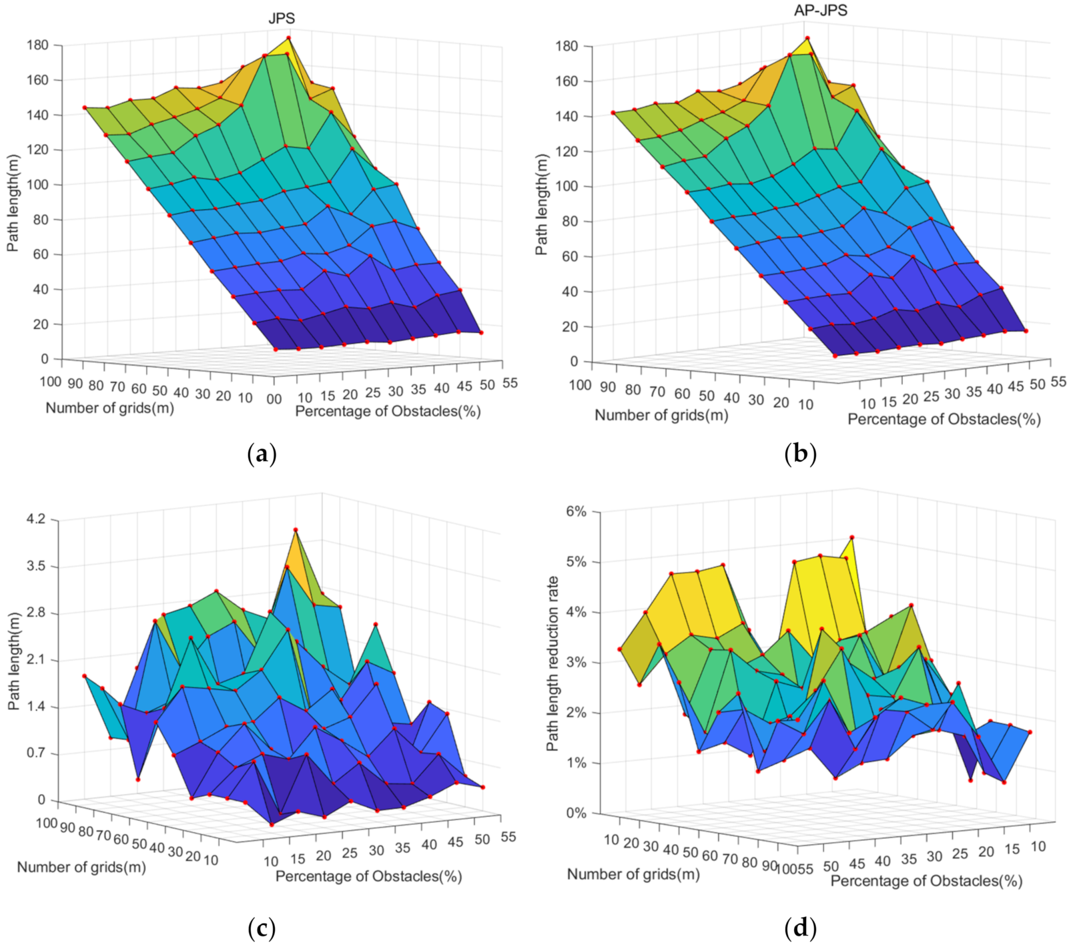
5.1. Randomness Map Test
5.2. Algorithm Comparison Experiment
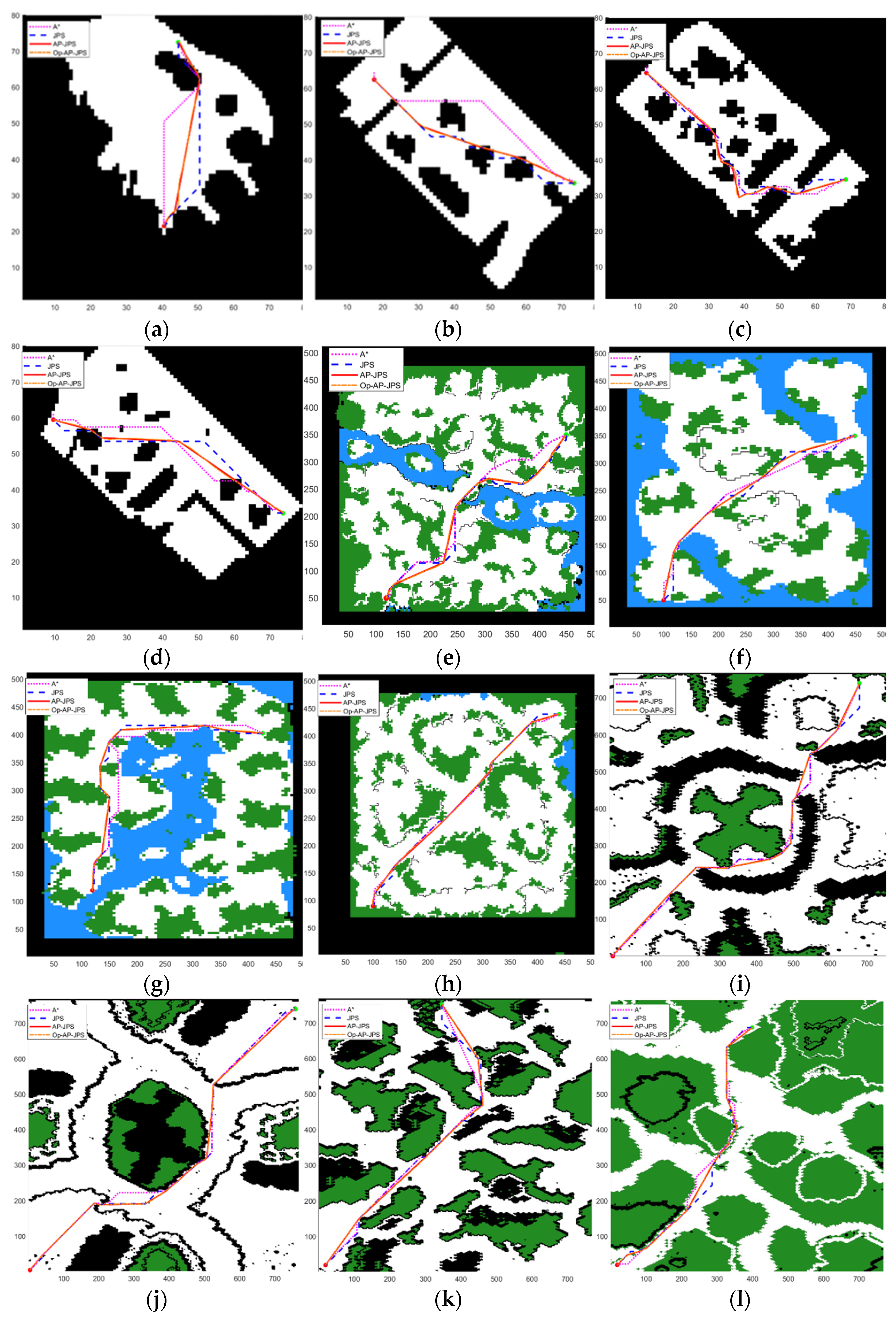
5.3. Data Set Map Experiment
6. Conclusions
- This paper proposes a smoothed JPS path planning method, combining the improved JPS algorithm with the smoothing method in this paper, adding angle indicators to the paths to exchange a smaller time sacrifice for a smoother path.
- This paper combines the AP-JPS algorithm with the seventh-order polynomial optimization based on minimum snap while introducing a safety corridor to solve the safety problem of AP-JPS optimized paths by inequality constraints.
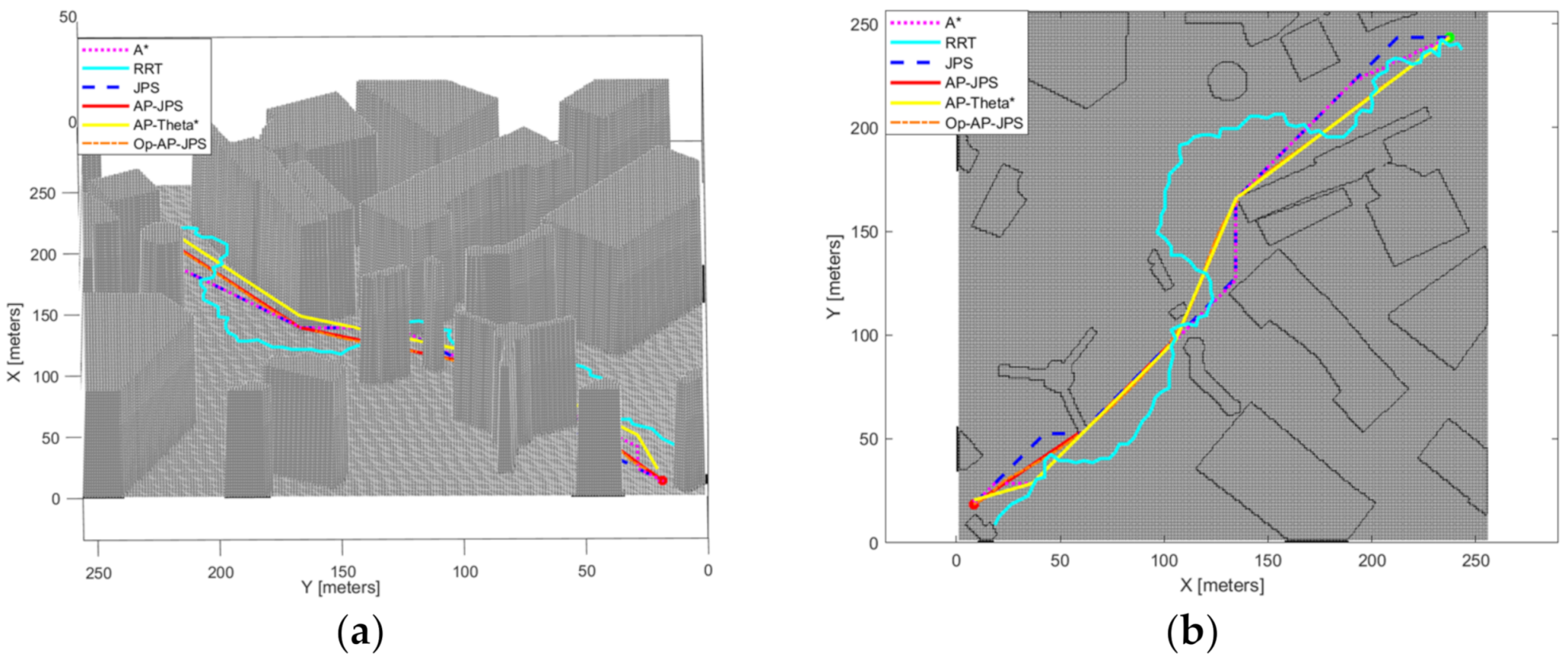
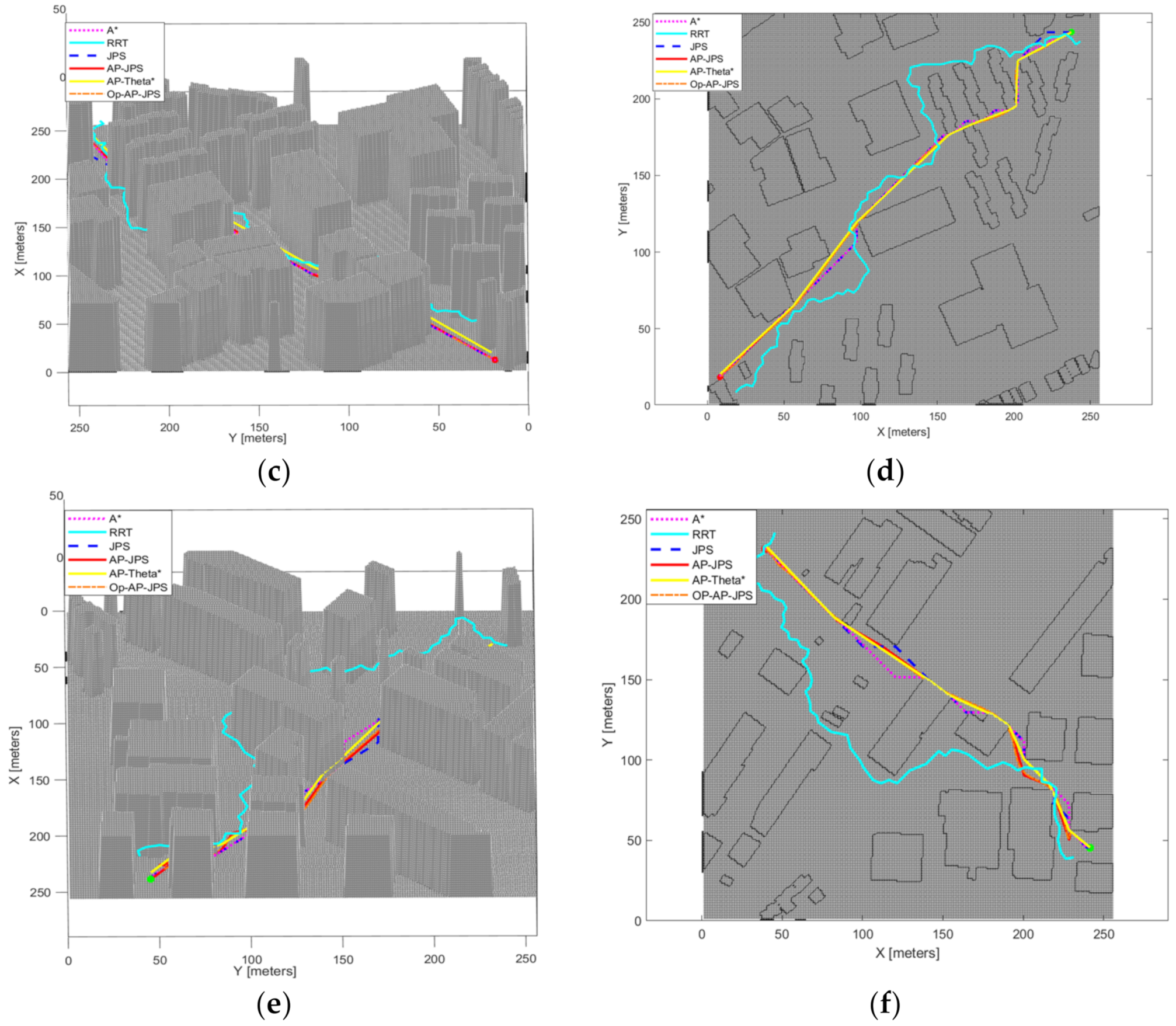
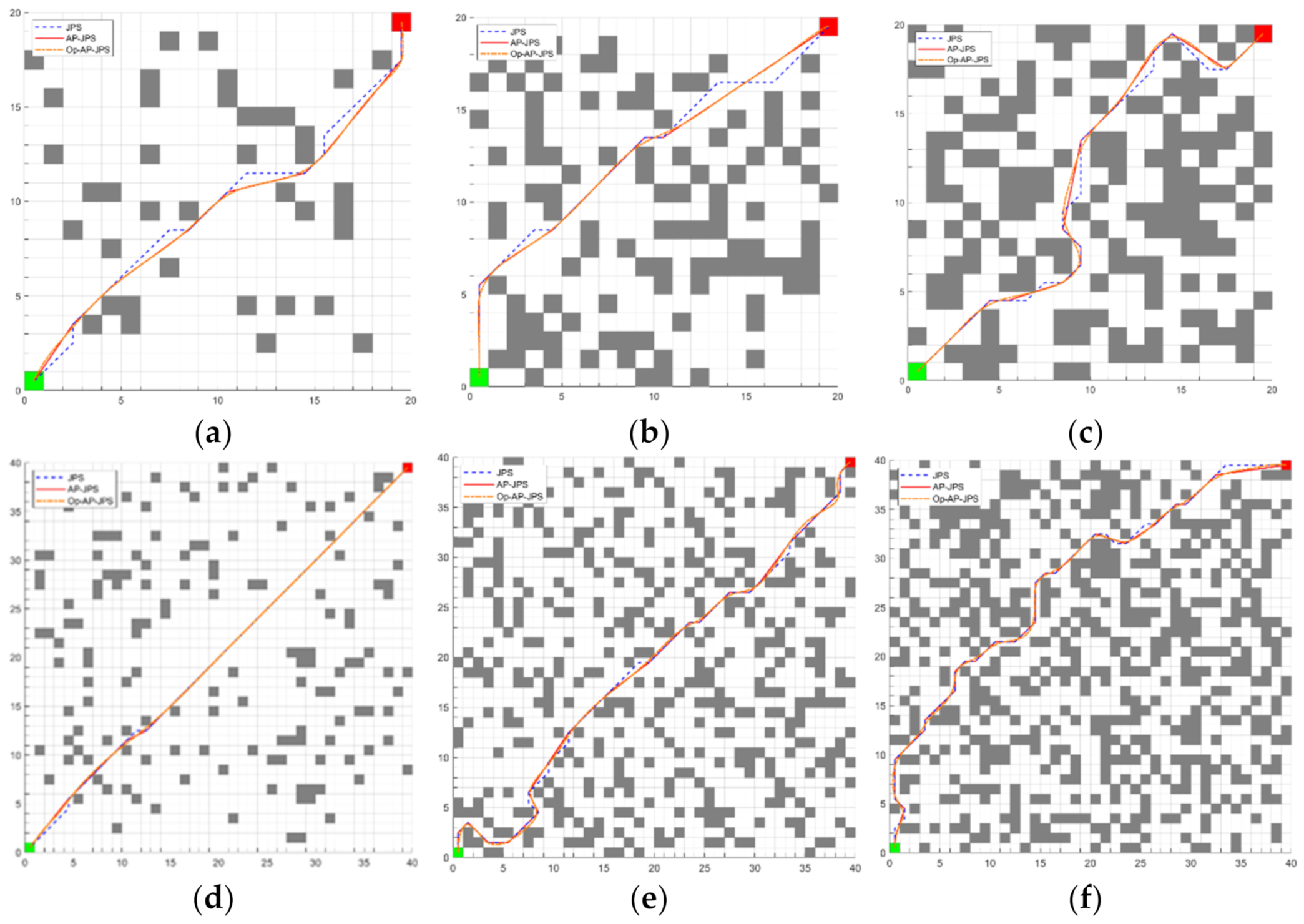
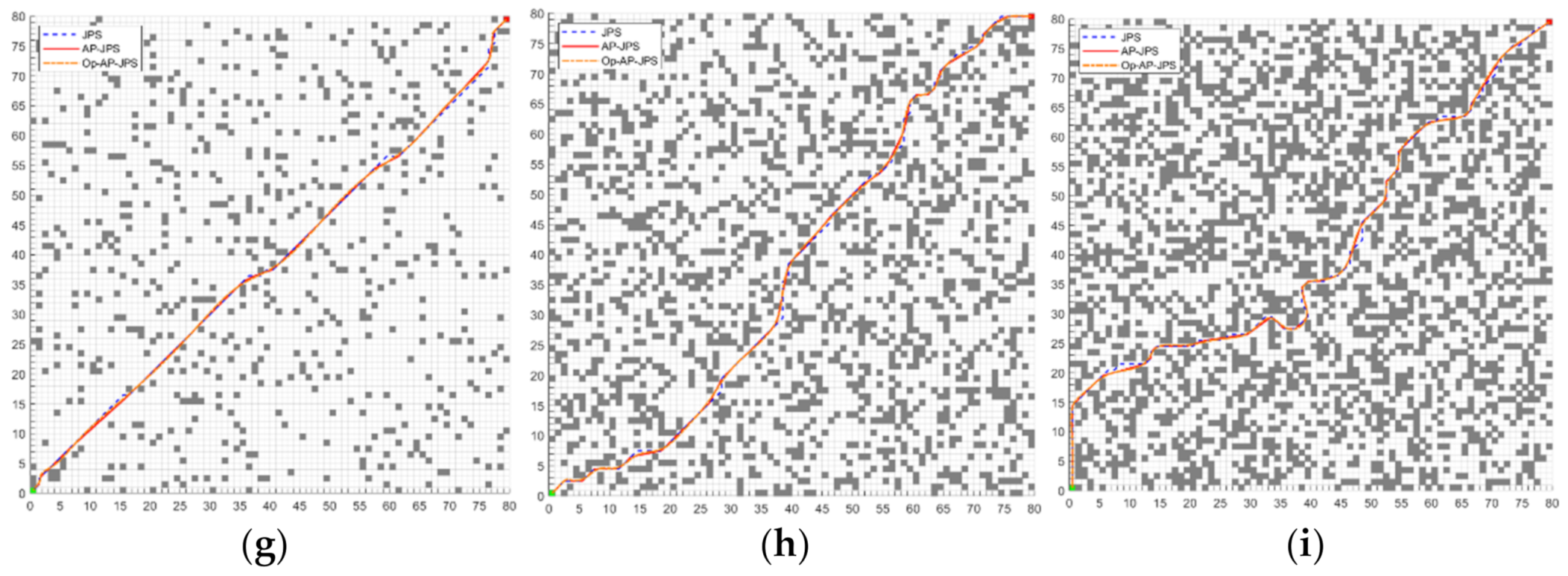
- In this paper, we verify the path optimization effect of the AP-JPS algorithm in different complex map situations by three sets of experiments. First, the AP-JPS algorithm is tested by performing the AP-JPS algorithm under different sizes of random obstacle maps. From the test results, the AP-JPS algorithm shortens the total turn angle of the path by 13.7% to 88.4% and the path length by 1.1% to 5.2% compared with the JPS algorithm. Secondly, this paper uses some map data of three cities for algorithm comparison experiments. From the experimental results, the AP-JPS algorithm has shorter and smoother paths compared to the JPS algorithm. At the same time, the time complexity and space complexity of the AP-JPS algorithm are much smaller than that of the AP-Theta* algorithm. Finally, this paper simulates real indoor and outdoor scenes by using large maps with public datasets for path planning tests. From the experimental results, the AP-JPS algorithm can complete the task with better paths, and its generated paths are more consistent with the actual motion requirements of mobile robots than other algorithms.
- The AP-JPS algorithm still has some drawbacks, as it sacrifices more computing time compared to the JPS algorithm, and the complexity of the algorithm is still high. As the size and complexity of the grid map increase, the efficiency of the algorithm decreases. In future work, we need to further optimize the computational efficiency and memory usage of AP-JPS algorithm, and we hope to apply AP-JPS 3D to UAV path planning [7].
Author Contributions
Funding
Institutional Review Board Statement
Informed Consent Statement
Data Availability Statement
Conflicts of Interest
References
- Liu, G.; Liu, Y.; Zhao, J.; Zhu, L. Path planning for a new mine rescue robot base on visual tangent graphs. Jilin Daxue Xuebao 2011, 41, 1107–1112. [Google Scholar]
- Yang, C.; Liu, Y.; Wang, Y.; Xiong, L.; Xu, H.; Zhao, W. Research and Experiment on Recognition and Location System for Citrus Picking Robot in Natural Environment. Nongye Jixie Xuebao 2019, 50, 14–22+72. [Google Scholar]
- Oh, J.S.; Choi, Y.H.; Park, J.B.; Zheng, Y.F. Complete coverage navigation of cleaning robots using triangular-cell-based map. IEEE Trans. Ind. Electron. 2004, 51, 718–726. [Google Scholar] [CrossRef]
- Atiyah, A.N.; Adzhar, N.; Jaini, N.I. An overview: On path planning optimization criteria and mobile robot navigation. J. Phys. Conf. Ser. 2021, 1988, 012036. [Google Scholar] [CrossRef]
- Babunski, D.; Berisha, J.; Zaev, E.; Bajrami, X. Application of Fuzzy Logic and PID Controller for Mobile Robot Navigation. In Proceedings of the 9th Mediterranean Conference on Embedded Computing (MECO), Budva, Montenegro, 8–11 June 2020; pp. 21–36. [Google Scholar]
- Sariff, N.; Buniyamin, N. An overview of autonomous mobile robot path planning algorithms. In Proceedings of the 4th Student Conference on Research and Development, Shah Alam, Malaysia, 27–28 June 2006; pp. 183–188. [Google Scholar]
- Zhang, N.; Zhang, M.; Low, K.H. 3D path planning and real-time collision resolution of multirotor drone operations in complex urban low-altitude airspace. Transp. Res. Part C Emerg. Technol. 2021, 129, 103123. [Google Scholar] [CrossRef]
- Ivić, S.; Crnković, B.; Grbčić, L.; Matleković, L. Multi-UAV trajectory planning for 3D visual inspection of complex structures. arXiv 2022, arXiv:math/2204.10070. [Google Scholar] [CrossRef]
- Pehlivanoglu, Y.V. A new vibrational genetic algorithm enhanced with a Voronoi diagram for path planning of autonomous UAV. Aerosp. Sci. Technol. 2012, 16, 47–55. [Google Scholar] [CrossRef]
- Ayawli, B.B.K.; Chellali, R.; Appiah, A.Y.; Kyeremeh, F. An Overview of Nature-Inspired, Conventional, and Hybrid Methods of Autonomous Vehicle Path Planning. J. Adv. Transp. 2018, 2018, 8269698. [Google Scholar]
- Zhou, K.; Yu, L.; Long, Z.; Mo, S. Local path planning of driverless car navigation based on jump point search method under urban environment. Futue Internet 2017, 9, 51. [Google Scholar] [CrossRef] [Green Version]
- Foderaro, G.; Swingler, A.; Ferrari, S. A model-based cell decomposition approach to on-line pursuit-evasion path planning and the video game Ms. Pac-Man. In Proceedings of the IEEE Conference on Computational Intelligence and Games (CIG), Granada, Spain, 11–14 September 2012; pp. 281–287. [Google Scholar]
- Hu, Q.; Wang, J.; Zhang, X. Optimized Parallel Parking Path Planning Based on Quintic Polynomial. Comput. Eng. Appl. 2022, 1–9. Available online: http://kns.cnki.net/kcms/detail/11.2127.TP.20210325.1007.008.html (accessed on 21 May 2022).
- Leiyan, Y.; Xianyu, W.; Zeyu, H.; Zaiyou, D.; Yufeng, Z.; Zhaoyang, M. Path Planning Optimization for Driverless Vehicle in Parallel Parking Integrating Radial Basis Function Neural Network. Appl. Sci. 2021, 11, 8178. [Google Scholar]
- Chen, L.; Wang, S.; Hu, H.; McDonald-Maier, K.; Fei, M. Novel path curvature optimization algorithm for intelligent wheelchair to smoothly pass a narrow space. Zidonghua Xuebao Acta Autom. Sin. 2016, 42, 1874–1885. [Google Scholar]
- Sahin, H.; Kavsaoglu, A. Indoor path finding and simulation for smart wheelchairs. In Proceedings of the 29th Signal Processing and Communications Applications Conference (SIU), Istanbul, Turkey, 9–11 June 2021; pp. 1–4. [Google Scholar]
- Hu, M.; Cao, J.; Chen, X.; Peng, F. Path planning of intelligent factory based on improved ant colony algorithm. In Proceedings of the Asia-Pacific Conference on Communications Technology and Computer Science (ACCTCS), Shenyang, China, 22–24 January 2021; pp. 1–4. [Google Scholar]
- Firmansyah, E.; Masruroh, S.; Fahrianto, F. Comparative analysis Of A and basic theta algorithm in android-based pathfmding games. In Proceedings of the 6th International Conference on Information and Communication Technology for The Muslim World (ICT4M), Jakarta, Indonesia, 22–24 November 2016; pp. 275–280. [Google Scholar]
- Geng, S.; Peng, S.; Han, Y. Research on motion planning of snake-like robot based on the interpolation function. In Proceedings of the 8th International Conference on Intelligent Human-Machine Systems and Cybernetics (IHMSC), Hangzhou, China, 27–28 August 2016; pp. 81–84. [Google Scholar]
- Huo, F.; Chi, J.; Huang, Z.; Ren, L.; Sun, Q.; Chen, J. Review of Path Planning for Mobile Robots. Jilin Daxue Xuebao 2018, 36, 639–647. [Google Scholar]
- Ravankar, A.; Ravankar, A.; Kobayashi, Y.; Hoshino, Y.; Peng, C. Path smoothing techniques in robot navigation: State-of-the-art, current and future challenges. Sensors 2018, 18, 3170. [Google Scholar] [CrossRef] [Green Version]
- Shi, J.; Su, Y.; Bu, C.; Fan, X. A mobile robot path planning algorithm based on improved A*. J. Phys. Conf. Ser. 2020, 1468, 032018. [Google Scholar] [CrossRef]
- Foo, J.L.; Knutzon, J.; Kalivarapu, V.; Oliver, J.; Winer, E. Path planning of unmanned aerial vehicles using B-splines and particle swarm optimization. J. Aerosp. Comput. Inf. Commun. 2009, 6, 271–290. [Google Scholar] [CrossRef]
- Elbanhawi, M.; Simic, M.; Jazar, R.N. Continuous Path Smoothing for Car-Like Robots Using B-Spline Curves. J. Intell. Robot. Syst. Theor. Appl. 2015, 80, 23–56. [Google Scholar] [CrossRef]
- Huh, U.-Y.; Chang, S.A. G2 continuous path-smoothing algorithm using modified quadratic polynomial interpolation. Int. J. Adv. Rob. Syst. 2014, 11, 25. [Google Scholar] [CrossRef]
- Liu, S.; Watterson, M.; Mohta, K.; Sun, K.; Bhattacharya, S.; Taylor, C.J.; Kumar, V. Planning dynamically feasible trajectories for quadrotors using safe flight corridors in 3-D complex environments. IEEE Robot. Autom. 2017, 2, 1688–1695. [Google Scholar] [CrossRef]
- Harabor, D.; Grastien, A. Online graph pruning for pathfinding on grid maps. In Proceedings of the AAAI Conference on Artificial Intelligence, San Francisco, CA, USA, 7–11 August 2011; Volume 25, pp. 1114–1119. [Google Scholar]
- Huang, J.; Wu, Y.; Lin, X. Smooth JPS Path Planning and Trajectory Optimization Method of Mobile Robot. Nongye Jixie Xuebao 2021, 52, 21–29+121. [Google Scholar]
- Dave, F.; Anthony, S. Field D*: An Interpolation-Based Path Planner and Replanner; Robotics Research; Springer: Berlin/Heidelberg, Germany, 2007; pp. 239–253. [Google Scholar]
- Daniel, K.; Nash, A.; Koenig, S.; Felner, A. Theta*: Any-Angle Path Planning on Grids. JAIR 2010, 39, 533–579. [Google Scholar] [CrossRef] [Green Version]
- Sinyukov, D.A.; Padir, T. CWave: Theory and Practice of a Fast Single-source Any-angle Path Planning Algorithm. Robotica 2020, 38, 207–234. [Google Scholar] [CrossRef]
- Jayasree, K.; Jayasree, P.; Vivek, A. Smoothed RRT techniques for trajectory planning. In Proceedings of the International Conference on Technological Advancements in Power and Energy (TAP Energy), Kollam, India, 21–23 December 2017; Volume 1, pp. 1–8. [Google Scholar]
- Chen, L.; Shan, Y.; Tian, W.; Li, B.; Cao, D. A Fast and Efficient Double-Tree RRT*-Like Sampling-Based Planner Applying on Mobile Robotic Systems. IEEE ASME Trans. Mechatron. 2018, 23, 2568–2578. [Google Scholar] [CrossRef]
- Gammel, J.; Srinivasa, S.; Barfoot, T. Informed RRT*: Optimal sampling-based path planning focused via direct sampling of an admissible ellipsoidal heuristic. In Proceedings of the IEEE/RSJ International Conference on Intelligent Robots and Systems, Chicago, IL, USA, 14–18 September 2014; pp. 2997–3004. [Google Scholar]
- Yao, Q.; Zheng, Z.; Qi, L.; Yuan, H.; Guo, X.; Zhao, M.; Liu, Z.; Yang, T. Path Planning Method with Improved Artificial Potential Field–A Reinforcement Learning Perspective. IEEE Access 2020, 8, 135513–135523. [Google Scholar] [CrossRef]
- Liu, Z.; Yu, L.; Xiang, Q.; Qian, T.; Lou, Z.; Xue, W. Research on USV trajectory tracking method based on LOS algorithm. In Proceedings of the 14th International Symposium on Computational Intelligence and Design (ISCID), Hangzhou, China, 11–12 December 2021; Volume 1, pp. 408–411. [Google Scholar]


| Classification | Algorithm | Problems |
|---|---|---|
| Path planning methods | A* Algorithm | The A* algorithm has a large number of redundant nodes in the search process leading to the inefficiency of the algorithm, especially when the map size is large. |
| RRT algorithm [32] | The RRT algorithm is particularly important for the design of the step length. A step length that is too long leads to crossing obstacles. Too short a step length leads to inefficiency of the algorithm. In addition, the path found by the RRT algorithm is suboptimal, not optimal. | |
| RRT* algorithm [33] | The RRT* algorithm is asymptotically optimized, which means that the resulting path is increasingly optimized as the number of iterations increases [34]. Therefore, the convergence time of the RRT* algorithm is a more prominent problem. | |
| Artificial potential field [35] | The combined force generated by the gravitational field and the repulsive field is zero; then, it is easy to fall into the local optimum solution. | |
| JPS algorithm | The fixed direction search results in a gap between the resulting path and the path available to the mobile robot. | |
| Path smoothing method | Bessel curve optimization | The Bessel curve is less flexible, and the generated path does not guarantee the continuity of velocity and acceleration. |
| B-sample curve optimization | The B spline curve is more flexible than the Bessel curve because of its local modifiable feature. However, the optimized path still cannot guarantee the continuity of velocity and acceleration. | |
| Polynomial interpolation method | The polynomial interpolation method is better for continuity treatment, but the possibility of reoccurrence of collisions in the fitted curves needs to be taken into account. | |
| Any-angle path planning method | Line of sight method [29] | The line-of-sight method is inefficient for optimization and requires LOS detection for a large number of nodes, leading to a decrease in the efficiency of the algorithm. |
| Field D* | The path obtained by the Field D* algorithm is not the optimal path. | |
| Basic Theta* | The time required by the Basic Theta* algorithm to expand each vertex increases linearly with the number of rasters. When the map size is too large, the algorithm becomes less efficient. | |
| AP-Theta* | Although the consumption of AP Theta* in expanding vertices is no longer linearly related to the number of lattices, but becomes constant in magnitude. However, the search process of a large number of useless nodes still exists in the Theta* family of algorithms, resulting in inefficiency |
| Name | Running Time (s) | Memory Usage (kb) | Path Length (m) | Total Turning Angle of the Path (°) | |
|---|---|---|---|---|---|
| Shanghai | A* | 28.3386 | 2488.4063 | 345.0437 | 2160 |
| RRT | 99.5774 | 536.7510 | 472.1204 | 4205.3070 | |
| JPS | 0.1217 | 1067.0938 | 345.0437 | 405 | |
| AP-Theta* | 29.0491 | 2740.0223 | 349.2478 | 154.3191 | |
| AP-JPS | 0.2265 | 1224.1230 | 328.8865 | 94.3191 | |
| New York | A* | 19.4580 | 2410.4219 | 346.2153 | 2430 |
| RRT | 104.9274 | 547.0947 | 464.1386 | 4004.6040 | |
| JPS | 0.1659 | 1111.2578 | 346.2153 | 1125 | |
| AP-Theta* | 21.4166 | 2715.2300 | 334.7146 | 172.4967 | |
| AP-JPS | 0.2889 | 1363.1390 | 334.7146 | 172.4967 | |
| Boston | A* | 11.7563 | 1990.7422 | 294.8600 | 1305 |
| RRT | 61.5348 | 533.3369 | 415.6851 | 2904.0880 | |
| JPS | 0.1074 | 1065.6250 | 294.8600 | 1125 | |
| AP-Theta* | 13.2568 | 2275.0470 | 290.1114 | 464.5372 | |
| AP-JPS | 0.1864 | 1280.2889 | 290.1114 | 464.5372 | |
| Number | Map Name | Map Size (m) | Number of Obstacles | Max Length Problem in Scenario | |
|---|---|---|---|---|---|
| 1 | Baldurs Gate II | AR0513SR | 80 × 80 | 4328 | 87.1543 |
| 2 | AR0709SR | 80 × 80 | 4353 | 75.0121 | |
| 3 | AR0310SR | 80 × 80 | 4517 | 62.6274 | |
| 4 | AR0704SR | 80 × 80 | 4752 | 95.2548 | |
| 5 | Warcraft III | divideandconquer | 512 × 512 | 146,545 | 651.3280 |
| 6 | plunderisle | 512 × 512 | 147,100 | 654.7077 | |
| 7 | harvestmoon | 512 × 512 | 147,551 | 567.9331 | |
| 8 | moonglade | 512 × 512 | 159,833 | 682.7544 | |
| 9 | Starcraft | Crossroads | 768 × 768 | 200,600 | 1183.8053 |
| 10 | BlastFurnace | 768 × 768 | 205,689 | 1355.3890 | |
| 11 | Hellfire | 768 × 768 | 273,180 | 1211.3006 | |
| 12 | SapphireIsles | 768 × 768 | 380,719 | 1443.8986 | |
| Number | Map Name | Algorithm Type | Path Length (m) | Total Turning Angle of the Path (°) | Operation Time (s) |
|---|---|---|---|---|---|
| 1 | AR0513SR | A* | 68.0122 | 315 | 0.1654 |
| 2 | JPS | 68.0122 | 315 | 0.0397 | |
| 3 | AP-JPS | 64.3672 | 39.5076 | 0.0751 | |
| 4 | AR0709SR | A* | 74.7696 | 495 | 0.2241 |
| 5 | JPS | 74.7696 | 225 | 0.0248 | |
| 6 | AP-JPS | 71.4807 | 104.1320 | 0.0643 | |
| 7 | AR0310SR | A* | 57.6233 | 585 | 0.1523 |
| 8 | JPS | 57.6233 | 225 | 0.0137 | |
| 9 | AP-JPS | 54.3827 | 94.3987 | 0.0674 | |
| 10 | AR0704SR | A* | 78.0833 | 990 | 0.2057 |
| 11 | JPS | 78.0833 | 675 | 0.0303 | |
| 12 | AP-JPS | 77.6401 | 378.6445 | 0.0988 |
| Number | Map Name | Algorithm Type | Path Length (m) | Total Turning Angle of the Path (°) | Operation Time (s) |
|---|---|---|---|---|---|
| 1 | divideandconquer | A* | 502.7838 | 2690 | 93.6902 |
| 2 | JPS | 527.5706 | 1035 | 3.9906 | |
| 3 | AP-JPS | 500.2249 | 291.3104 | 7.9424 | |
| 4 | plunderisle | A* | 519.9554 | 891 | 100.7357 |
| 5 | JPS | 519.9554 | 765 | 3.8260 | |
| 6 | AP-JPS | 492.9167 | 80.2559 | 5.9129 | |
| 7 | harvestmoon | A* | 516.2641 | 2430 | 90.5687 |
| 8 | JPS | 516.2641 | 855 | 4.0340 | |
| 9 | AP-JPS | 503.5609 | 182.1982 | 5.9667 | |
| 10 | moonglade | A* | 589.3209 | 2745 | 90.1968 |
| 11 | JPS | 589.3209 | 1035 | 4.6622 | |
| 12 | AP-JPS | 570.7837 | 288.7079 | 7.1101 |
| Number | Map Name | Algorithm Type | Path Length (m) | Total Turning angle of the Path (°) | Operation Time (s) |
|---|---|---|---|---|---|
| 1 | Crossroads | A* | 1175.8 | 4140 | 793.3247 |
| 2 | JPS | 1175.8 | 2385 | 8.4912 | |
| 3 | AP-JPS | 1151.4 | 412.6626 | 15.9326 | |
| 4 | BlastFurnace | A* | 1136.5 | 4200 | 781.1085 |
| 5 | JPS | 1136.5 | 1665 | 9.5450 | |
| 6 | AP-JPS | 1097.0 | 359.3899 | 16.5546 | |
| 7 | Hellfire | A* | 980.7048 | 1039 | 717.4127 |
| 8 | JPS | 980.7048 | 675 | 15.4673 | |
| 9 | AP-JPS | 948.6092 | 144.3275 | 24.5147 | |
| 10 | SapphireIsles | A* | 884.8154 | 3690 | 561.7834 |
| 11 | JPS | 884.8154 | 1165 | 12.2100 | |
| 12 | AP-JPS | 851.2148 | 419.2467 | 21.2617 |
Publisher’s Note: MDPI stays neutral with regard to jurisdictional claims in published maps and institutional affiliations. |
© 2022 by the authors. Licensee MDPI, Basel, Switzerland. This article is an open access article distributed under the terms and conditions of the Creative Commons Attribution (CC BY) license (https://creativecommons.org/licenses/by/4.0/).
Share and Cite
Luo, Y.; Lu, J.; Qin, Q.; Liu, Y. Improved JPS Path Optimization for Mobile Robots Based on Angle-Propagation Theta* Algorithm. Algorithms 2022, 15, 198. https://doi.org/10.3390/a15060198
Luo Y, Lu J, Qin Q, Liu Y. Improved JPS Path Optimization for Mobile Robots Based on Angle-Propagation Theta* Algorithm. Algorithms. 2022; 15(6):198. https://doi.org/10.3390/a15060198
Chicago/Turabian StyleLuo, Yuan, Jiakai Lu, Qiong Qin, and Yanyu Liu. 2022. "Improved JPS Path Optimization for Mobile Robots Based on Angle-Propagation Theta* Algorithm" Algorithms 15, no. 6: 198. https://doi.org/10.3390/a15060198
APA StyleLuo, Y., Lu, J., Qin, Q., & Liu, Y. (2022). Improved JPS Path Optimization for Mobile Robots Based on Angle-Propagation Theta* Algorithm. Algorithms, 15(6), 198. https://doi.org/10.3390/a15060198