Article

Process Mining the Performance of a Real-Time Healthcare 4.0 Systems Using Conditional Survival Models

by
Adele H. Marshall
1,2,*,† and
Aleksandar Novakovic
1,2,*,†
1
School of Mathematics and Physics, Queen’s University Belfast, University Road, Belfast BT7 1NN, Northern Ireland, UK
2
Joint Research Centre in AI for Health and Wellness, Faculty of Business and IT, Ontario Tech University, 2000 Simcoe Street North, Oshawa, ON L1G 0C5, Canada
*
Authors to whom correspondence should be addressed.
These authors contributed equally to this work.
Algorithms 2022, 15(6), 196; https://doi.org/10.3390/a15060196
Submission received: 14 May 2022 / Revised: 1 June 2022 / Accepted: 5 June 2022 / Published: 7 June 2022
(This article belongs to the Special Issue Process Mining and Its Applications)

Abstract

:
As the world moves into the exciting age of Healthcare 4.0, it is essential that patients and clinicians have confidence and reassurance that the real-time clinical decision support systems being used throughout their care guarantee robustness and optimal quality of care. However, current systems involving autonomic behaviour and those with no prior clinical feedback, have generally to date had little focus on demonstrating robustness in the use of data and final output, thus generating a lack of confidence. This paper wishes to address this challenge by introducing a new process mining approach based on a statistically robust methodology that relies on the utilisation of conditional survival models for the purpose of evaluating the performance of Healthcare 4.0 systems and the quality of the care provided. Its effectiveness is demonstrated by analysing the performance of a clinical decision support system operating in an intensive care setting with the goal to monitor ventilated patients in real-time and to notify clinicians if the patient is predicted at risk of receiving injurious mechanical ventilation. Additionally, we will also demonstrate how the same metrics can be used for evaluating the patient quality of care. The proposed methodology can be used to analyse the performance of any Healthcare 4.0 system and the quality of care provided to the patient.

1. Introduction

Process Mining is described as the body of work that focuses on the extraction of knowledge and the analysis of processes from routinely collected data or that generated and stored in corporate information systems [1]. Most broadly the attention of process mining has been within business processes but more recently, in the past 10 years, this application has been extended to healthcare. Rojas et al. [1] conducted a comprehensive literature review of case studies and the main approaches used in the application of process mining in the healthcare domain. In particular they highlight the benefits of process mining in allowing healthcare providers the ability to better understand their systems, the execution of their processes, their conformance checking of medical guidelines, and with this identify opportunities for improvement. Out of the approaches listed in the literature, to date, none have considered the use of conditional survival analysis approaches and it is with this in mind that we propose the methodology in this paper.
When patients are in a critical state, they are admitted to the intensive care unit (ICU) so that their vital signs can be carefully monitored and the most suitable treatment provided to the patient in a timely manner. The patient vital signs are measurements used to reflect the state of the patient’s essential body functions. The most commonly recorded are patient body temperature, blood pressure, pulse, and respiration rate. Any change in these measurements suggests a change in the patient condition, or could indicate the severity of patient illness and level of urgency for treatment [2].
The vast majority of instruments used for monitoring vital signs and providing organ support in ICU settings, usually have the capability of emitting patients’ physiological readings in the format that is compatible with the Health Level 7 (HL7) standards, which define the guidelines for data exchange, the retrieval and the sharing of patient electronic health information, all of which are important to ensure that the various systems integrate seamlessly [2,3]. The data outputs from these devices are usually stored inside the Electronic Medical Records (EMRs) for the purpose of monitoring and analysing the patients’ changing conditions over time [4,5,6]. The complexity of having data flowing continuously from a number of data sources in a dynamically changing environment drives the need to have appropriate clinical responses in real-time. However, clinicians in ICUs normally have to make thousands of decisions per day, resulting in between 80 to 200 interventions daily per patient, only one of which is caring about providing adequate quality of mechanical ventilation. Hence, too many data points and types can lead to information overload where healthcare providers are faced with challenges in trying to make sense of the data in high volumes, leading to clinicians’ cognitive overload. As a result, clinicians and healthcare providers can have a slow and possibly inconsistent response [7], which in turn can impact negatively on patient outcomes by for example reducing patient survival rates, or extending the period of organ support for the patients.
One of the most often used devices for providing organ support are mechanical ventilators, which provide breathing assistance to patients who develop respiratory failures. Preclinical and clinical trials concerning ventilated animal and human subjects respectively provide evidence that if ventilation is not correctly performed it may become a harmful intervention, which can permanently damage a patient’s lungs [8]. This injurious ventilation to the lungs is known as ventilator induced lung injury (VILI) and can be experienced not just by patients with respiratory failures, but also by patients with healthy lungs [9]. Lung protective ventilation (LPV) strategies have been introduced to prevent such harmful effects of ventilation, whereby it is recommended that patients should be ventilated with low tidal volumes typically less than 8 mL/kg of ideal body weight (IBW) [10,11,12].
Although there has been a significant volume of work in illustrating the positive aspects of LPV, evidence suggests that at most only half of such ventilated patients undergo LPV in a clinical environment [13,14,15]. The need for appropriate use of LPV, inspired our earlier work on VILIAlert when we created a clinical decision support system (CDS) with real-time smart alerting capabilities, and Healthcare 4.0 compliance. Its first deployment has been in Belfast’s Royal Victoria Hospital, where the vision is to have a continuous monitoring system of a patient’s tidal volume (TV), which is evaluated using a set of thresholds from which appropriate real time alerts are triggered if there is a predicted risk of VILI occurring. The ICU in which it was implemented has a maximum capacity for 20 patients and an aspect of earlier research has demonstrated the feasibility of adopting VILIAlert to scale up to a hospital wide scenario [16].
When an alert is raised, it is a major challenge of such smart-alerting CDSs to be able to determine whether the alert is considered to be genuine or not without expert opinion. However, referring every case to the expert, has the potential of causing expert alert fatigue or complacency for the alerts, undermining the whole purpose of the alerts and value [17]. Because of this issue, and due to clinicians’ competing work demands, the accuracy assessment is often performed at the end of the study, by manually inspecting each generated alert so a decision can be made on whether they are genuine or not. The main issue with this retrospective performance assessment approach is that it is a very difficult and time consuming process, particularly if we take into account that over time, this can lead to a huge number of generated alerts being accumulated, which highly depends on the quality of alerting algorithm, the number of patients that are involved in the study, and other CDS settings. Therefore, this raises a need for new accuracy assessment techniques, which should accelerate development of novel smart alerting algorithms and lead towards minimising reliance on clinical assistance [6]. In our earlier work, we created the DM-P approach to address this somewhat unsupervised learning challenge where the data generated from the alerts is unlabelled and there is no further information as to whether the alert is genuine or not. The DM in the approach refers to the new defects map method of visualising the alerts, which is combined with p-charts, a type of statistical process control (SPC) charts used in quality control of dichotomous processes, similar in nature to the dichotomous variable of an alert being raised or not. This work had been inspired by Bourdeaux et al. [18] who previously illustrated that if the alert was triggered for the TV values greater than 8 mL/kg, these values continue to remain above this threshold until there is clinical intervention. The DM-P approach can be used as a standalone independent module or can be used in conjunction with other healthcare systems.
In this current paper, we use the same hypothesis as in our earlier work, that is, the assumption that if the alert was triggered because the TV readings violated the 8 mL/kg threshold, then it is expected that this threshold is going to be continuously violated for some considerable time in the future until there is clinical intervention. We propose an approach based on conditional survival analysis techniques that enables researchers to dynamically estimate the probabilities that will describe for how long this hypothesis will hold the ground truth, suggesting that the longer survival times indicates a better algorithm performance and poorer quality of care. To the best of our knowledge, conditional survival analysis techniques have never before been utilised in this context nor was it possible to achieve this using the DM-P approach.
The paper is structured using the following sections. Section 2 describes the VILIAlert system architecture, and establishes the theoretical fundamentals that are required when using survival analytics to evaluate the performance of unlabelled datasets in real-time. Section 3 provides the results of applying the techniques established in Section 2 to the VILIAlert data set and Section 4 discusses the research outcomes illustrating the advantages and disadvantages of the proposed survival analytics based evaluation techniques, and the potential further research to follow. To conclude, Section 5 provides our final closing statements on the research in this paper.

2. Methods

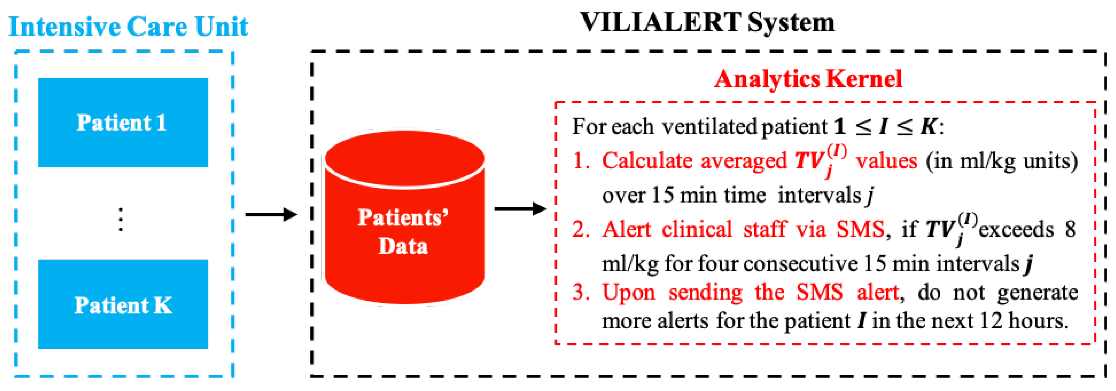
2.1. The VILIAlert System Architecture

The VILIAlert system was deployed to operate in parallel with the EMR to monitor the ventilation process in continuous time and is therefore relevant for process mining. Its purpose is to notify clinicians when there is a high risk of VILI in ventilated patients. Such risk is according to the configured settings of the system. Its design consists of two components (Figure 1):
Patient Data—patient information that is collected routinely and stored anonymously including patient ID, gender, height, and ventilator readings received at minute intervals (TV). The time of alert generations is also recorded so that post-hoc analysis can be performed on the system’s performance.
Analytics Kernel—the continual collection of data allows the analytics kernel to be formed so that the patient TV can be continually monitored and the kernel generates an alert in the event of a violation of the threshold metrics. A violation is considered to happen when the average TV values, calculated for each 15 min interval (TV15) exceeds 8 mL/kg for four consecutive intervals. This will initiate the analytics kernel, triggering an alert and sending an SMS to notify the healthcare providers of the change in situation for that patient. In order to ensure that there is no alert fatigue, the configuration of the analytics kernel is designed to put the kernel into “sleep mode” once an alert occurs, thus stopping any further alerts to be generated for this patient for the forthcoming 12 h or until the alert has been considered by the clinician and dealt with. It is important to highlight, that to ensure the optimum quality of care for the patient, it is the clinician’s responsibility to intervene in a timely manner once they receive the alert. The VILIAlert system was introduced in the Royal Victoria Hospital, Belfast in November 2015 to continually monitor patient ventilation in ICU. For a period of 10 months, the system was allowed to operate, allowing the entire system to be refined through a number of phases of tuning and refinement of the data collection and process of alert generation. The data extracted in the period between 31 August 2016 and 26 October 2017 was used in this paper when operational experience had been gained and the system was viewed as operating in a stable state. We use this data in particular as it allows us to demonstrate the proposed process mining approach to real process data taken from an environment in a healthcare setting where the clinicians decisions are vital importance in preserving life.

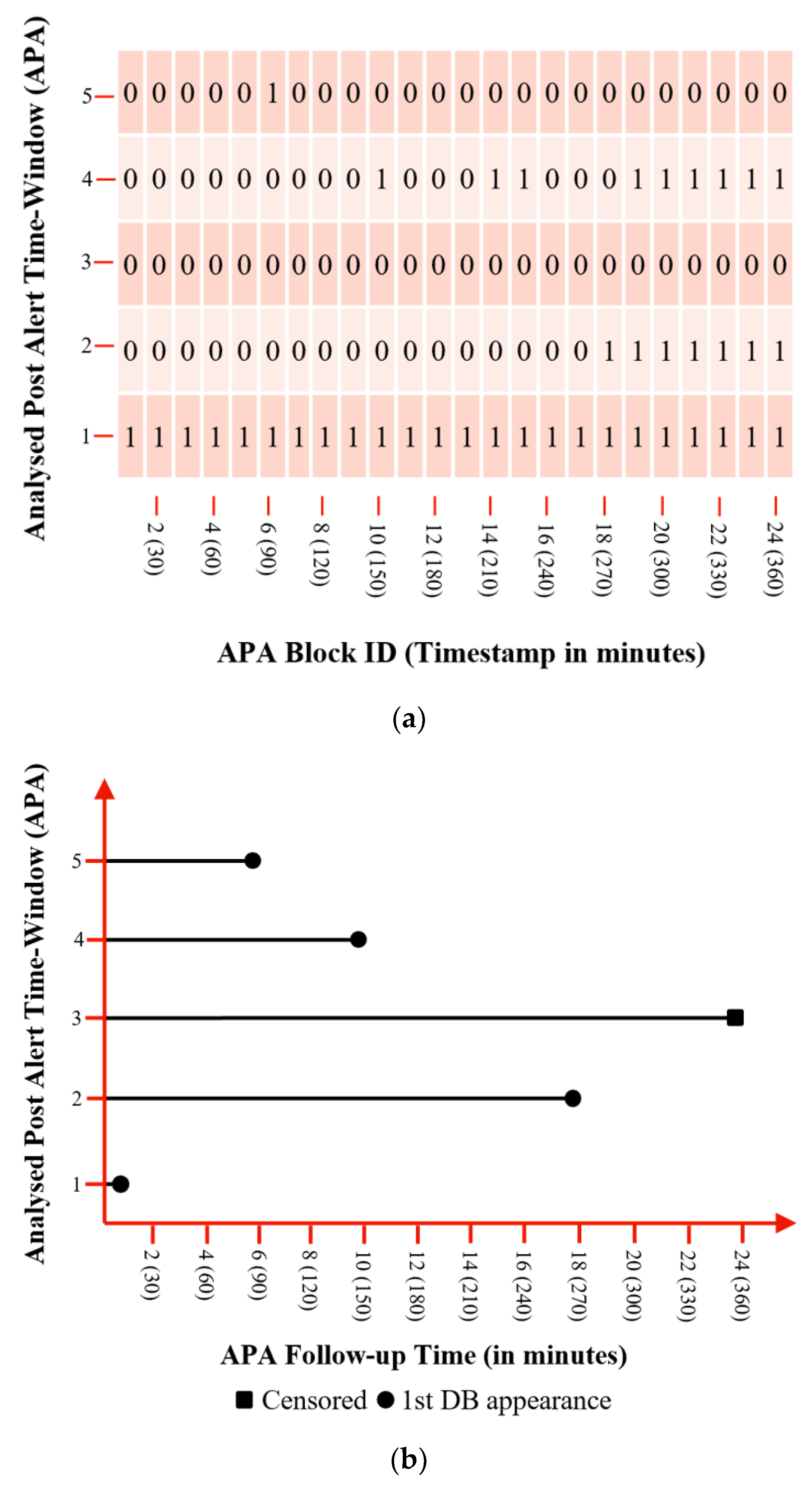
2.2. Survival Analysis Approach for Performance Estimation and Quality of Mechanical Ventilation Evaluation

Part of the challenge of building a Healthcare 4.0 system and assessing its performance and use of process data is that it relies heavily on the validation of clinicians who do not have time to exhaustively check every instance of an alarm to indicate whether it is genuine or not. This paper overcomes the need for such a laborious process by determining if the generated alerts are genuine or not by focusing on the data for the first six hours of time after the alert generation has occurred. We denote the time window, as APA (Analysed Post Alert Time-Window) and slice it into 24 consecutive blocks of 15 min time intervals. As previously mentioned, the alert is raised if TV15 is greater than 8 mL/kg for four consecutive 15 min blocks. We follow this convention based on the knowledge of when previous studies of this nature were conducted, where the data is obtained at a sampling frequency of 1 tidal volume reading per hour. The sampling frequency for the example in this paper is one reading per minute and thus waiting for four consecutive average 15 min intervals is the same as obtaining one hour’s worth of data, hence in keeping with common clinical practice [18].
We add the assumption that if TV15 is above 8 mL/kg for 4 blocks, the TV15 is expected to remain above 8 mL/kg throughout all 24 blocks of APA and such blocks are referred to as “non-defective blocks” (NDB) as these are the genuine times when we expect the patient at risk of VILI and when the alerts should be triggered. If they do not follow these criteria, then they are referred to as “defective blocks” (DB) as these are the times when the alerts are not considered genuine as the patient should indeed be receiving mechanical ventilation and there is no risk of the patient experiencing VILI. The ideal situation is to have the APA corresponding to a genuine alert that consists of only NDB. There are however many external factors that can influence the effect of mechanical ventilation such as the clinicians making a change to the patient’s treatment or a change occurring between control and support modes of the VILIAlert system. With the 24 blocks collectively making up six hours of time, it is possible that external factors can have an impact on the TV15 values and result in lower than 8 mL/kg scores, which would result in having DBs occurring during the APA.
The coding of the data from continuous TV15 readings to a discrete variable in binary form, opens up the opportunity to consider the implementation of survival analysis on the data to estimate the performance of the VILIAlert system. Survival analysis is an approach found in the statistical literature most commonly used to model time until an event occurs (survival time). As the name suggests, the original use of survival analysis was in medical research, where it was used to consider for example the event of interest for patients recovering from a disease. The time until an event occurs is known as survival time and on visual representation would typically be skewed in nature with graphs for survival times generally showing a high peak at the beginning before a long tail to the right, as fewer people experience the event as time progresses. Survival analysis is also known to accommodate the scenario of censoring when the event of interest may not have been observed for some of the individuals in the study. In such situations, survival analysis considers all the information known up to the time when censoring occurs [20].
In the context of the VILIAlert system, the event of interest is the occurrence of the DB and our aim is to predict the survival time at the point (i.e., at which APA block position) when the TV15 metric is going to drop to below 8 mL/kg upon alert generation. Therefore, the time to event is the position of the first APA block, which is marked as DB, with the longer times to event indicating better performance of the alerting algorithm. The genuine alerts will be those cases where all APA blocks are marked as NDBs and considered censored. It is important to highlight that although from the performance analytics perspective the longer follow-up times indicate better performance of the alerting algorithm, for the patient it means poorer quality of mechanical ventilation due to longer exposure of the patient to high tidal volumes, thus increasing their risk of VILI.
The raw VILIAlert data is initially analysed using the very established Kaplan–Meier (KM) method [21] to estimate the overall survival function. Let D F S ( t ) denote the overall defect free survival probability at timestamp t , i.e., the probability that the APA consists of NDB blocks only (i.e., having T V 15 > 8   mL / kg) for up to at least the time of interest t , where t = i × 15   min , and 1 i 24 is the position of the block in APA. Using the KM method this probability is estimated as follows:
D F S ^ ( t ) = n : t n t ( 1 d ( t n ) r ( t n ) ) ,
where d ( t n ) denotes the number of APA with DB event occurrence at time t n and r ( t n ) denotes the number of APA at risk prior to time t n (i.e., the number of APA that are not censored nor containing DB prior to time t n ).
The influence of other factors, the covariates, and their influence on the estimated survival curves can also be investigated using KM methods. Previous studies reported that female patients are under increased risk of receiving poorer ventilatory treatments in comparison to males [22], hence the introduced KM approach can be used to investigate the performance of the VILIAlert system in terms of these covariates. Gender can be investigated using the KM methods where each gender is considered separately, and the separate survival distributions compared for significant differences. The log-rank test may then be used to test for statistical significance of the difference in survival distributions. The results will provide information to help understand how, if at all, the patient gender is associated with the risk of receiving injurious ventilation associated with VILI and if this is an increased risk.
The KM approach described above can be seen as a static prediction as the overall survival estimates are made using the time of diagnosis (the time of generating the alert from the baseline reference) but it is unable to precisely capture how the prognosis changes over time [23]. In order to overcome this issue and process mine the changing defect free survival likelihood with increasing duration of follow-up after triggering the alert, we use the conditional survival function. This estimates the probability that APA will remain defect free until at least the time of interest t y given that it was previously defect free until the time t x , where t x < t y . In the text to follow, we will refer to this probability as the conditional defect free survival probability (CDFS), estimated using the previously described KM survival estimates (1), as follows [24,25]:
C D F S ( t y | t x ) ^ = D F S ( t y ) D F S ( t x ) ^ ^   .
The Greenwood method can be used to calculate the 95% confidence intervals (95% CI) around the CDFS estimates [24,26,27]:
95 %   C I = C D F S ( t y | t x ) ^ exp ( ± 1.96 V ^ [ log ( C D F S ( t y | t x ) ) ^ ] ) ,
where
V ^ [ log ( C D F S ( t y | t x ) ) ^ ] = 1 log ( C D F S ( t y | t x ) ^ ) k : x t k y d k r k ( r k d k )   .
Similar to the DFS, the use of the KM approach to estimate the CDFS allows us to analyse the effect of the gender covariate on the conditional survival probabilities. As the measure of effect size of conditional defect free survival differs, we use the standardised difference ( d F M ) method by Cucchetti and co-workers [28] for our study defined as:
d F M = P F P M [ P ( 1 P ) ] ,
where P F and P M are the C D F S ( t y | t x ) ^ of the female and male patients, respectively, while P represents their weighted mean [29]. To interpret the d F M values, the following guidelines are used from the literature [28,30,31]:
  • | d F M | < 0.1 
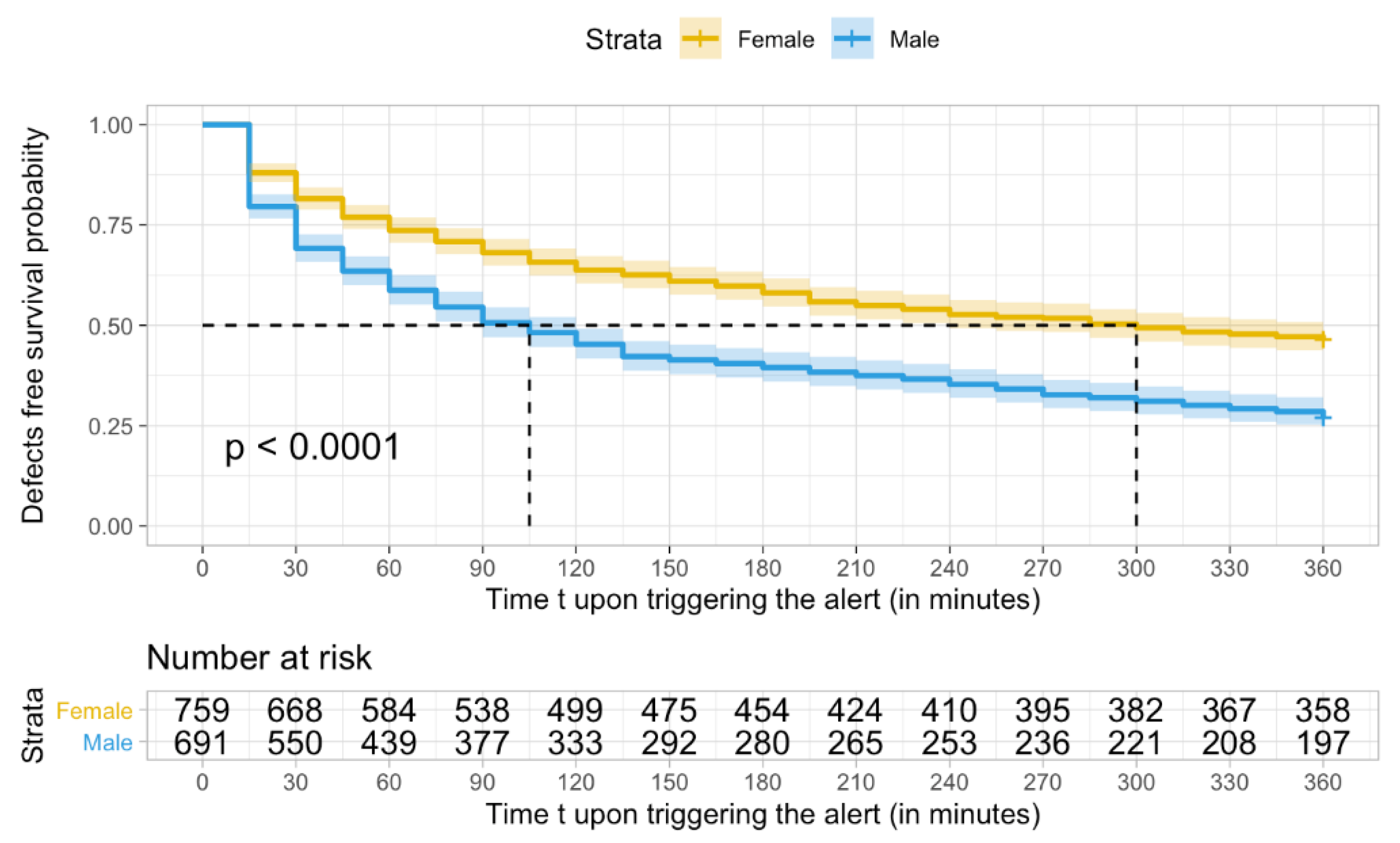
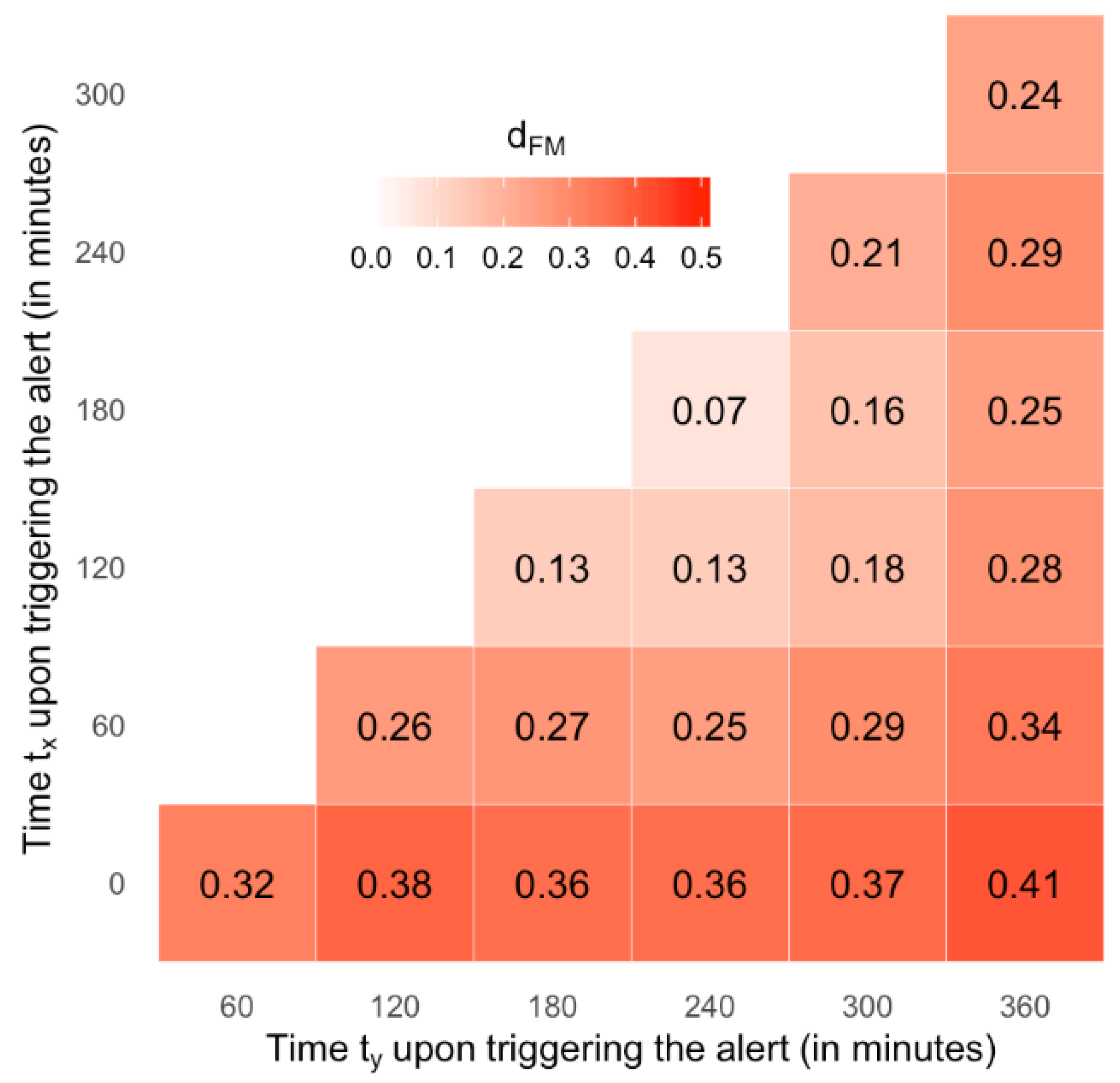
suggests very small differences;
  • 0.1 | d F M | < 0.3 suggests small differences;
  • 0.3 | d F M | < 0.5 suggests moderate differences, and;
  • 0.5 | d F M | suggests considerable differences between the two genders.
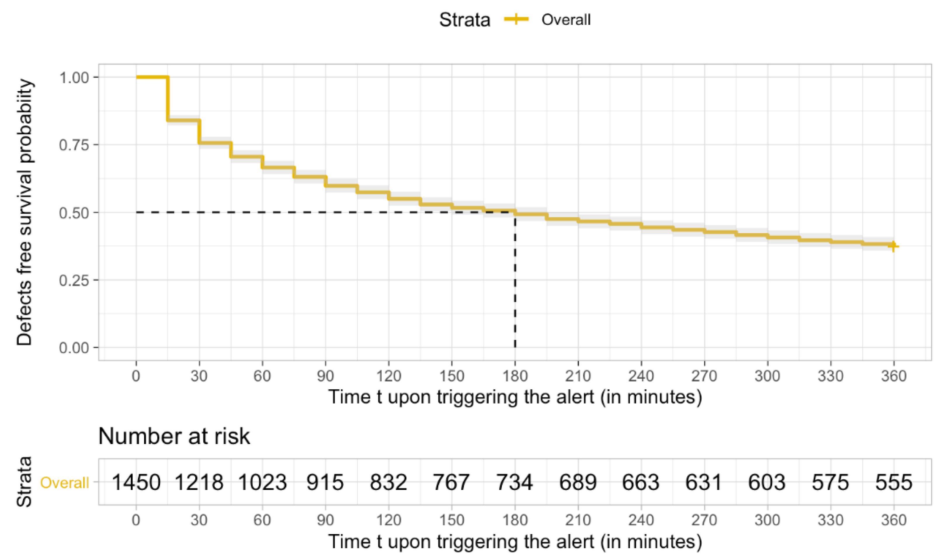
The use of survival analytics techniques for performance estimation is best illustrated with the following use-case scenario.
Figure 2a portrays an overview of the tabular dataset, in its raw form, which corresponds to 5 hypothetical APA having a length of 360 min each. Each row in this tabular dataset represents one APA segregated into 24 blocks, with each block denoting one 15 min interval over which the T V 15 values are calculated. Each block can be denoted with either 0 or 1 depending on whether it represents NDB (i.e., T V 15 > 8   mL / kg) or DB (i.e., T V 15 8   mL   /kg), respectively.
Assuming that the time to the event occurrence in APA is defined by the position of the first block, which is marked as defective (DB), we can see that the lengths of the follow-up time for the 1st, 2nd, 4th, and 5th APA are 15, 270, 150, and 90 min, respectively (illustrated in Figure 2b). As defined earlier, the remaining 3rd APA belongs to a genuine alert as it consists of NDB blocks only, and using survival analysis terminology, represents a censored event. Using Equations (1) and (2) the DFS and CDFS estimations at any time of interest t are a straightforward process, where t = i × 15   min , and 1 i 24 is the position of the block in APA. For instance, using the example above, the probability that the APA will remain defect free until the end of the follow-up period of 360 min, given that it was previously defect free during the first 90 min, can be estimated using Equation (2) as follows:
C D F S ( 360   min   | 90   min ) ^ = D F S ( 360   min ) ^ D F S ( 90   min ) ^ = 0.2 0.6 = 0.33 ,
where D F S ( 360   min ) and D F S ( 90   min ) are estimated using Equation (1). In a similar manner, using Equation (3), the CDFS 95% CI is estimated as [0.01, 0.79].
The statistical data analytics used in this paper was performed using the R v3.5.0 programming language [32] with the survival and conditional survival models being implemented using R’s survival library [33,34].

3. Results

There were 560 patients generating a total of 1450 alerts during the time in which the VILIAlert system was observed for this study. Out of the 560 patients, 298 (53%) were male patients generating 691 of the 1450 alerts (47.7%). The chi-square test of independence ( χ 2 ) and Cramér’s V ( V ) effect size coefficient indicate the existence of a strong association between the gender and alert invocation ( χ 1 2 = 42.71 ;   p = 0 ;   V = 0.22 ). This suggests that even though there were a higher proportion of males in the study, the female patients are the ones who have a higher chance of triggering the alert upon starting mechanical ventilation. An overview of the patient demographics of those involved in our VILIAlert study is provided in our earlier work [6].
In general, survival times are highly skewed and therefore best represented using the median. The time to first DB follows this skewed nature, thus it is the median overall time which is used to report time to the first DB block appearing in the APA (i.e., the median of overall defect free survival time). This is 180 min. The corresponding KM estimates are provided in Figure 3. which illustrates the estimated DFS curve for the VILIAlert data for the time until the first DB for each patient. This is typical of the survival curve shape where it is highly skewed in nature with the majority of patients experiencing the event quickly, but some taking much longer to experience the event, hence featuring in the tails of the distribution. It can be seen from Figure 3. that the probability of APA remaining defect free, i.e., the probability that T V 15 will remain above 8 mL/kg until the end of the 6 h follow-up period, decreased over time, from 0.67 at the 60th minute to 0.37 at the 360th minute upon triggering the alert.
On the other hand, the probability of the APA continuing to be defect free, conditional on it already having existed defect free in a specific time period, gradually increases. That is to say, the estimated CDFS of APA being defect free at the end of the 6 h follow-up period was more than twice lower for alerts than that which were just triggered, compared to the alerts for which their APAs were defect free for 2 h (Table 1). For instance, if APA was defect free at 60 min, the probability of it remaining defect free at the end of the follow-up period is 0.56 whereas if APA was defect free at 300 min upon triggering the alert, the probability of remaining defect free at the end of the follow-up period, from generating the alert is 0.92. A detailed overview of estimated the C D F S ( t y | t x ) probabilities for the various combinations of t x and t y timestamps in minutes, is provided in Table 1.
The median survival times for male and female patients were 105 and 300 min, respectively. Their corresponding KM estimated defect free survival curves, in Figure 4, illustrate the first DB blocks in the APAs of the males occurring much sooner during their length of stay in ICU than the female patients. The log-rank test is conducted to test whether there is a significant difference between survival times for males and females. This indicates a very highly significant difference between the male and female survival distributions ( χ 1 2 = 65.8 ,     p < 0.0001 ). The estimated DFS for male patients decreased at faster rates compared to female patients, with estimated probabilities being in the range between 0.27 and 0.59 for the male patients compared to 0.47–0.74 for the female patients in the period between 60 and 360 min from triggering the alert (Table 2). As can be seen in Figure 5 during this follow-up period ( t x = 0 ,   t y = [ 60 ,   360 ] ), the previously introduced d F M metric classifies these differences as moderate ( d F M = [ 0.32 ,   0.41 ] ) .
Similar to the overall representation, the gender stratified C D F S ^ of APA being defect free until the end of the 6 h follow-up period gradually increases for both male and female patients as APA continues to be defect free upon triggering the alert and, as shown in the Figure 6 the C D F S ^ of female patients were constantly higher than those for the males. However, results have also shown that with increased defect free survivals, the gender covariate has less effect on the conditional probabilities (Figure 5). For example, the C D F S ^ of APA being defect free at the end of the 360 min follow-up period after being previously defect free for 60, 120, 180, 240, and 300 min upon triggering the alert, were 0.63, 0.73, 0.8, 0.88, and 0.94 for female versus 0.46, 0.6, 0.69, 0.77, and 0.87 for male patients (Figure 6f) and Table 2), respectively. As shown in Figure 5, with increased defect free survivorship the differences between the genders decrease from moderate to small ( d F M = [ 0.34 ,   0.24 ] ).
A complete overview of the C D F S ^ stratified by gender and discretised by 60 min intervals is provided in Table 2, while their distribution is illustrated in Figure 6. An overview of their corresponding standardised differences ( d F M ) is illustrated in Figure 5.

4. Discussion

In this paper we presented a novel approach for analysing the performance of smart alerting real-time Healthcare 4.0 systems for scenarios in which there is no prior information that could indicate authenticity of the generated alert. The introduced technique is not a summary statistic, like for example AUC, Precision/Recall or RMSE are, where the quality of alerting algorithm is reported as a single number. Instead, the proposed approach enables researchers to dynamically estimate the probabilities that will describe for how long the patient physiological parameters exceed a certain threshold during the APA, and suggests that longer survival times indicate a better algorithm performance.
In particular, in the VILIAlert use case scenario, we hypothesised that if the alert was generated when the metric T V 15 > 8 mL/kg for four consecutive 15 min intervals, then this metric should continue to be above this threshold until the end of the 6 h long APA follow-up period. Hence the motivation for the research presented in this paper, is to model the time until the T V 15 signal drops below 8 mL/kg (which we associate the clinical activity that results in stabilisation of the patient’s health) using survival analysis methods.
The technique presented in this paper is an enhancement of our previous work [19] in which we used the KM method in collaboration with the shared-frailty time to event methods (SF) to model this phenomenon. The best resulting model was the lognormal shared-frailty model, which had patients’ height as a covariate. This showed that shorter patients are under increased risk of receiving poorer ventilation treatments, as the overall defect free probability of survival was reduced by a factor of 0.058 for each centimetre of increment in height. The motivation for an improvement from this previous work lies in the fact that both of these techniques (KM and SF) estimate the probability that T V 15 is going to stay at a value above 8 mL/kg threshold until at least the time t in APA (i.e., defect free survival probability) using the time of generating the alert as a baseline reference. Hence, previously, it was unable to dynamically predict the changing defect free survival likelihood with increasing duration of follow-up after triggering the alert. In this paper we address this issue by complementing the KM approach with the conditional survival function, which is able to estimate the probability that APA will continue to be defect free (i.e., probability that T V 15 > 8 mL/kg) until at least the time of interest t y given that it was previously defect free until the time t x , where t x < t y .
Using this technique, we compared the quality of the alerts generated by the system for the two genders, and discovered that the alerting algorithm had better performance in the female patients compared to the male patients. This is according to the higher defect free and conditional defect free survival probabilities. However, it is important to put this into the survival time context. The median survival times for females is almost three times longer than that for male patients, which would actually suggest that the female patients receive poorer ventilation treatment than male patients due to them being exposed to the higher risk of injuriously high TVs (>8 mL/kg) for a much longer period of time, thus having a higher risk of developing VILI. The longer that patients remain on the ventilator event free, the more potential there is for damage, which could be construed as the lesser quality of care. In addition to our earlier findings [19], the results presented in this paper have confirmed that they are consistent with discoveries from the literature, which suggests that the female patients, as well as those patients who in general are a shorter height, receive poorer quality of mechanical ventilation treatments. In particular, previous findings have shown that the female patients and whose height is of less than 165 cm are at an increased risk of receiving injurious ventilation [22].
Despite getting increased popularity in healthcare [35,36,37,38,39,40], to our knowledge this is the first time the technique presented in this paper has been used for dynamic modelling of the performance of real-time Healthcare 4.0 alerting systems, as well as for the indirect evaluation of the quality of received care.
The approach introduced and demonstrated in this paper could be implemented during the development of any new algorithm in this setting, allowing for a comparison to be made across many algorithms. In evaluating the performance of the VILIAlert system, we provided a framework (guidelines) that is applicable to any real-time system capturing non-labelled data, not just the use case included for illustration purposes in this paper. Indeed, the approach could be used for developing a better understanding of the systems behaviour in addition to the new algorithm development and the cross comparison of algorithm performances for use in areas such as biosensor driven healthcare monitoring [41,42].

5. Conclusions

In this paper we have introduced a novel process mining technique based on the principles of survival and conditional survival analysis for estimating the performance and the evaluation of the quality of care of real-time Healthcare 4.0 systems. The approach has been successfully demonstrated using a real-time system that receives data flows from ventilators in a hospital setting. The work has also highlighted further developments that can be considered using recurrent survival analysis and the incorporation of further visual data analytics into the approaches.

Author Contributions

Conceptualization, A.H.M. and A.N.; Methodology, A.H.M. and A.N.; Software, A.N.; Validation, A.H.M.; Visualization, A.N.; Writing—original draft, A.N.; Writing—review & editing, A.H.M. All authors have read and agreed to the published version of the manuscript.

Funding

This research has been funded by Queen’s University Belfast, United Kingdom.

Institutional Review Board Statement

Not applicable.

Informed Consent Statement

Patient consent was waived due to this work being carried out as part of an ongoing Quality Improvement Project to improve the quality of mechanical ventilation in the Regional Intensive Care Unit, Royal Victoria Hospital, Belfast. Routinely collected anonymised data is used to develop the VILIAlert system. Ethical approval was deemed unnecessary by the research governance department of the Belfast Health and Social Care Trust.

Data Availability Statement

The anonymised data set for this study is held securely at Queen’s University Belfast. Data sharing regulations prevent this data from being made available publicly.

Acknowledgments

The authors wish to acknowledge the Royal Victoria Hospital for facilitating the testing and validation of the VILIAlert system. We would also like to thank Charles J Gillan (Institute of Electr onics, Communications and Information Technology) and Murali Shyamsundar (The Centre for Experimental Medicine, School of Medicine Dentistry and Biological Sciences) from Queen’s University Belfast.

Conflicts of Interest

The authors declare no conflict of interest.

Abbreviations

APAAnalysed Post Alert Time Window
AUCArea Under the receiver operator characteristic Curve
CDFSConditional Defect Free Survival probability
CDSClinical Decision Support System
CIConfidence Interval
DBDefective Blocks
DFSDefect Free Survival probability
EMRElectronic Medical Record
HL7Health Level 7
IBWIdeal Body Weight
ICUIntensive Care Unit
KMKaplan-Meier
LPVLung Protective Ventilation
NDBNon-Defective Blocks
RMSERoot Mean Square Error
SFShared Frailty
SPCStatistical Process Control
TVTidal Volume in ml/inspiration units
TV15Averaged TV values, calculated over 15 min time intervals
VILIVentilator Induced Lung Injury

References

  1. Rojas, E.; Munoz-Gama, J.; Sepúlveda, M.; Capurro, D. Process mining in healthcare: A literature review. J. Biomed. Inform. 2016, 61, 224–236. [Google Scholar] [CrossRef]
  2. Plathong, K.; Surakratanasakul, B. A study of integration Internet of Things with health level 7 protocol for real-time healthcare monitoring by using cloud computing. In Proceedings of the 10th Biomedical Engineering International Conference (BMEiCON), Hokkaido, Japan, 31 August–2 September 2017. [Google Scholar]
  3. Health Level Seven International. About HL7. Available online: https://bit.ly/2tkavDk (accessed on 5 February 2019).
  4. Zhang, J.; Xu, W.; Guo, J.; Gao, S. A temporal model in electronic health record search. Knowl.-Based Syst. 2017, 126, 56–67. [Google Scholar] [CrossRef]
  5. Amato, F.; de Pietro, G.; Esposito, M.; Mazzocca, N. An integrated framework for securing semi-structural health records. Knowl.-Based Syst. 2015, 79, 99–117. [Google Scholar] [CrossRef]
  6. Novakovic, A.; Marshall, A.H. Introducing the DM-P approach for analysing the performances of real-time clinical decision support systems. Knowl.-Based Syst. 2020, 198, 105877. [Google Scholar] [CrossRef]
  7. Ghassemi, M.; Celi, L.A.; Stone, D.J. State of the art review: The data revolution in critical care. Crit. Care 2015, 19, 118. [Google Scholar] [CrossRef] [Green Version]
  8. Slutsky, A.S.; Ranieri, V.M. Ventilator-Induced Lung Injury. N. Engl. J. Med. 2013, 369, 2126–2136. [Google Scholar] [CrossRef] [Green Version]
  9. Determann, R.M.; Royakkers, A.; Wolthuis, E.K.; Vlaar, A.P.; Choi, G.; Paulus, F.; Hofstra, J.J.; de Graaff, M.J.; Korevaar, J.C.; Schultz, M.J. Ventilation with lower tidal volumes as compared with conventional tidal volumes for patients without acute lung injury: A preventive randomized controlled trial. Crit. Care 2010, 14, R1. [Google Scholar] [CrossRef] [Green Version]
  10. Amato, M.B.P.; Barbas, C.S.V.; Medeiros, D.M.; Magaldi, R.B.; Schettino, G.P.; Lorenzi-Filho, G.; Kairalla, R.A.; Deheinzelin, D.; Munoz, C.; Oliveira, R.; et al. Effect of a protective-ventilation strategy on mortality in the acute respiratory distress syndrome. N. Engl. J. Med. 1998, 338, 347–354. [Google Scholar] [CrossRef]
  11. Putensen, C.; Theuerkauf, N.; Zinserling, J.; Wrigge, H.; Pelosi, P. Meta-analysis: Ventilation strategies and outcomes of the acute respiratory distress syndrome and acute lung injury. Ann. Intern. Med. 2009, 151, 566–576. [Google Scholar] [CrossRef]
  12. Neto, A.S. Lung-Protective Ventilation in Intensive Care Unit and Operation Room: Tidal Volume Size, Level of Positive End-Expiratory Pressure and Driving Pressure; Faculty of Medicine, University of Amsterdam: Amsterdam, The Netherlands, 2017; Available online: https://dare.uva.nl/search?identifier=35660734-9d32-4127-8608-68207d9d5d28 (accessed on 1 April 2022).
  13. Walkey, A.J.; Wiener, R.S. Risk Factors for Underuse of Lung Protective Ventilation in Acute Lung Injury. Crit. Care 2012, 27, 323.e1–323.e9. [Google Scholar] [CrossRef] [Green Version]
  14. Checkley, W.; Brower, R.; Korpak, A.; Thompson, B.T. Effects of a clinical trial on mechanical ventilation practices in patients with acute lung injury. Am. J. Respir. Crit. Care Med. 2008, 177, 1215–1222. [Google Scholar] [CrossRef] [PubMed]
  15. Kalhan, R.; Mikkelsen, M.; Dedhiya, P.; Christie, J.; Gaughan, C.; Lanken, P.N.; Finkel, B.; Gallop, R.; Fuchs, B.D. Underuse of lung protective ventilation: Analysis of potential factors to explain physician behavior. Crit. Care Med. 2006, 34, 300–306. [Google Scholar] [CrossRef]
  16. Gillan, C.J.; Novakovic, A.; Marshall, A.H.; Shyamsundar, M.; Nikolopoulos, D.S. Expediting assessments of database performance for streams of respiratory parameters. Comput. Biol. Med. 2018, 100, 186–195. [Google Scholar] [CrossRef] [Green Version]
  17. Herasevich, V.; Tsapenko, M.; Kojicic, M.; Ahmed, A.; Kashyap, R.; Venkata, C.; Shahjehan, K.; Thakur, S.J.; Pickering, B.W.; Zhang, J.; et al. Limiting ventilator-induced lung injury through individual electronic medical record surveillance. Crit. Care Med. 2011, 39, 34–39. [Google Scholar] [CrossRef]
  18. Bourdeaux, C.P.; Thomas, M.J.; Gould, T.H.; Malhotra, G.; Jarvstad, A.; Jones, T.; Gilchrist, I.D. Increasing compliance with low tidal volume ventilation in the ICU with two nudge-based interventions: Evaluation through intervention time-series analysis. BMJ Open 2016, 6, e010129. [Google Scholar] [CrossRef] [PubMed] [Green Version]
  19. Marshall, A.H.; Novakovic, A. Analysing the performance of a real-time Healthcare 4.0 system using shared frailty time to event models. In Proceedings of the 2019 IEEE 32nd International Symposium on Computer-Based Medical Systems (CBMS), Cordoba, Spain, 5–7 June 2019. [Google Scholar]
  20. Austin, P.C. A Tutorial on Multilevel Survival Analysis: Methods, Models, Applications. Int. Stat. Rev. 2017, 85, 185–203. [Google Scholar] [CrossRef]
  21. Kaplan, E.L.; Meier, P. Nonparametric estimation from incomplete observations. J. Am. Stat. Assoc. 1958, 53, 457–481. [Google Scholar] [CrossRef]
  22. Bustamante, A.F.; Wood, C.L.; Tran, Z.V.; Moine, P. Intraoperative ventilation: Incidence and risk factors for receiving large tidal volumes during general anesthesia. BMC Anesthesiol. 2011, 11, 22. [Google Scholar]
  23. Hieke, S.; Konig, C.; Engelhardt, M.; Schumacher, M. Conditional Survival: A Useful Concept to Provide Information on How Prognosis Evolves over Time. Clin. Cancer Res. 2015, 21, 1530–1536. [Google Scholar] [CrossRef] [Green Version]
  24. Jung, S.-H.; Lee, H.Y.; Chow, S.-C. Statistical Methods for Conditional Survival Analysis. J. Biopharm. Stat. 2018, 28, 927–938. [Google Scholar] [CrossRef]
  25. Zabor, E.C.; Gonen, M.; Chapman, P.B.; Panageas, K.S. Dynamic Prognostication Using Conditional Survival Estimates. Cancer 2013, 119, 3589–3592. [Google Scholar] [CrossRef]
  26. Davis, F.G.; McCarthy, B.J.; Freels, S.; Kupelian, V.; Bondy, M.L. The conditional probability of survival of patients with primary malignant brain tumors. Cancer 1999, 85, 485–491. [Google Scholar] [CrossRef]
  27. Yuan, X.; Rai, S.N. Confidence Intervals for Survival Probabilities: A Comparison Study. Commun. Stat. Simul. Comput. 2011, 40, 978–991. [Google Scholar] [CrossRef]
  28. Cucchetti, A.; Piscaglia, F.; Cescon, M.; Ercolani, G.; Terzi, E.; Bolondi, L.; Zanello, M.; Pinna, A.D. Conditional Survival after Hepatic Resection for Hepatocellular Carcinoma in Cirrhotic Patients. Clin. Cancer Res. 2012, 18, 4397–4405. [Google Scholar] [CrossRef] [PubMed] [Green Version]
  29. Burnard, B.; Kernan, W.N.; Feinstein, A.R. Indexes and boundaries for “quantitative significance” in statistical decisions. J. Clin. Epidimiol. 1990, 43, 1273–1284. [Google Scholar] [CrossRef]
  30. Kim, Y.; Margonis, G.A.; Prescott, J.D.; Tran, T.B.; Postlewait, L.M.; Maithel, S.K.; Wang, T.S.; Glenn, J.A.; Hatzaras, I.; Shenoy, R.; et al. Curative Surgical Resection of Adrenocortical Carcinoma: Determining Long-term Outcome Based on Conditional Disease-free Probability. Ann. Surg. 2017, 265, 197–204. [Google Scholar] [CrossRef] [PubMed] [Green Version]
  31. Shao, N.; Wan, F.; Abudurexiti, M.; Wang, J.; Zhu, Y.; Ye, D. Causes of Death and Conditional Survival of Renal Cell Carcinoma. Front. Oncol. 2019, 9, 591. [Google Scholar] [CrossRef] [PubMed] [Green Version]
  32. R Core Team. R: A Language and Environment for Statistical Computing; R Foundation for Statistical Computing: Vienna, Austria, 2018. [Google Scholar]
  33. Therneau, T.M. A Package for Survival Analysis in S. 2015. Available online: https://CRAN.R-project.org/package=survival (accessed on 1 April 2022).
  34. Thernau, T.M.; Grambsch, P.M. Modeling Survival Data: Extending the Cox Model; Springer: New York, NY, USA, 2000. [Google Scholar]
  35. Kang, M.; Kim, H.S.; Jeong, C.W.; Kwak, C.; Kim, H.H.; Ku, J.H. Prognostic factors for conditional survival in patients with muscle-invasive urothelial carcinoma of the bladder treated with radical cystectomy. Sci. Rep. 2015, 5, 12171. [Google Scholar] [CrossRef] [Green Version]
  36. Bischof, D.A.; Kim, Y.; Dodson, R.; Jimenez, M.C.; Behman, R.; Cocieru, A.; Fisher, S.B.; Groeschl, R.T.; Squires, M.H.; Maithel, S.K.; et al. Conditional Disease-Free Survival After Surgical Resection of Gastrointestinal Stromal Tumors: A Multi-institutional Analysis of 502 Patients. JAMA Surg. 2015, 150, 299–306. [Google Scholar] [CrossRef] [Green Version]
  37. Multidisciplinary Larynx Cancer Working Group; Sheu, T.; Vock, D.M.; Mohamed, A.S.R.; Gross, N.; Mulcahy, C.; Zafereo, M.; Gunn, G.B.; Garden, A.; Sevak, P.; et al. Conditional Survival Analysis of Patients with Locally Advanced Laryngeal Cancer: Construction of a Dynamic Risk Model and Clinical Nomogram. Sci. Rep. 2017, 7, 43928. [Google Scholar]
  38. Kang, M.; Park, J.Y.; Jeong, C.W.; Hwang, E.C.; Song, C.; Hong, S.H.; Kwak, C.; Chung, J.; Sung, H.H.; Jeon, H.G.; et al. Changeable Conditional Survival Rates and Associated Prognosticators in Patients with Metastatic Renal Cell Carcinoma Receiving First Line Targeted Therapy. J. Urol. 2018, 200, 989–995. [Google Scholar] [CrossRef]
  39. Liu, X.; Wu, T.; Zhu, S.Y.; Shi, M.; Su, H.; Wang, Y.; He, X.; Xu, L.-M.; Yuan, Z.-Y.; Zhang, L.-L.; et al. Risk-Dependent Conditional Survival and Failure Hazard After Radiotherapy for Early-Stage Extranodal Natural Killer/T-Cell Lymphoma. JAMA Netw. Open 2019, 2, e190194. [Google Scholar] [CrossRef] [PubMed]
  40. Narita, S.; Nomura, K.; Hatakeyama, S.; Takahashi, M.; Sakurai, T.; Kawamura, S.; Hoshi, S.; Ishida, M.; Kawaguchi, T.; Ishidoya, S.; et al. Changes in conditional net survival and dynamic prognostic factors in patients with newly diagnosed metastatic prostate cancer initially treated with androgen deprivation therapy. Cancer Med. 2019, 8, 6566–6577. [Google Scholar] [CrossRef] [PubMed]
  41. Luo, Y.; Cai, J.; Huang, Y.; Luo, J. Ultra-sensitive DNAzyme-based optofluidic biosensor with liquid crystal-Au nanoparticle hybrid amplification for molecular detection. Sens. Actuators B Chem. 2022, 359, 131608. [Google Scholar]
  42. Zahed, M.A.; Yoon, H.; Sharifuzzaman, M.; Yoon, S.H.; Kim, D.K.; Do Shin, Y.; Asaduzzaman, M.; Park, J.Y. Nanoporous Carbon-Based Wearable Hybrid Biosensing Patch for Real-Time and in Vitro Healthcare Monitoring. In Proceedings of the 2022 IEEE 35th International Conference on Micro Electro Mechanical Systems Conference (MEMS), Tokyo, Japan, 9–13 January 2022. [Google Scholar]
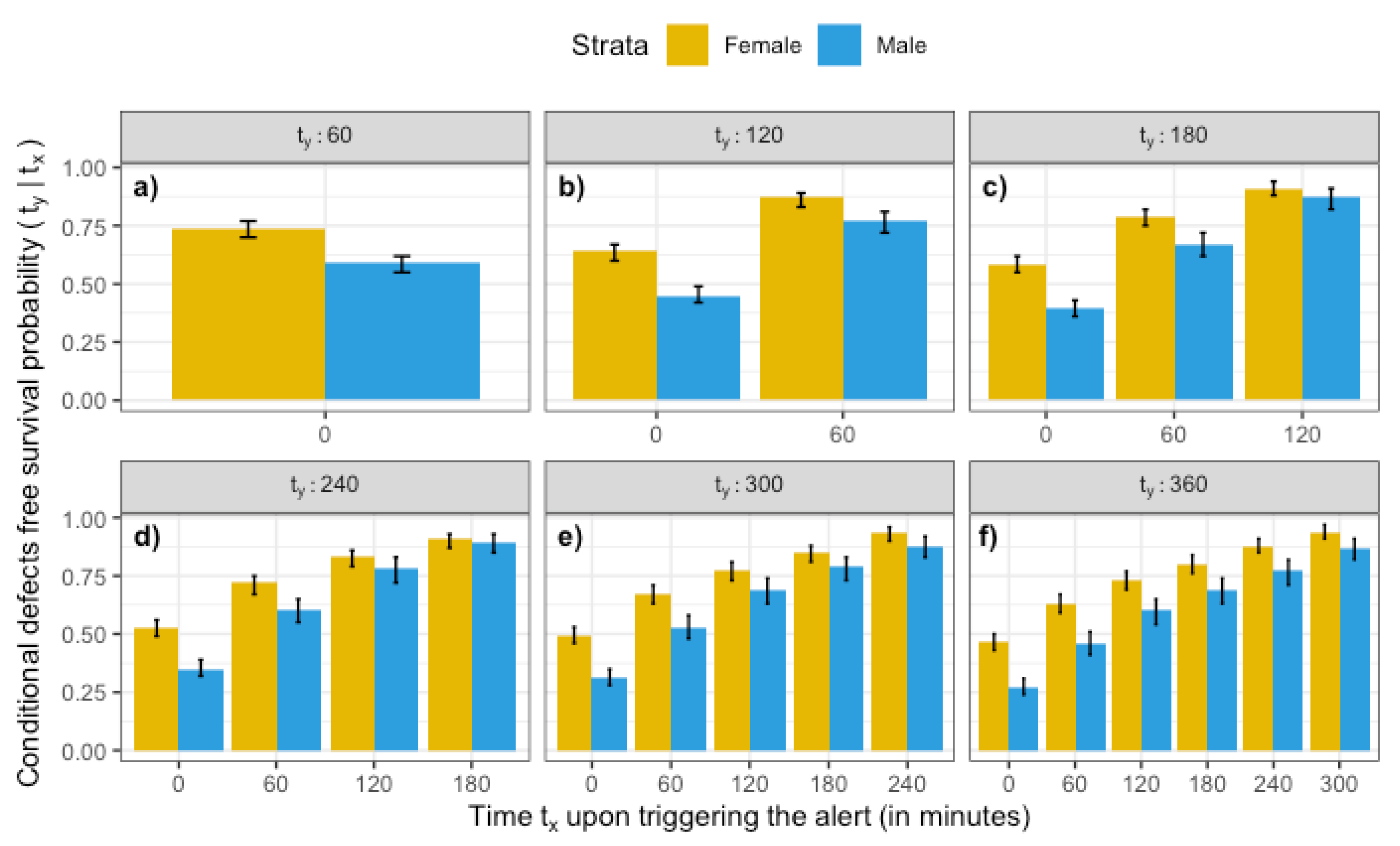
Figure 1. An architectural overview of the VILIAlert System [19].
Algorithms 15 00196 g001
Figure 2. A schematic overview of five analysed post alert time windows (APA) covering the period of 6 h post-alert generation. (a) An illustration of the tabular dataset in its raw form, where 0 and 1 symbolise defective (DB) and non-defective (NDB) blocks, respectively. (b) An illustration of the lengths of their follow-up times, where each length corresponds to the time to occurrence of the event of interest, i.e., 1st DB block during APA. These lengths are used for the calculation of defect free and conditional defect free survival probabilities.
Algorithms 15 00196 g002
Figure 3. Kaplan–Meier estimates of overall defect free survival probability.
Algorithms 15 00196 g003
Figure 4. Kaplan–Meier estimates of gender stratified overall defect free survival probability.
Algorithms 15 00196 g004
Figure 5. An overview of standardised differences ( d F M ) used for analysing the effect size that the gender covariate has estimated the conditional defect free survival probabilities C D F S   ( t y | t x ) . Note: t x = 0 denotes baseline time, i.e., the time of alert generation.
Algorithms 15 00196 g005
Figure 6. An overview of conditional defect free survival probabilities (including their 95% confidence intervals) denoting that analysed post alert time window will remain defect free until at least time t y given that it was previously defect free to the time t x , where t x < t y . Note: t x = 0 denotes baseline time, i.e., the time of alert generation.
Algorithms 15 00196 g006
Table 1. An overview of estimated overall conditional defect free survival probabilities, and their corresponding 95% confidence intervals (CI), to various timestamps in minutes t y , conditioned on APA being defect free until timestamps t x upon triggering the alert. Note: t x = 0 denotes the baseline time, i.e., the time of alert generation.
C D F S   ( t y | t x ) ^   ( 95 %   CI )
t y 60120180240300360
t x
Overall
(1450 alerts)
00.67
(0.64, 0.69)
0.55
(0.52, 0.57)
0.49
(0.47, 0.52)
0.44
(0.42, 0.47)
0.41
(0.38, 0.43)
0.37
(0.35, 0.4)
600.83
(0.8, 0.85)
0.74
(0.71, 0.77)
0.67
(0.63, 0.7)
0.61
(0.58, 0.64)
0.56
(0.53, 0.59)
1200.9
(0.87, 0.92)
0.81
(0.78, 0.84)
0.74
(0.71, 0.77)
0.68
(0.64, 0.71)
1800.9
(0.87, 0.92)
0.83
(0.79, 0.85)
0.76
(0.72, 0.79)
2400.92
(0.89, 0.94)
0.84
(0.81, 0.87)
3000.92
(0.89, 0.94)
Table 2. An overview of the estimated conditional defect free survival probabilities stratified by gender, and their corresponding 95% confidence intervals (CI) to various timestamps in minutes t y , conditional onAPA being defect free until timestamps t x upon triggering the alert. Note: t x = 0 denotes baseline time, i.e., the time of alert generation.
C D F S ( t y | t x ) ^   ( 95 %   CI )
t y 60120180240300360
t x
Female
(759 alerts)
00.74
(0.7, 0.77)
0.64
(0.6, 0.67)
0.58 (0.55, 0.62)0.53
(0.49, 0.56)
0.49
(0.46, 0.53)
0.47
(0.43, 0.5)
600.87
(0.83, 0.89)
0.79
(0.75, 0.82)
0.72
(0.67, 0.75)
0.67
(0.63, 0.71)
0.63
(0.59, 0.67)
1200.91
(0.88, 0.94)
0.83
(0.79, 0.86)
0.77
(0.73, 0.81)
0.73
(0.69, 0.77)
1800.91
(0.87, 0.93)
0.85
(0.81, 0.88)
0.8
(0.76, 0.84)
2400.94
(0.9, 0.96)
0.88
(0.85, 0.91)
3000.94
(0.91, 0.97)
Male
(691 alerts)
00.59 (0.55, 0.62)0.45
(0.42, 0.49)
0.4
(0.36, 0.43)
0.35
(0.32, 0.39)
0.31
(0.28, 0.35)
0.27
(0.24, 0.31)
600.77
(0.72, 0.81)
0.67
(0.62, 0.72)
0.6
(0.55, 0.65)
0.53
(0.48, 0.58)
0.46
(0.41, 0.51)
1200.87
(0.82, 0.91)
0.78
(0.72, 0.83)
0.69
(0.63, 0.74)
0.6
0(.54, 0.65)
1800.89
(0.85, 0.93)
0.79
(0.73, 0.83)
0.69
(0.63, 0.74)
2400.88
(0.83, 0.92)
0.77
(0.71, 0.82)
3000.87
(0.82, 0.91)
Publisher’s Note: MDPI stays neutral with regard to jurisdictional claims in published maps and institutional affiliations.

