A Multi-Objective Model and Algorithms of Aggregate Production Planning of Multi-Product with Early and Late Delivery

Abstract

Due to the influence of insufficient production capacity or shortage of production materials, production enterprises may produce products in advance or be backordered. In order to improve the adaptability of enterprises and reduce production costs, the impacts of early delivery and delayed delivery are analyzed, and the method to determine the loss threshold is put forward. Moreover, the maximum allowable shortage of customers with different tardiness is calculated, and the cost of delayed delivery and loss of sales is determined. Considering the production cost, raw material cost, inventory cost, staff cost, stockout, and lost sales cost, an early/delay multi-objective optimization model is developed for an aggregate production planning (APP) problem to minimize total production costs and instability in the workforce. Three algorithms and three different hybrid strategies are designed to solve the model. Finally, some test experiments are employed in order to validate the performance of the proposed evaluation of the three algorithms. The results show that: The method of determining the loss threshold can effectively reflect the double influence of customer satisfaction with waiting time and shortage quantity. The definition of unit tardiness cost reflects the law that it increases gradually with waiting time. The determination of the feasible range of product output and the number of workers in the workforce can reduce the search scope of the algorithm and improve the efficiency of the algorithm.

1. Introduction

Aggregate production planning (APP) is an operational activity that determines the minimum cost, workforce, and production plans required to meet customer demands. APP simultaneously establishes optimal production, inventory, and employment levels over a given finite planning horizon to meet the total demand for all products that share the same limited resources [1]. As the implementation of JIT (Just in Time) practice becomes increasingly popular, each echelon in a supply chain tends to carry smaller inventories, and thus the whole supply chain is made more vulnerable to lost sales and/or backorders [2]. Furthermore, with the development of the manufacturing industry, more dynamic characteristics of production need to be considered in practical application. Therefore, the APP model should include multiple factors related to production and inventory, such as production cost, labor cost, inventory cost, etc. and should also consider some extension conditions, such as backorder cost, overtime cost, and lost sales cost.

APP is one of the most critical areas of planning performed in the design of production systems, and it has attracted considerable interest from both practitioners and academics [1]. Many researchers have considered the backordering decisions in the APP model. We summarized the most important and related studies that consider backordering for APP in

Table 1. The related studies considering the backordering for APP.

Article	Model Category	Objective Function	Considerations	Solving Approaches
Wang and Liang [3]	Multiple objective linear programming model	Total production costs; Carrying and backordering costs; Costs of changes in labor levels	Inventory levels; labor levels; machine capacity; warehouse space; the time value of money	Solution algorithm based on linear programming problem
Ning et al. [4]	A fuzzy random APP model	The chance of obtaining the profit more than the predetermined profit	The market demand; production cost; subcontracting cost; inventory carrying cost; backorder cost; product capacity; sales revenue; maximum labor level; maximum capital level	A hybrid optimization algorithm
Mahdavi et al. [5]	An integer mathematical programming model	The summation of machine, reconfiguration, inter-cell material handling, inventory holding, backorder, worker hiring, firing and salary costs	The available time for workers; capacity of machine; worker assignment; worker assignment	Linearized using some auxiliary variables
Chakrabortty and Hasin [6]	Multiple objective linear programming model	The production costs; the carrying and backordering cost; the rate of change in labor levels	Inventory levels; labor levels; overtime; subcontracting and backordering levels; labor, machine and warehouse capacity	Multi-Objective Genetic Algorithm
Sadeghi et al. [7]	Fuzzy Grey Goal Programming model	The total production costs; the total carrying and backordering costs; the rate of changes in workforce level	machine capacity and warehouse space; labor levels; carrying inventory	A goal programming approach
Saidi-Mehrab et al. [8]	Integer linear programming model	The total costs of machine maintenance and overhead, system reconfiguration, backorder and inventory holding, training and salaryof workers	Demand satisfaction; machineavailability; machine time-capacity; available time of worker and training	Linearized using some auxiliary variables
Basis et al. [9]	Mixed integer linear programming model	The total cost composed of production, setup, raw material supply, inventory holding and backorder penalty	Demand satisfaction; material balance; inventory capacity; the relationship between setup binary and production quantity	A rolling horizon-based approach
Modarres and Izadpanahi [10]	Linear programming model	The operational cost (including backorder and inventory carrying costs); the energy cost; carbon emission	Demand satisfaction; limits for each product in each period and total production; energy consumption	The goal attainment technique
Hossain et al. [11]	Mixed integer linear programming model	The total costs in terms of inventory levels, labor levels, overtime, subcontracting and backordering levels, and labor, machine, warehouse capacity, incentive and wastage cost	The time varying demand, unstable production capacity and work forces, inventory control, wastage reduction, and proper incentive for workforce	Genetic Algorithm Optimization approach and Big M method
Sakhaii et al. [12]	Deterministic nonlinear mathematical model	The costs of machine breakdown and relocation, operator training and hiring, inter-intra cell part trip, and shortage and inventory	The inter-cell layout, machine reliability and relocation, machine capacity and operator assignment	Linearized
Mehdizadeh et al. [13]	Multi-objective optimization model	The profit by improving learning and reducing the failure cost of the system; the costs associated with repairs and deterioration	The market demands; the machine capacity; the limitation on the total quantity produced; the workforce levels of labor groups; inventory capacity	Subpopulation genetic algorithm; weighted sum multi-objective genetic algorithm and nondominated sorting genetic algorithm II
Jamalnia et al. [14]	A framework based on a set of stochastic, nonlinear, multi-objective optimization models	The total revenue; total production costs; utilization of production resources and capacity	The production capacity; the product demand; workforce	The multiple criteria decision-making methods Additive value function, TOPSIS and VIKOR
Xue and Offodile [15]	Non-linear mixed integer programming model	The total cost of machine maintenance and overhead, inter- and intra-cell material handling, inventory holding, subcontracting, and backordering	The production-inventory balance; production consistency; the lower and upper bounds for the production level; the capacity limits; the machine balance; the storage space limits; the maximal backordering level	Linearized
Jang and Chung [16]	A robust optimization model	The total costs composed of regular time labor costs, overtime labor costs, hiring costs, layoff costs, and product-related costs that include producing, holding inventory, backlogging, and subcontracting costs	The workforce level; the production capacity; the production balance; overtime labor limit	Bi-level particleswarm optimization

.

Throughout the review, multi-objective programming has been widely used in this area, and most of the existing research on APP mainly consider the constraints on the balance equation for production, inventory capacity, inventory and demand, production capacity, and labor capacity. Moreover, the production cost, inventory and backorder level are the other main objectives that have been taken into consideration. The main methods applied to management science techniques for APP problems are: linear programming, piecewise linear programming, nonlinear programming, etc.

Table 2. The characteristics of the existing models.

Issue	Description
Product demand	Be deterministic, and must be satisfied by product, inventory, or backorder
Production costs	Strictly linear or piecewise linear in any given planning period (consist of regular time and overtime production and costs of inventory and backorders)
Inventory	Be limited over the entire planning horizon
Capacity	Inventory capacity, production capacity and labor capacity are mainly considered
Backorders	May or may not be allowed
Multiple product	In most APP models more than one product exists
Labor characteristics	Some important labor characteristics are considered in some APP models, such as labor skills, labor training, labor productivity, and constant level
Objective	The costs associated with meeting a known demand, the total revenue of the system or inventory and backorder level
Constraints	The balance equation for production, inventory capacity, inventory and demand, pro-duction capacity, and labor capacity
Model category	Linear programming, piecewise linear programming, nonlinear programming, etc.

shows some of the characteristics of the existing models.

Furthermore, Florian et al. [17] analyzed the computational complexity of a class of deterministic production planning problems with various types of cost functions and proved that the single material problem under the constraints of linear cost function and time-varying capacity and some special cases are NP-hard. Chen and Thizy [18] also proved that the multi-item capacitated production planning problem is strongly NP-hard. In addition, according to Ramezanian et al. [19] and Mehdizadeh et al. [13], APP problems with multi-phase production are among strongly NP-hard issues. Moreover, metaheuristics have proved to be efficient techniques for solving APP problems. Among the metaheuristics, genetic algorithms (GAs) (Chakrabortty et al. [6], Hossain et al. [11], Mehdizadeh et al. [13], Ramezanian et al. [19], Liu et al. [20]), and particle swarm optimization (PSO) (Jang et al. [16], Wang et al. [21], Chakrabortty et al. [22]) have been used to deal with APP models.

As a major factor determining the production capacity of enterprises, labor costs account for an increasing proportion. Therefore, decision makers pay great attention to the impact of labor changes, and the stability of workers has become more important than ever. Furthermore, the fluctuation of demand will lead to a change in enterprise employment. So, the stability of employment is extremely important to the APP problem. Therefore, in the objective function, the sum of the changes in the number of workers is used to measure its stability. In reality, due to the decline of actual production capacity caused by the change of workers, equipment maintenance or damage, holidays and sudden epidemic situations, or due to the shortage of production materials, production enterprises may produce products in advance or be backordered. Both of these situations will affect the cost of the enterprise. In order to improve the adaptability of enterprises and reduce production costs, it is necessary to properly arrange the production plan to improve the production management level of the enterprise.

In considering the situation of production in advance or backorder, this paper analyzes the impact of backorders and determines the cost of backorder and loss of sales. Furthermore, a bi-objective optimization model for an APP problem of multi-product, multi-stage with early and late delivery minimizes total production costs and instability in the workforce, considering the balance equation for production, product demand, labor, inventory and production capacity, and different worker types. In order to improve the efficiency of solving large-scale multi-objective APP problems, a local search (LS) algorithm is based on the minimum cost flow (MCF). Further, in order to improve the speed of solving APP problems, hybrid strategies based on local search-based GA (LS-GA), hybrid genetic algorithm-particle swarm optimization based on stages (HGA-PSO1) and multi-population strategy (HGA-PSO2) are adopted to solve this model. Finally, the performances of the proposed evaluation of the multi-objective algorithm are selected to compare and analyze each algorithm.

The remainder of this paper is organized as follows: Section 2.1 introduces some notations. Section 2.2 analyzes the impacts of production in advance and backorder. In Section 2.3 and Section 2.4, the objective functions and constraints are discussed, respectively. In addition, the GA and the LS algorithm based on MCF are proposed in Section 3.1 and Section 3.2, respectively, and a double-layered multi-objective particle swarm optimization algorithm (DMOPSO) is designed in Section 3.3, and three hybrid strategies are adopted in Section 3.4. The proposed algorithm is tested via some numerical examples in Section 4. Finally, Section 5 provides concluding remarks.

2. Bi-Objective Model for APP with Production in Advance and Backordering

On-time delivery (OTD) refers to the delivery of products that meet the quantity and quality requirements to customers in the period of the promised delivery date, which is a key metric to measure delivery performance [23]. OTD can ensure the reliability of delivery and, most importantly, customer loyalty as well as improve the reputation of enterprises and customer satisfaction. In reality, due to the decline of actual production capacity caused by the change of workers, equipment maintenance or damage, holidays and sudden epidemic situations, or due to the shortage of production materials, production enterprises may produce in advance or be backordered. Production in advance will increase the inventory cost, while backorders will affect customer satisfaction. Generally speaking, for customers, the longer the delayed delivery time and the greater the quantity, the lower the customer satisfaction. If enterprises cannot meet their customers’ expectations, then they may find a supplier who can. This leads to a loss of sales, which greatly increases the lost sales cost (LSC). For the multi-product and multi-stage production mode, production in advance or backorder often occurs, which will directly or indirectly lead to an increase in enterprise production cost and can irreparably damage the customer relationship. So, it is necessary to properly arrange the production plan to improve the production management level of the enterprise. Therefore, a bi-objective optimization model is established in this section for the APP problem considering the impacts of production in advance and backorder. These two objective functions are formulated in Section 2.3, and the constraints are analyzed in Section 2.4 based on the mathematical notations defined in Section 2.1.

2.1. Notations

(1)

Sets and indices

The sets and indices used in this paper are listed in

Table 3. Sets and indices.

Sets/Indices	Description
T	Set of periods in planning
t	Index of the production planning period, $t\in T$
I	Set of product categories
i	Index of the product category, $i\in I$
J	Set of raw material categories
j	Index of the raw material category, $j\in J$
K	Set of the worker types
k	Index of the worker type, $k\in K$

.

(2)

Parameters

The parameters used in this paper are listed in

Table 4. Parameters.

Parameters	Description
$P{D}_{it}$	Demand of product i in period t (units)
$P{C}_i$	Unit production cost of product i
$P{B}_{it}(t^{\prime }-t)$	The maximum tolerant backorder quantity for product i in period t for the customer waiting time $t^{\prime }-t$;
$B_{it}(t^{\prime }-t)$	The delivery quantity of the product i from period $t$ delayed to period $t^{\prime }$
$c{b}_i(t^{\prime }-t)$	The backorder cost per unit time and per unit quantity
$C_{1t}$	Total production cost of period t
$c{l}_i$	The unit LSC of product i
$C{5}_t$	Total backorder cost or lost sales cost in period t
$P{R}_{it}$	The unit raw material cost of product i in period t
$C_{2t}$	Total raw material cost in period t
$P{W}_{ik}$	Labor hours required for a unit product i of worker k
$P{N}_{it}$	The production capacity for product i in period t
$C{I}_{it}$	The inventory of product i in period t
$C{K}_i$	Inventory cost of product i
$C{N}_i$	The inventory capacity of product i
$C_{3t}$	Total inventory cost in period t
$R_{ij}$	The demand of raw material j for producing unit i
$R{M}_{jt}$	Total demand of raw material j in period t
$R{C}_{jt}$	The price of raw material j in period t
$W{H}_{tk}$	The worker number for k type in period t
$W{I}_k$	The basic salary of k type worker in a planning period
$W{L}_{tk}$	The number of laid-off workers for k type in period t
$WHC$	Training cost for a new worker
$WR$	Maximum regular labor hours in a period
$WO$	Maximum overtime labor hours in a period
$WR{T}_{tk}$	Total regular labor hours for k type worker of period t
$WO{T}_{tk}$	Total overtime labor hours for k type worker of period t
$WR{C}_k$	Unit regular time labor cost for k type worker
$WO{C}_k$	Unit overtime labor cost for k type worker
$C_{4t}$	Total labor cost in period t

.

(3)

Decision variables

The decision variables are listed in

Table 5. Decision variables.

Variables	Description
$P{P}_{it}$	Production quantity of i in period t
$W_{tk}$	The number of k type workers employed in period t

.

2.2. Analysis of the Impact of Production in Advance and Stockout

(1)

Production in advance

Manufacturing enterprises make use of the remaining production capacity to carry out production in advance, which can make balanced use of the effective production capacity of the enterprise in each period and avoid the impact caused by the change of workers, equipment maintenance or damage, holidays, and other conditions [9]. However, production in advance will increase the inventory cost of production, which can be expressed by Equation (1).

$${\displaystyle \sum _{t=1}^T{\displaystyle \sum _{i=1}^{I}C{I}_{it}·C{K}_i}}$$

(1)

(2)

Stockout

Due to the decline of actual production capacity or the shortage of production materials, production enterprises may be backordered [2]. Stockout will lead to a decline in customer satisfaction or loss of sales. Generally, the longer the replenishment time and the greater the backorder quantity, the greater the possibility of a loss of sales [24]. Therefore, the stockout cost, which includes backorder cost (BC) and LSC, depends on the replenishment time and the backorder quantity. In order to determine the stockout cost, it is necessary to determine firstly the critical value of the proportion of backorder quantity to the total demand for different replenishment times that customers can tolerate.

The threshold for customer loss: Let the threshold for customer loss be the critical value. Referring to the definition of exponential partial backlogging rate in the inventory model [25], the threshold for customer loss is defined as Equation (2).

$$\beta (t^{\prime }-t)=k_0·e^{-k_1(t^{\prime }-t-1)}$$

(2)

where $t^{\prime }-t$ is the customer waiting time ($t^{\prime }>t$), t represents the planning period of customer demand, and $t^{\prime }$ is the period of replenishment. $k_0$ is the backordering intensity coefficient, that is, the maximum backorder rate acceptable to the customer for one planned period of delayed delivery. $k_1$ is the waiting time resistance, and $0<k_0<1,k_1>0$.

Then, the maximum tolerant backorder quantity of customers for the customer waiting time $t^{\prime }-t$ according to the demand $P{D}_{it}$ of product $i$ in the period $t$ can be calculated by Equation (3).

$$P{B}_{it}(t^{\prime }-t)=P{D}_{it}·\beta (t^{\prime }-t)=P{D}_{it}·k_0·e^{-k_1(t^{\prime }-t-1)}$$

(3)

The backorder cost (BC): Stockout will lead to significant decreases in customer satisfaction or loss of sales. Generally, the method of penalty cost is adopted to deal with the BC, and the BC per unit time is fixed, and most of them do not consider the difference in the time to replenishment. However, in fact, the longer the waiting time and the greater the quantity of backorder, the worse the customer’s satisfaction. Therefore, the BC needs to consider the two influencing factors jointly. It is assumed that the BC per unit time and per unit quantity also increases linearly [2]. Then, the BC per unit time and per unit quantity, $c{b}_i(t^{\prime }-t)$, can be expressed by Equation (4).

$$c{b}_i(t^{\prime }-t)=f_i+a_i·(t^{\prime }-t)+b_i·{(t^{\prime }-t)}^2$$

(4)

where $f_i$ is the fixed cost part of product I unit BC, $a_i$ and $b_i$ are the cost rate and cost increasing rate of unit BC, respectively.

If the stockout quantity of each period is less than or equal to the maximum tolerant backorder quantity of customers, the BC in period t can be obtained by Equation (5).

$$C{5}_t={\displaystyle \sum _{i=1}^I{B}_{it}}(t^{\prime }-t)·c{b}_i(t^{\prime }-t),B_{it}(t^{\prime }-t)\le P{B}_{it}(t^{\prime }-t)$$

(5)

Lost sales cost (LSC): If the stockout quantity is greater than the maximum tolerant backorder quantity of customers, the customer will no longer wait. The enterprise loses the order of this part of the products, and the LSC of this part can be calculated according to the lost sales volume. So, the LSC in period t can be expressed by Equation (6).

$$C{5}_t={\displaystyle \sum _{i=1}^I{B}_{it}}(t^{\prime }-t)·c{l}_i,B_{it}(t^{\prime }-t)>P{B}_{it}(t^{\prime }-t)$$

(6)

2.3. Objective Functions

According to the literature [20], the total production cost and stability in the workforce are mainly considered, where the total production cost mainly includes the product production cost, raw material cost, product inventory cost, labor cost, BC, and LSC.

The total production cost in period t can be calculated by Equation (7).

$$C_{1t}={\displaystyle \sum _{i=1}^{I}P{P}_{it}}·P{C}_i$$

(7)

Total demand of raw material j and the total raw material cost in period t can be calculated by Equations (8) and (9).

$$R{M}_{jt}=R_{ji}·P{P}_{it}$$

(8)

$$C_{2t}={\displaystyle \sum _{i=1}^{I}P{P}_{it}·P{R}_{it}}={\displaystyle \sum _{i=1}^I{\displaystyle \sum _{j=1}^{J}P{P}_{it}·R_{ij}·R{C}_{jt}}}$$

(9)

Using Equation (10), the total inventory cost in period t can be calculated based on Equation (1).

$$C_{3t}={\displaystyle \sum _{i=1}^{I}C{I}_{it}·C{K}_i}$$

(10)

If the working hours required for production are less than the maximum labor hours of regular time for k type worker, ${\displaystyle \sum _{i=1}^{I}P{P}_{it}·P{W}_{ik}}\le W_{tk}·WR$, then the total labor hours for regular time $WR{T}_{tk}={\displaystyle \sum _{i=1}^{I}P{P}_{it}·P{W}_{ik}}$ and the total labor hours of overtime $WO{T}_{tk}=0$. Otherwise, $WR{T}_{tk}=W_{tk}·WR$ and $WO{T}_{tk}={\displaystyle \sum _{i=1}^{I}P{P}_{it}·P{W}_{ik}}-W_{tk}·WR$. Thus, total labor hours for k type worker of regular time and overtime can be written as Equations (11) and (12).

$$WR{T}_{tk}=\min \left\{{\displaystyle \sum _{i=1}^{I}P{P}_{it}·P{W}_{ik}},\hspace{0.33em}{W}_{tk}·WR\right\}$$

(11)

$$WO{T}_{tk}=\max \left\{\hspace{0.33em}{\displaystyle \sum _{i=1}^{I}P{P}_{it}·P{W}_{ik}}-W_{tk}·WR,0\right\}$$

(12)

The total labor cost in period t can be calculated by Equation (13).

$$C_{4t}={\displaystyle \sum _{k=1}^K\left(W{H}_{tk}·WHC+W_{tk}·W{I}_k+WR{T}_{tk}·WR{C}_k+WO{T}_{tk}·WO{C}_k\right)}$$

(13)

The BC and LSC can be calculated according to Equations (5) and (6). Then, the first objective function that aims to minimize the total production cost is defined in Equation (14).

$$\min Z_1={\displaystyle \sum _{t=1}^T\left(C{1}_t+C{2}_t+C{3}_t+C{4}_t+C{5}_t\right)}$$

(14)

The diversity of products and fierce competition make the stability of the manufacturing industry more important than ever. Therefore, in order to improve the adaptability of enterprises and reduce production costs, we need to consider the stability of workers. Hence, the sum of changes in the number of workers is used to measure its stability according to Equation (15).

$$\min Z_2={\displaystyle \sum _{t=1}^T{\displaystyle \sum _{k=1}^K\left(W{H}_{tk}+W{L}_{tk}\right)}}$$

(15)

where for period t, the hired k type worker number, $W{H}_{tk}=\max \left\{W_{tk}-W_{tk-1},0\right\}$, and the number of laid off k type workers, $W{L}_{tk}=\max \left\{W_{tk-1}-W_{tk},0\right\}$.

2.4. The Constraints

Since $B_{it}(t^{\prime }-t)$ indicates the delivery quantity of product i from period $t$ delayed to period $t^{\prime }$, if there is a delivery quantity from the previous period delayed to period $t^{\prime }$, it is equivalent to the increase in demand in period $t^{\prime }$. Conversely, if there is a delivery period in period t, it is equivalent to a reduction in demand in period t. In the case of backorder and loss of sales, the production and inventory balance condition can be expressed by Equation (16).

$$C{I}_{it}=C{I}_{it-1}+P{P}_{it-1}-{\displaystyle \sum _{t_1=1}^{t-2}{B}_{it-1}(t-1-t_1)}-P{D}_{it-1}+{\displaystyle \sum _{t_2=t}^T{B}_{it-1}(t_2-t+1)}$$

(16)

Equation (17) represents the workforce balance constraint.

$$W_{tk}=W_{tk-1}+W{H}_{tk}-W{L}_{tk}$$

(17)

Constraint (18) and Constraint (19) express the inventory and production capacity constraints, respectively.

$$0\le C{I}_{it}\le C{N}_i$$

(18)

$$0\le P{P}_{it}\le P{N}_{it}$$

(19)

The sum of the initial inventory level, the production volume and the delivery quantity of the product in each period should be equal to or greater than the demand for the product. Then, the demand constraint of the product in each period can be expressed as:

$$P{P}_{it}+C{I}_{it}+{\displaystyle \sum _{t^{\prime }=t+1}^T{B}_{it}(t^{\prime }-t)}\ge P{D}_{it}$$

(20)

Constraint (21) ensures that the production capacity of the workforce must meet the labor hours required to produce the production quantity.

$${\displaystyle \sum _{i=1}^{I}P{P}_{it}·P{W}_{ik}}\le W_{tk}(WR+WO)$$

(21)

For the same product in the same period, production in advance and backordering or loss of sales cannot occur at the same time. That is, if the product inventory is greater than zero, there will be no backordering or loss of sales. The constraint can be expressed as follows:

$$C{I}_{it}·{\displaystyle \sum _{t^{\prime }=t+1}^T{B}_{it}(t^{\prime }-t)}=0$$

(22)

Then the bi-objective APP problem model with production in advance and partial backordering can be established.

3. Hybrid Algorithms Design

To the complexity of this APP model, three hybrid algorithms based on the local search are designed to improve the efficiency of the algorithm. A genetic algorithm (GA) has broadly applicable stochastic search and optimization techniques, while a simple GA is prone to premature and has slow convergence. The particle swarm optimization (PSO) algorithm is a kind of swarm optimization algorithm with a fast search speed and is easy to implement [26]. A local search (LS) algorithm can improve search ability in the solution space.

In order to improve the efficiency of solving large-scale multi-objective APP problems, the three algorithms can be effectively combined. In order to improve the efficiency of solving large-scale multi-objective APP problems, based on the characteristics of GA, LS, and PSO, this section designs three hybrid algorithms using different hybrid strategies. In this section, the GA and the LS algorithm based on the augmented cycle algorithm are designed to solute the APP problem model in Section 3.1 and Section 3.2, respectively. In Section 3.3, a DMOPSO algorithm is proposed, and, finally, three hybrid strategies are introduced in Section 3.4.

3.1. Genetic Algorithm

(1)

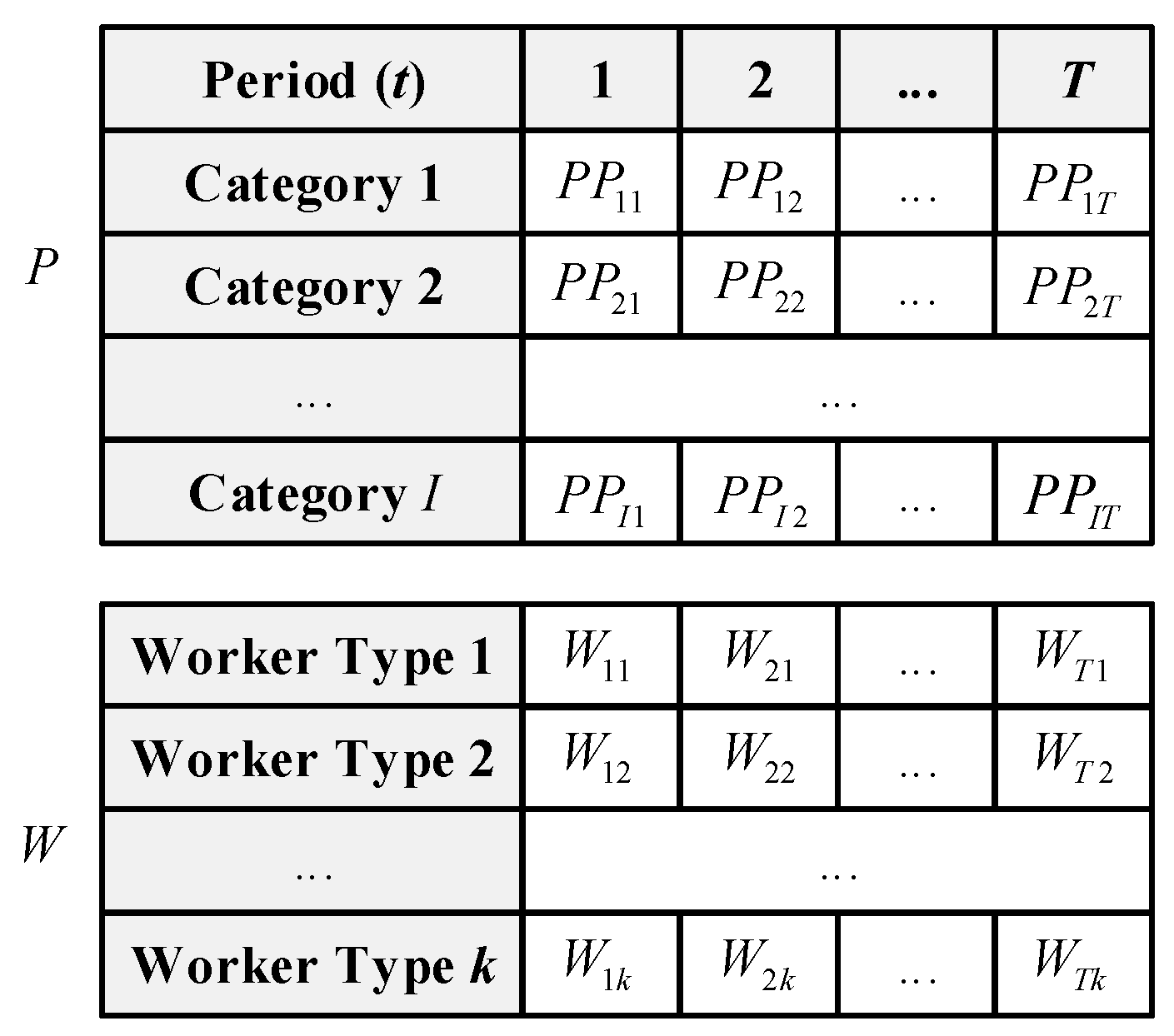
Chromosome Representation

In this study, a chromosome $\mathrm{CH}$ contains two sub-chromosomes, P and W, which represent the production quantity of a product and the number of workers, respectively. The genes in each chromosome are integer. Figure 1 is a simple example of a chromosome with I product categories and T periods.

(2)

Initialization

Analysis of the feasible range of $P{P}_{it}$: For the same product in the same period, production in advance and backordering or loss of sales cannot occur at the same time. If the total amount of demand in the current period and the quantity of backorders in the previous period is greater than the sum of production capacity and inventory at the beginning of the current period, stockout occurs. Therefore, in this case, the product should be produced with the maximum production capacity due to the existence of stockout cost. Otherwise, the minimum $P{P}_{it}$ should meet the sum of the product demand in the planning period and the quantity of backorder in the previous period according to Constraint (20). Thus, the minimum $P{P}_{it}$ in the planning period can be obtained by

$${\mathrm{MinPP}}_{it}=\max \left\{0,\min \left\{P{D}_{it}+{\displaystyle \sum _{t_2=1}^{t-1}{B}_{it-1}(t-t_2)}-C{I}_{it},P{N}_{it}\right\}\right\}$$

(23)

Moreover, the maximum production quantity should not exceed the production capacity and inventory capacity according to Constraints (18) and (19).

$${\mathrm{MaxPP}}_{it}=\min \left\{C{N}_i+P{D}_{it}+{\displaystyle \sum _{t_2=1}^{t-1}{B}_{it-1}(t-t_2)}-C{I}_{it},P{N}_{it}\right\}$$

(24)

Analysis of the feasible range of $W_{tk}$: The minimum and maximum $W_{tk}$ can be obtained according to the production quantity and the labor cost and stability in the workforce ($\lceil \rceil$ indicates rounding up).

$${\mathrm{MinW}}_{tk}=⌈({\displaystyle \sum _{i=1}^{I}P{P}_{it}·P{W}_{ik}})/(WR+WO)⌉$$

(25)

$${\mathrm{MaxW}}_{tk}=\max \left\{W_{tk-1},⌈({\displaystyle \sum _{i=1}^{I}P{P}_{it}·P{W}_{ik}})/WR⌉\right\}$$

(26)

Obviously, the chromosomes satisfy Constraints (18)–(22) in the process of initialization.

Calculation of the stockout quantity: If the total amount of demand in the current period and the quantity of backorders in the previous period is greater than the sum of production capacity and inventory at the beginning of the current period, the products will be out of stock; otherwise, the products will be produced in advance. So, the stockout quantity can be calculated by

$$\max \left\{P{D}_{it}+{\displaystyle \sum _{t^{″}=1}^{t-1}{B}_{it-1}(t-t^{″})-}C{I}_{it}-P{P}_{it},0\right\}$$

(27)

(3)

Genetic Operators

The genetic operators in this paper are almost the same as that of the genetic algorithm in [20], mainly including the partheno crossover operator (only utilizable for sub-chromosome $P$), arithmetic crossover operator, production mutation operator, mutation operator for the number of workers, and repairing infeasible gene operators, which will not be introduced in detail here.

The GA has the characteristics of random multi-point search and implicit parallelism, while a simple genetic algorithm is prone to being premature and has slow convergence. As shown in Figure 2, the same experiment is calculated 10 times using the designed GA, and it can be seen that sometimes the algorithm will fall into the local optimal solution.

3.2. Local Search Algorithm

This LS algorithm searches the neighborhood from a solution of production quantity under the condition that the number of workers remains unchanged to improve $Z_1$. The problem of optimization of production quantity is a special case of the MCF problem, according to [20]. Thus, the LS algorithm for production quantity can be designed based on augmenting cycle.

First, production planning can be dealt with as a network model. Any two unequal periods $t_1,t_2\in [1,T]$ can form a cycle. The maximum adjustment production quantity of i is limited by the minimum value of the production quantity of period $t_1$, the inventory capacity from period $t_1$ to $t_2$, and the production quantity of period $t_2$. The maximum adjustment amount can be determined according to the limit quantity analysis of three aspects for the formed anticlockwise circle and clockwise circle, respectively.

(1)

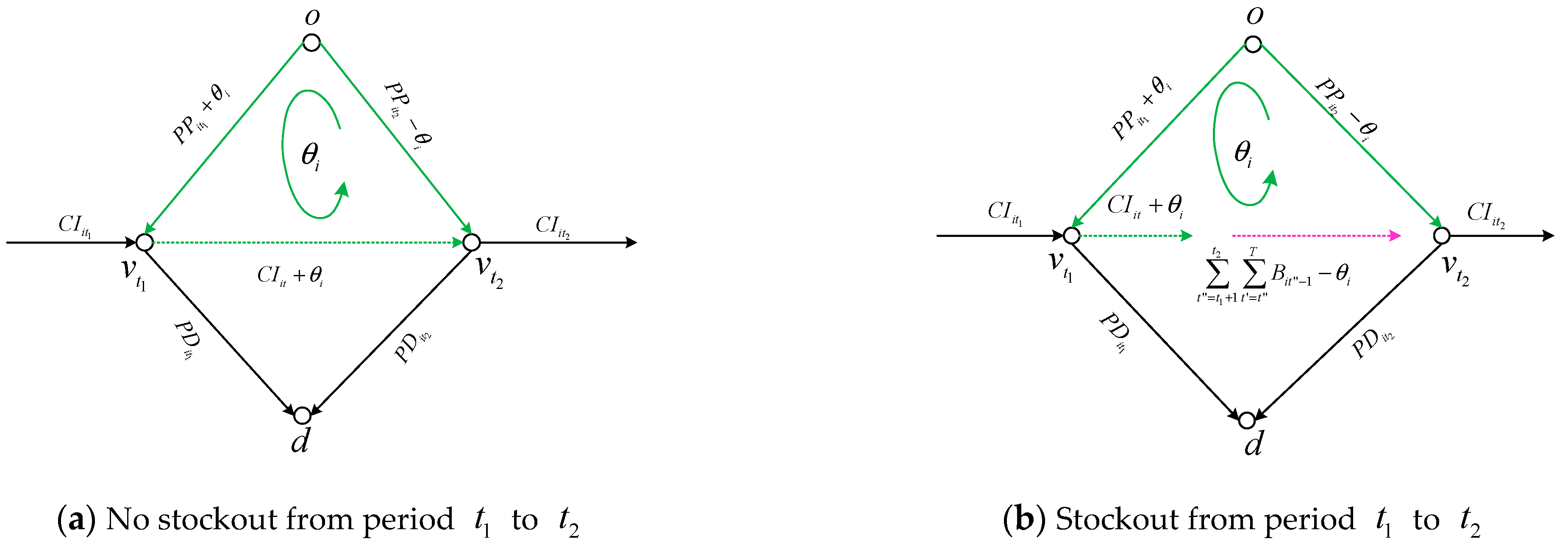
The formed anticlockwise cycle

The production quantity of period $t_1$: The maximum production quantity of the period $t_1$ will limit the increased flow, which can be expressed as ${\mathrm{MaxPP}}_{i{t}_1}-P{P}_{i{t}_1}$.

Inventory remaining capacity: The minimum remaining inventory capacity from period $t_1$ to $t_2$ is $\min \left\{C{N}_i-C{I}_{it}\left|t_1<t\le t_2\right.\right\}$.

The production quantity of period $t_2$: If there is no stockout from period $t_1$ to $t_2$, the adjustment amount of the period $t_2$ limit is $P{P}_{i{t}_2}-{\mathrm{MinPP}}_{i{t}_2}$ (as shown in Figure 3a). Otherwise, the adjustment amount can be increased to the total stockout quantity from period $t_1$ to $t_2$, ${\displaystyle \sum _{t^{″}=t_1+1}^{t_2}{\displaystyle \sum _{t^{\prime }=t^{″}}^T{B}_{i{t}^{″}-1}(t^{\prime }-t^{″}+1)}}$ (as shown in Figure 3b).

The maximum adjustment amount of anticlockwise cycle for product i can be obtained as follows:

$$F{P}_i=\min \left\{{\mathrm{MaxPP}}_{i{t}_1}-P{P}_{i{t}_1},C{N}_i-C{I}_{it},\right.P{P}_{i{t}_2}-{\mathrm{MinPP}}_{i{t}_2}+{\displaystyle \sum _{t^{″}=t_1+1}^{t_2}{\displaystyle \sum _{t^{\prime }=t^{″}}^T{B}_{i{t}^{″}-1}(t^{\prime }-t^{″}+1)}}\left.\left|t_1<t\le t_2\right.\right\}.$$

(28)

(2)

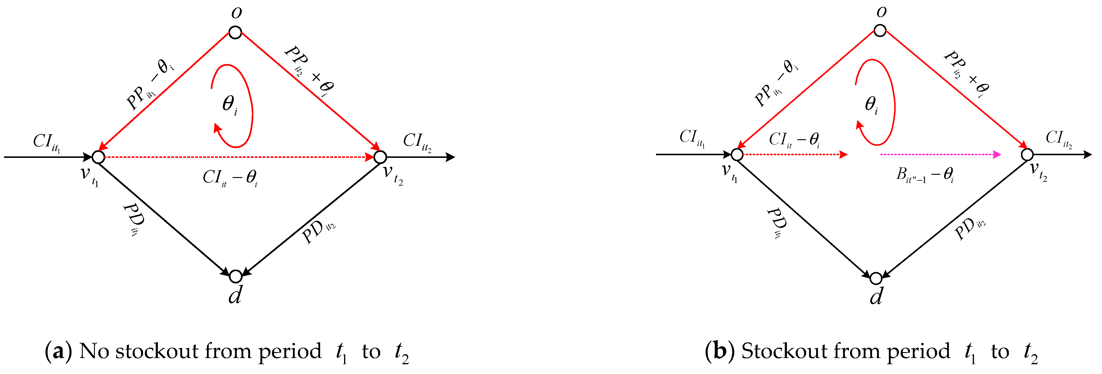
The formed clockwise cycle

The production quantity of period $t_1$: If there is no stockout from period $t_1$ to $t_2$, the adjustment amount of the period $t_1$ limit is $P{P}_{i{t}_1}-{\mathrm{MinPP}}_{i{t}_1}$ (as shown in Figure 4a). Otherwise, the adjustment amount can be increased to the minimum stockout quantity from period $t_1$ to $t_2$: $\min \left\{B_{i{t}^{″}-1}(t^{\prime }-t^{″}+1)\left|t_1\le t^{″}<t_2,t^{″}\le t^{\prime }\le T\right.\right\}$ (as shown in Figure 4b).

Inventory remaining capacity: The minimum remaining inventory capacity from period $t_1$ to $t_2$ is $\min \left\{C{I}_{it}\left|C{I}_{it}>0,t_1<t\le t_2\right.\right\}$.

The production quantity of period $t_2$: The maximum production quantity of the period $t_2$ will limit the increased flow, which can be expressed as ${\mathrm{MaxPP}}_{i{t}_2}-P{P}_{i{t}_2}$.

The maximum adjustment amount of clockwise cycle for product i can be obtained by

$$\begin{array}{c}F{P}_i=\min \left\{{\mathrm{MaxPP}}_{i{t}_2}-P{P}_{i{t}_2},C{I}_{it},B_{i{t}^{″}-1}(t^{\prime }-t^{″}+1),\right.\hfill \\ \hfill \left.\hspace{1em}\hspace{1em}P{P}_{i{t}_1}-{\mathrm{MinPP}}_{i{t}_1}+\min \{B_{i{t}^{″}-1}(t^{\prime }-t^{″}+1)\}|C{I}_{it}>0,t_1<t\le t_2\right\}.\end{array}$$

(29)

LS algorithm can significantly improve the quality of solution, especially in large-scale experiments, as shown in Figure 5. However, the running time will be greatly increased for each experiment.

3.3. Double-Layered Multi-Objective Particle Swarm Optimization Algorithm

In the PSO model, each particle needs to continuously update the velocity and the position according to the Pbest (the best position of a particle) and the Gbest (the best position for all particles). For the single-objective problem, these two solutions are easy to choose, but for the multi-objective problem, it is difficult to choose the local optimal guide Pbest and the global optimal guide Gbest. How to choose the Pbest and the Gbest to guide the moving of each particle in the search space is a critical issue, and it is very important for the premature convergence of the PSO algorithm and the diversity of solutions [27].

(1)

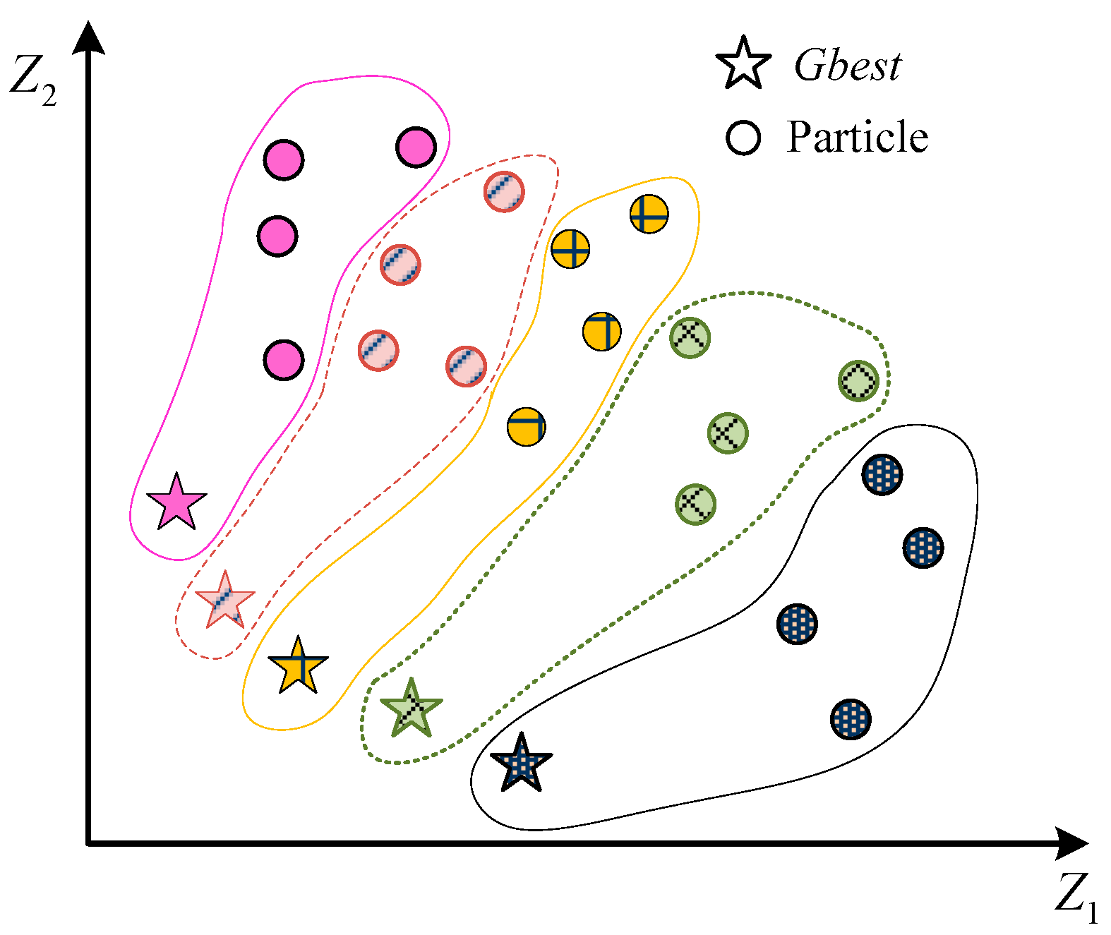
Generation and Update of the Global Optimal Guide

Choosing an appropriate global optimal solution, Gbest, to guide particles will greatly improve the quality of Pareto solutions and maintain the diversity of nondominated solutions. Firstly, this paper establishes an external archive, which mainly records the nondominated solutions found so far. At each iteration, the external archive is updated to ensure that the external archive is only nondominated solutions.

Selection mechanism of Gbest: The following selection mechanism of Gbest is established based on the external archive: If the number of nondominated solutions in the external archive is less than or equal to the population size of the PSO algorithm, popsize, all the solutions in the external archive are selected as the global optimal guides Gbest. Otherwise, the crowding distance-based selection algorithm is used to select popsize solutions from the external archive as the global optimal guides Gbest.

Gbest assignment mechanism for each particle: Let NDnum be the number of solutions in Gbest, and the mechanism for assigning a global optimal guide to each particle is as follows:

Step 1. Calculate the distance between individual particles and the solutions in Gbest.

Step 2. Assign a guide to each particle. If NDnum=popsize, select a guide with the smallest distance for each particle as the individual global optimal guide (the global optimal guides for individual particles cannot be repeated). Otherwise, each global optimal guide is assigned to popsize/NDnum particles with the smallest distance as their global optimal guides.

Figure 6 shows the Gbest assignment mechanism for each particle of the bi-objective optimal problem.

(2)

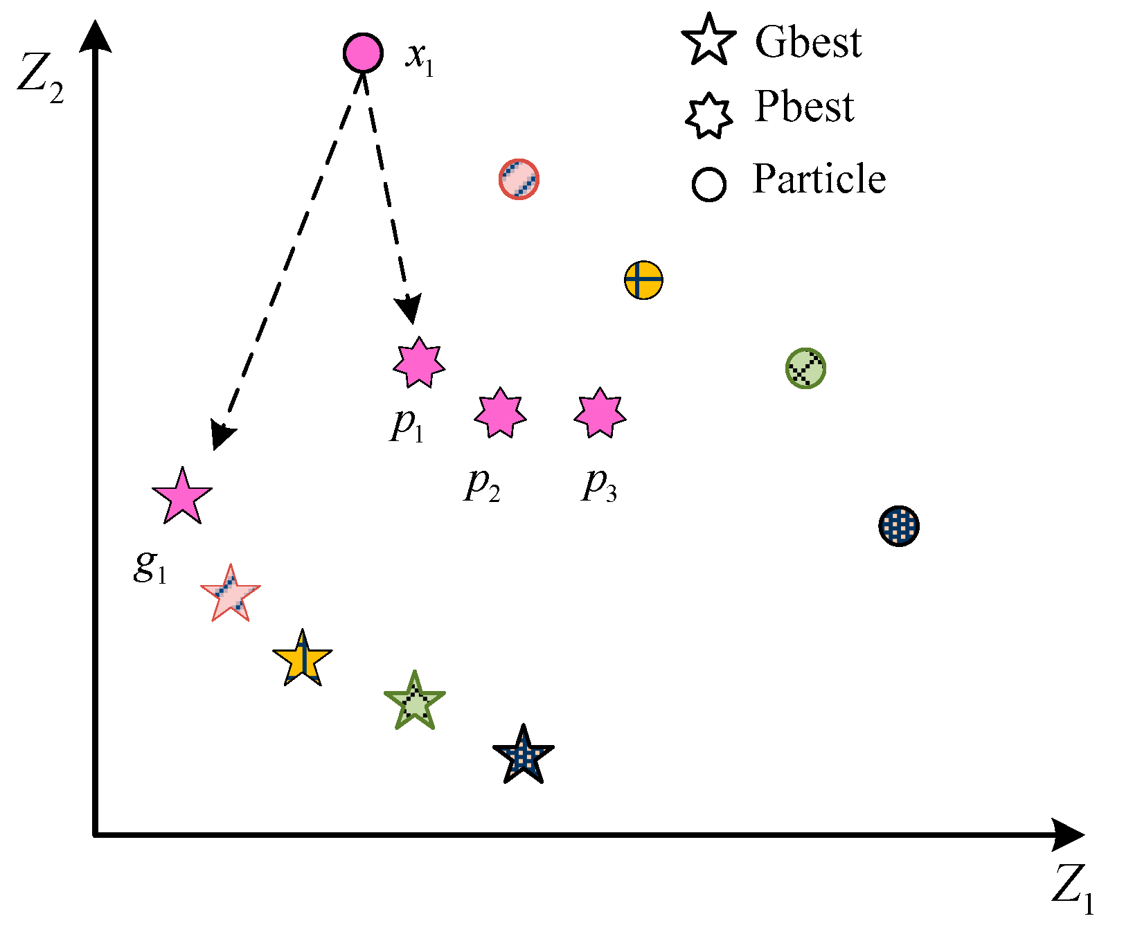
Selection Mechanism of the Local Optimal Guide Pbest

During the evolution process of the PSO algorithm, the local optimal guide Pbest is selected for each particle according to the following method: Calculate the distance between each solution in the Pbest set and the global optimal guide corresponding to the individual in Gbest, and select the individual optimal location with the smallest distance as the local optimal guide. Figure 7 visualizes this process. $g_1$ is the global optimal guide assigned to an individual particle $x_1$. $p_1,p_2,p_3$ are the solutions in the Pbest for $x_1$. When selecting the local optimal guide for $x_1$, $p_1$ is selected because its position is closest to $g_1$.

(3)

Updating Rules of Particle Velocity and Position

In the standard form of PSO, the velocity vector for particle k is updated according to three other vectors that are the local optimal guide of the kth particle (Pbest), the current global optimal guide (Gbest), and the current position of the particle [28]. In every iteration, each particle updates its velocity and position according to the assigned global optimal guide and local optimal guide according to the following rules:

$$v_k^1(g+1)=\chi \left[{\omega }_k{v}_k^1(g)+c_1{r}_1(p{b}_k^1(g)-x_k^1(g))+c_2{r}_2(g{b}_k^1(g)-x_k^1(g))\right]$$

(30)

$$v_k^2(g+1)=\chi \left[{\omega }_k{v}_k^2(g)+c_1{r}_1(p{b}_k^2(g)-x_k^2(g))+c_2{r}_2(g{b}_k^2(g)-x_k^2(g))\right]$$

(31)

$$x_k^1(g+1)=x_k^1(g)+⌈v_k^1(g+1)⌉$$

(32)

$$x_k^2(g+1)=x_k^2(g)+⌈v_k^2(g+1)⌉$$

(33)

where k is a particle, $\chi$ is the constriction factor, and ${\omega }_k$ is the inertia weight. $c_1$, $c_2$ are respectively learning factors. $r_1$, $r_2$ are two random parameters within [0, 1]. $g$ is the number of iterations, $v_k^1(g)$ and $v_k^2(g)$ represent the velocity of particle k in the PP layer and W layer of iteration g, respectively. $p{b}_k^1(g)$, $p{b}_k^2(g)$, $g{b}_k^1(g)$ and $g{b}_k^2(g)$ represent the local optimal guide and global optimal guide of particle k in the PP layer and W layer of iteration g, respectively. $x_k^1(g)$ and $x_k^2(g)$ are the position of particle k.

Generally, a large inertial weight facilitates the global search, while a small inertial weight facilitates the local search. Therefore, a linearly decreasing inertial weight is adopted to adjust ${\omega }_k$.

$${\omega }_k(g)={\omega }_{\max }-\frac{g({\omega }_{\max }-{\omega }_{\min })}{G}$$

(34)

where G is the maximum iteration number, ${\omega }_{\max }$ and ${\omega }_{\min }$ are the predefined maximum and minimum inertia weight, respectively.

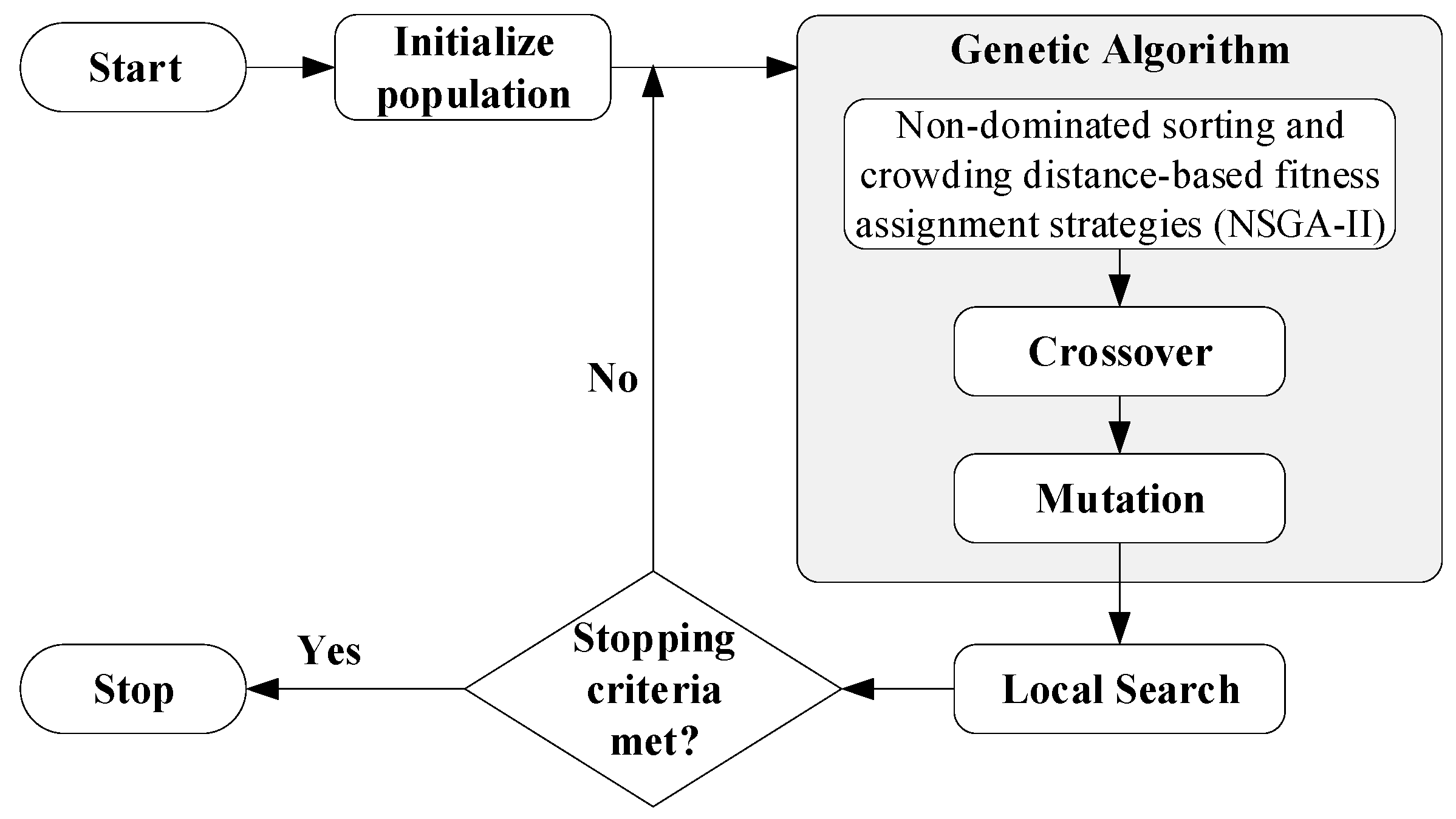
3.4. Hybrid Strategies

In order to improve the efficiency of solving large-scale multi-objective APP problems, based on the characteristics of GA, LS, and PSO, this section designs three different hybrid strategies.

(1)

Hybrid Strategy of LS-GA

The idea of LS-GA hybrid strategy is to use the local search ability of LS to improve the efficiency of the algorithm. The method is to add an LS search algorithm in the evolution process of each offspring. The flow chart of the LS-GA Strategy is shown in Figure 8.

(2)

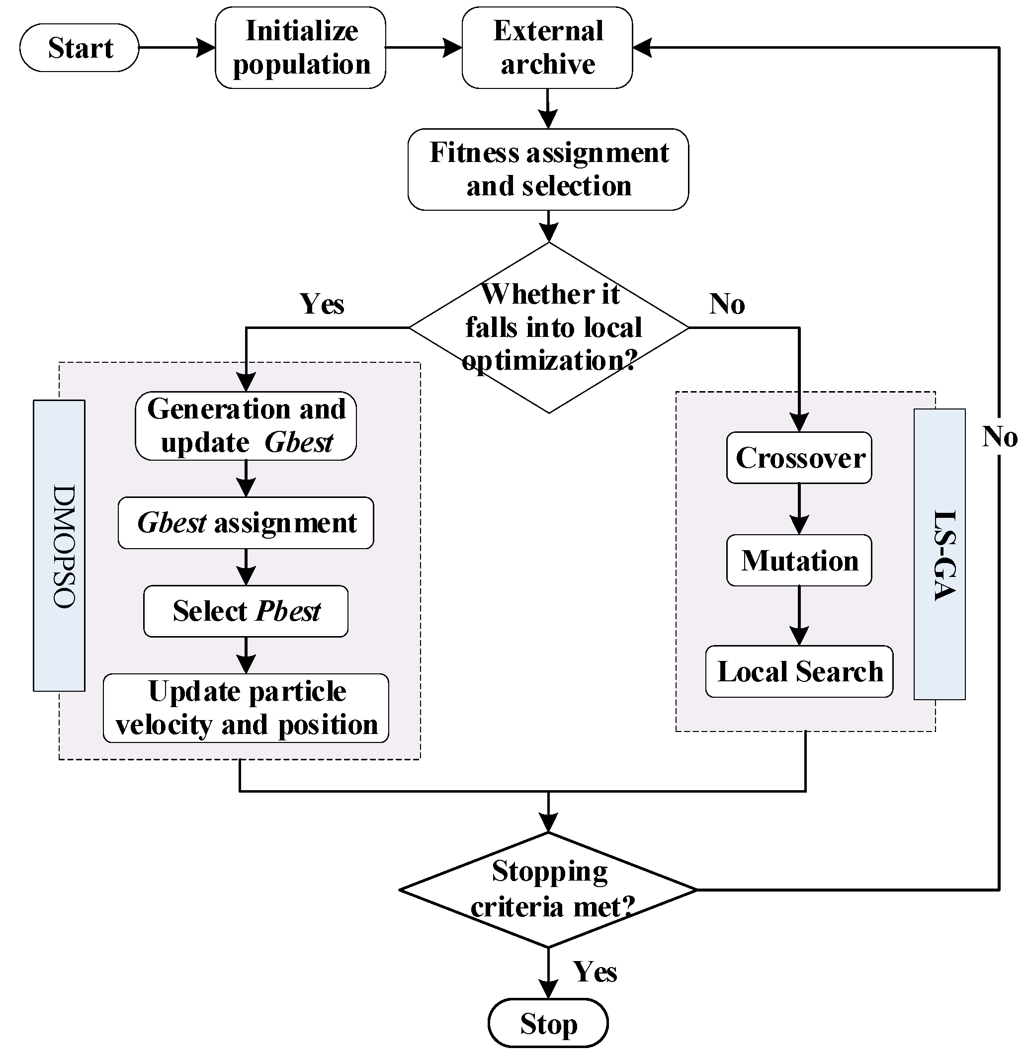
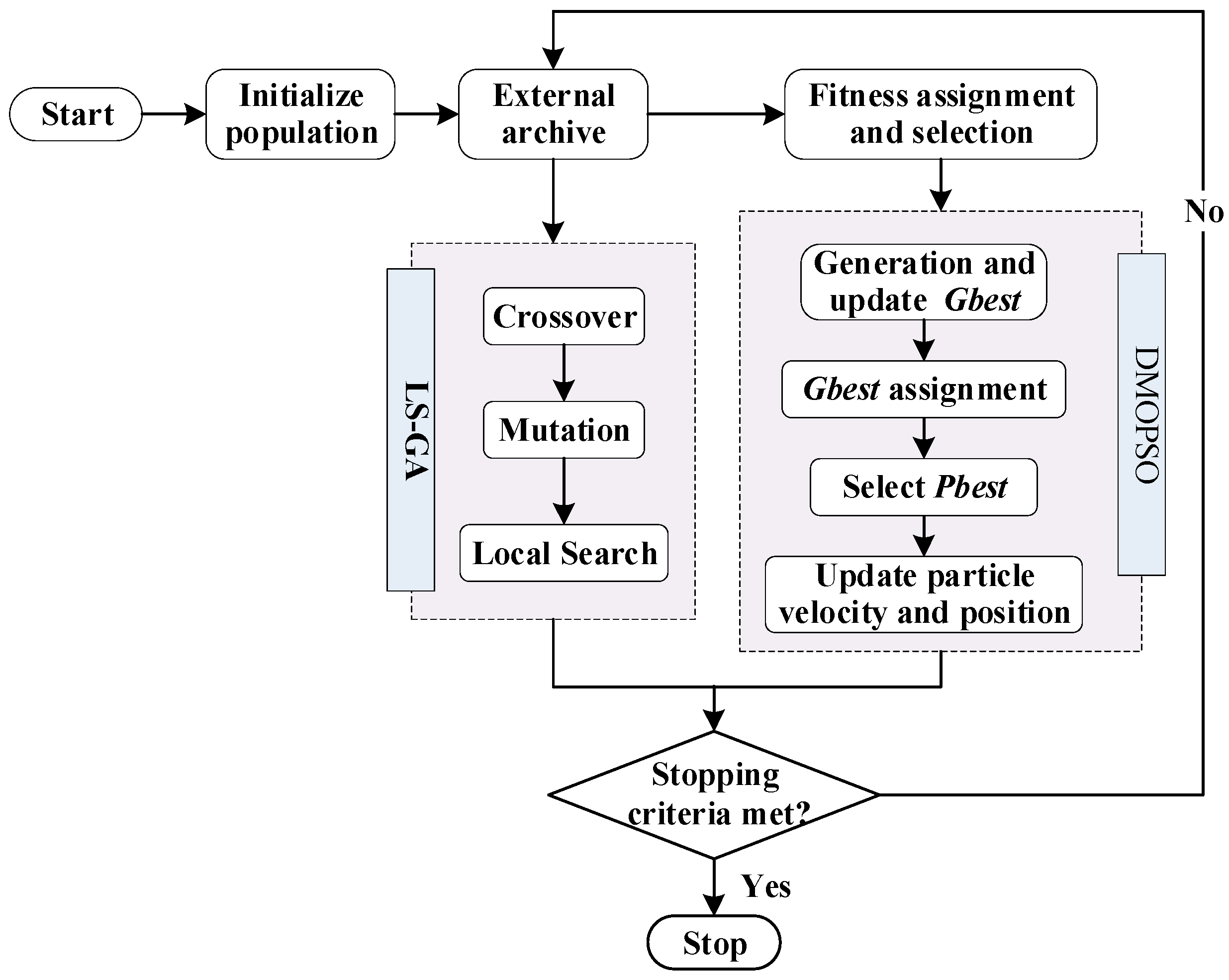
Hybrid Strategy of HGA-PSO1

The hybrid genetic algorithm-particle swarm optimization based on stages (HGA-PSO1) combines the PSO algorithm and LS-GA algorithm, considering the characteristics of the PSO algorithm, which has fast convergence speed but is prone to premature convergence, and the LS-GA algorithm has strong local search ability.

One of the methods of this strategy is: Firstly, the DMOPSO algorithm is used for global search. When it falls into the local optimal solution (by setting a certain evolutionary algebra), then the LS-GA algorithm is used for local search based on the global optimal solution. The flow chart of the hybrid strategy for HGA-PSO1 is shown in Figure 9.

(3)

Hybrid Strategy of HGA-PSO2

The other method of hybrid strategy based on LS-GA and PSO is: The population is divided into two subpopulations for LS-GA and PSO, and nondominated sorting and crowding distance-based fitness assignment strategies of the NSGA-II algorithm are used to implement the competitive selection. LS-GA selects the initial population from the external archive by selection operation to optimize the solution in the external archive, and PSO selects individual particles from the overall parent population for global search. The flow chart of the hybrid strategy of HGA-PSO2 is shown in Figure 10.

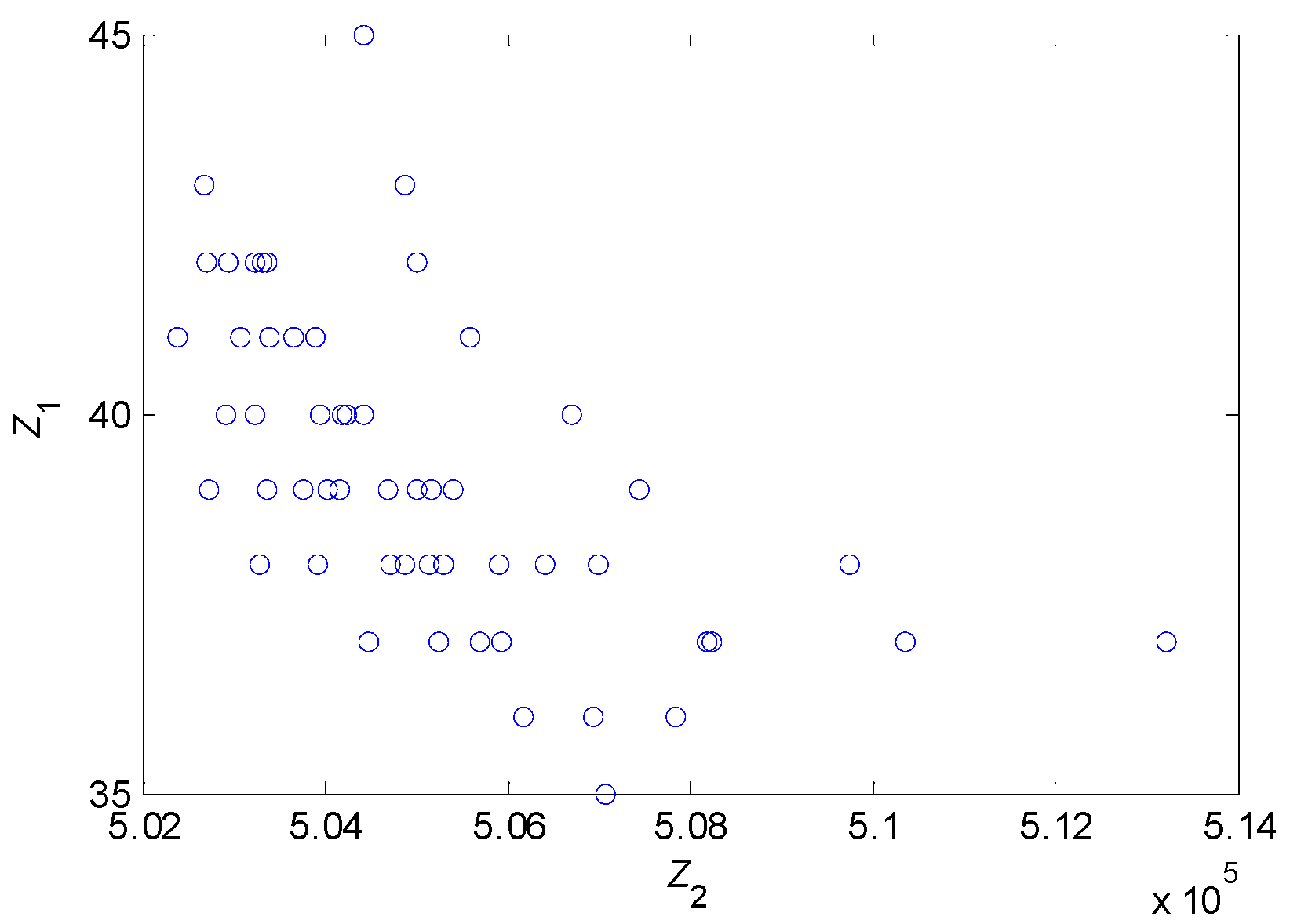
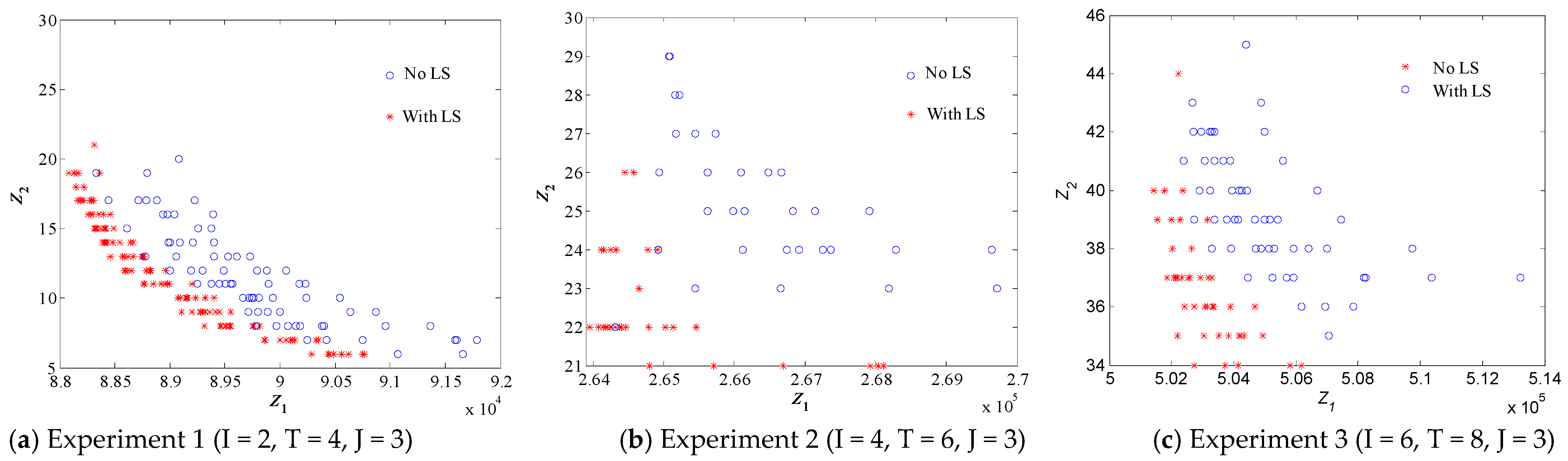
4. Numerical Experiments

For comparing the performance of LS-GA, HGA-PSO1, and HGA-PSO2, all algorithms solve nine test experiments 10 times, and the performance measures defined in [20], the average objectives value ($\mathrm{avg}(·)$), the runtime of the algorithm (Runtime (S)), the number of nondominated sets ($M_1$), set coverage measure ($M_2$), and mean ideal distance (MID), are used to analyze the performance of algorithms.

The main parameters of the test experiments are listed in

Table 6. Parameters setting.

Experiments				Parameters of Labors
No.	I	T	J	Parameter	Value
1	2	4	3	$WHC$ (Yuan/p)	100
2	2	6	3	$WR$ (h)	50
3	2	8	3	$WO$ (h)	10
4	4	4	3	$W{I}_k$ (Yuan)	800
5	4	6	3	$WR{C}_k$ (Yuan/h)	5
6	4	8	3	$WO{C}_k$ (Yuan/h)	10
7	6	4	3	$W_{1k}$ (p)	10
8	6	6	3
9	6	8	3

(k = 1), and other parameters are described in

Table A1. Production capacity of experiments.

Experiment No.	i	t
		1	2	3	4	5	6	7	8
1	1	50	90	190	260	--	--	--	--
	2	40	40	50	100	--	--	--	--
2	1	50	80	180	250	200	200	--	--
	2	50	50	50	100	100	90	--	--
3	1	50	80	175	260	210	200	150	150
	2	50	50	50	100	80	80	80	80
4	1	50	100	150	280	--	--	--	--
	2	50	80	50	80	--	--	--	--
	3	50	50	70	70	--	--	--	--
	4	100	110	100	110	--	--	--	--
5	1	50	110	150	250	250	200	--	--
	2	50	80	80	80	80	80	--	--
	3	60	60	60	70	70	70	--	--
	4	100	110	100	100	100	120	--	--
6	1	50	100	150	260	250	200	150	150
	2	50	80	80	100	80	80	80	80
	3	60	60	60	70	80	80	80	70
	4	100	100	100	120	120	120	100	100
7	1	60	100	200	200	--	--	--	--
	2	60	70	70	80	--	--	--	--
	3	60	60	70	70	--	--	--	--
	4	120	110	100	120	--	--	--	--
	5	70	70	70	70	--	--	--	--
	6	90	90	100	90	--	--	--	--
8	1	70	150	200	250	220	200	--	--
	2	80	80	80	80	80	80	--	--
	3	70	70	70	80	80	80	--	--
	4	80	100	100	150	100	150	--	--
	5	80	80	80	80	80	80	--	--
	6	90	100	100	90	100	100	--	--
9	1	60	70	150	250	220	200	200	200
	2	80	80	100	100	100	100	100	80
	3	70	70	70	80	80	80	80	80
	4	90	150	100	150	150	150	100	100
	5	90	85	80	80	90	100	95	90
	6	100	95	105	100	100	95	105	100

,

Table A2. Parameters of production and raw materials.

Parameters	i, j	t
		1	2	3	4	5	6	7	8
$P{D}_{it}$ (unit)	1	85.0	125.0	175.0	250.0	200.0	180.0	150.0	120.0
	2	30.0	45.0	50.0	80.0	70.0	65.0	55.0	60.0
	3	50.0	55.0	60.0	70.0	55.0	75.0	60.0	65.0
	4	100.0	120.0	90.0	110.0	100.0	120.0	90.0	85.0
	5	50.0	70.0	65.0	70.0	50.0	80.0	85.0	90.0
	6	80.0	85.0	95.0	75.0	80.0	85.0	90.0	95.0
$P{C}_i$ (Yuan/unit)	1	28.8	28.8	28.8	28.8	28.8	28.8	28.8	28.8
	2	23.0	23.0	23.0	23.0	23.0	23.0	23.0	23.0
	3	20.0	20.0	20.0	20.0	20.0	20.0	20.0	20.0
	4	30.0	30.0	30.0	30.0	30.0	30.0	30.0	30.0
	5	20.0	20.0	20.0	20.0	20.0	20.0	20.0	20.0
	6	22.0	22.0	22.0	22.0	22.0	22.0	22.0	22.0
$P{W}_{ik}$ (h/unit)	1	3.8	3.8	3.8	3.8	3.8	3.8	3.8	3.8
	2	5.7	5.7	5.7	5.7	5.7	5.7	5.7	5.7
	3	6.0	6.0	6.0	6.0	6.0	6.0	6.0	6.0
	4	4.0	4.0	4.0	4.0	4.0	4.0	4.0	4.0
	5	5	5	5	5	5	5	5	5
	6	6.5	6.5	6.5	6.5	6.5	6.5	6.5	6.5
$P{N}_{it}$ (unit)	1	100.0	170.0	200.0	255.0	220.0	210.0	200.0	200.0
	2	80.0	80.0	150.0	110.0	100.0	100.0	100.0	80.0
	3	70.0	75.0	75.0	75.0	80.0	80.0	95.0	90.0
	4	150.0	150.0	160.0	150.0	150.0	140.0	150.0	140.0
	5	90.0	85.0	80.0	80.0	90.0	100.0	95.0	90.0
	6	100.0	95.0	105.0	100.0	100.0	95.0	105.0	100.0
$R{C}_{jt}$ (Yuan/unit)	1	2.0	2.0	3.0	1.0	2.0	2.0	2.0	3.0
	2	3.0	2.0	3.0	3.0	2.0	2.0	3.0	2.0
	3	3.0	3.5	3.0	2.8	3.0	4.0	3.0	3.5

and

Table A3. Parameters of inventory and raw materials.

Parameters		i
		1	2	3	4	5	6
$C{I}_{i1}$ (unit)		65.0	29.0	10.0	20.0	15.0	25.0
$C{K}_i$ (Yuan)		15.0	2.0	3.0	3.0	4.0	3.0
$C{N}_i$ (unit)		100.0	50.0	70.0	100.0	55.0	60.0
$R_{ij}$ (unit)	1	0.8	0.3	0.2	0.5	0.4	0.1
	2	0.5	0.5	0.3	0.2	0.2	0.4
	3	0.0	0.4	0.3	0.6	0.1	0.2

of Appendix A. Several parameters, such as the population sizes, the maximum number of generations, the probability of the crossover, and the mutation operator, may influence the performance of an algorithm. In this research, all the parameters of the GA and PSO algorithms are relatively efficient values obtained through many tests, which are shown in

Table 7. Parameters of the GA and PSO.

Parameter Setting of GA		Parameter Setting of PSO
Parameter	Value	Parameter	Value
Population sizes $popsize$	Experiments 1~3: 30, each sub-population of HGA-PSO2: 15 Experiments 4~6: 40, each sub-population of HGA-PSO2: 20 Experiments 7~9: 50, each sub-population of HGA-PSO2: 25	Constriction factor $$	0.73
Maximum number of generations G	Experiments 1~3: 1000, Set algebra of HGA-PSO1: 500 Experiments 4~6: 1200, Set algebra of HGA-PSO1: 600 Experiments 7~9: 1500, Set algebra of HGA-PSO1: 750	Predefined maximum value of inertia weight ${\omega }_{\max }$	0.8
Probability of partheno crossover operator: $P_{c1}$	Iteration number < 600: 0.2, otherwise, 0.3	Predefined minimum value of inertia weight ${\omega }_{\min }$	0.4
Probability of arithmetic crossover $P_{c2}$	Iteration number < 600: 0.1, otherwise, 0.2	Learning factors $c_1$	2.0
Probability of production mutation $P_{m1}$	Iteration number < 600: 0.4, otherwise, 0.6	Learning factors $c_2$	2.1
Probability of mutation for the number of workers $P_{m2}$	Iteration number < 600: 0.5, otherwise, 0.7

. Moreover, the backordering intensity coefficient $k_0=0.25$, the waiting time resistance $k_1=0.3$, the fixed cost part of product i $f_i=0.05P{C}_i$, the cost rate $a_i=0.5f_i$, and the cost increasing rate $b_i=0.05f_i$, respectively. The rates of customer loss threshold and backorder cost per unit quantity are shown in Figure 11 and Figure 12, respectively.

The experiments are performed on DELL Vostro 3800-R1846 (Intel Core i3 4130 (3.4 GHz 8 GB memory)) 10 times. The results of performance measures are reported in

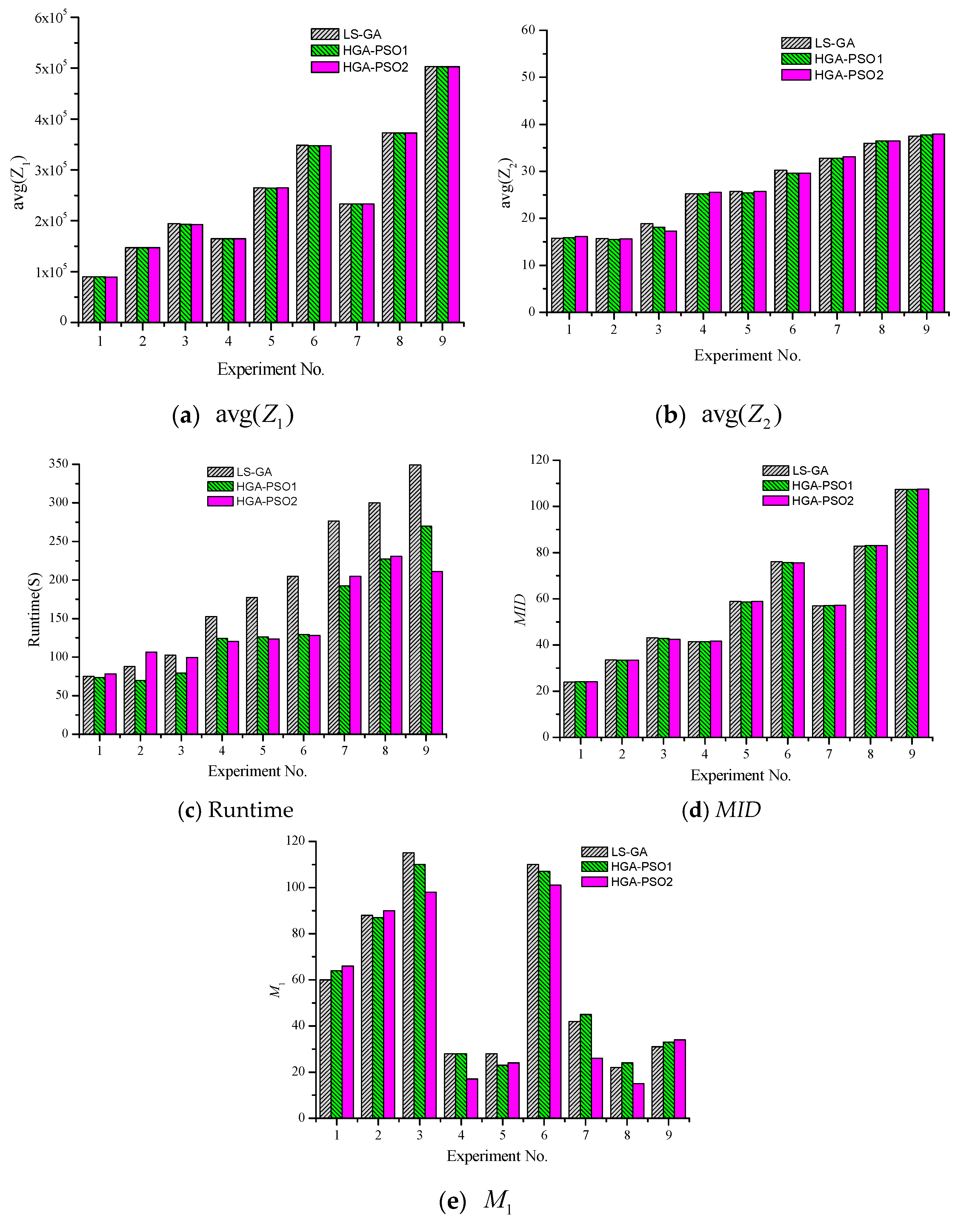
Table 8. The results of performance measures.

Performance Measure	Hybrid Strategy	Experiment No.
		1	2	3	4	5	6	7	8	9
$\mathrm{avg}(Z_1)$/(104)	LS-GA	8.96	14.71	19.42	16.47	26.44	34.84	23.32	37.28	50.29
	HGA-PSO1	8.96	14.71	19.31	16.47	26.44	34.76	23.32	37.26	50.27
	HGA-PSO2	8.95	14.71	19.27	16.46	26.45	34.75	23.31	37.26	50.29
$\mathrm{avg}(Z_2)$	LS-GA	15.78	15.66	18.83	25.21	25.75	30.23	32.76	36.00	37.45
	HGA-PSO1	15.83	15.52	18.07	25.21	25.39	29.58	32.80	36.50	37.70
	HGA-PSO2	16.08	15.61	17.26	25.53	25.75	29.63	33.08	36.47	37.97
Runtime/(S)	LS-GA	75.28	87.86	102.54	152.64	177.57	204.66	276.56	300.18	348.90
	HGA-PSO1	73.57	69.64	79.40	124.25	126.31	129.35	192.50	227.47	341.08
	HGA-PSO2	78.22	106.39	99.46	120.52	123.45	127.95	204.67	230.62	210.89
$M_1$	LS-GA	60	88	115	28	28	110	42	22	31
	HGA-PSO1	64	87	110	28	23	107	45	24	33
	HGA-PSO2	66	90	98	17	24	101	26	15	34
$M_2$	LS-GA, HGA-PSO1	−0.03	−0.08	−0.87	0.21	−0.20	−0.46	0.18	0.09	−0.28
	LS-GA, HGA-PSO2	−0.08	−0.09	−0.97	0.58	0.18	−0.35	0.35	0.06	0.24
	HGA-PSO1, LS-GA	0.03	0.08	0.87	−0.21	0.20	0.46	−0.18	−0.09	0.28
	HGA-PSO1, HGA-PSO2	−0.05	−0.08	0.14	0.23	0.39	0.07	0.05	−0.08	0.54
	HGA-PSO2, LS-GA	0.08	0.09	0.97	−0.58	−0.18	0.35	−0.35	−0.06	−0.24
	HGA-PSO2, HGA-PSO1	0.05	0.08	−0.14	−0.23	−0.39	−0.07	−0.05	0.08	−0.54
MID	LS-GA	23.97	33.43	43.17	41.50	58.83	76.02	57.00	82.81	107.34
	HGA-PSO1	23.99	33.36	42.82	41.49	58.67	75.64	57.03	82.99	107.38
	HGA-PSO2	24.14	33.40	42.38	41.66	58.83	75.62	57.17	82.97	107.51

and Figure 13, respectively.

From the comparison results of performance measures $\mathrm{avg}(Z_1)$, $\mathrm{avg}(Z_2)$, $M_1$ and MID, there is little difference in the performance of LS-GA, HGA-PSO1, and HGA-PSO2 algorithms. From the algorithm running time, HGA-PSO1 and HGA-PSO2 algorithms have less average runtime than the LS-GA strategy, and the larger the problem scale, the greater the difference in running time. Moreover, the $M_2$ in Table 8 shows that the overall performances of HGA-PSO1 and HGA-PSO2 are slightly better than that of LS-GA, and there is no significant difference between HGA-PSO1 and HGA-PSO2 strategies. The obtained solutions of three hybrid strategies are compared in Figure 14. The results show that there is no significant difference in the number of nondominated sets obtained by the three hybrid strategies.

5. Discussion and Conclusions

The increasingly fierce market competition makes enterprises face the changing market environment. The diversity of products and fierce competition make the stability of the manufacturing industry and supply chain more important than ever. In order to adapt to the rapidly changing market demand, more and more manufacturing enterprises choose the coexistence of order-oriented and inventory-oriented multi-variety and small batch production. The change in demand level will lead to a change in enterprise employment, and the change in employees will lead to a change in workers’ labor efficiency and labor cost. Therefore, decision makers pay great attention to the impact of labor changes, and the stability of workers has become more important than ever.

Due to the decline of actual production capacity or the shortage of production materials, production enterprises may be backordered. Generally, the method of penalty cost is adopted to deal with the BC, and the BC per unit time is fixed, and most of them do not consider the difference in the time to replenishment. In fact, the longer the replenishment time and the greater the backorder quantity, the greater the possibility of a loss of sales and the worse the customer satisfaction. Therefore, the impact of early and late delivery is analyzed, and the threshold for customer loss and the BC per unit time is defined by considering the dual effects of replenishment time and backorder quantity.

Then, the maximum tolerant backorder quantity of customers in different delay periods is calculated according to the demand for products. In considering the waiting time and the quantity of backorder, the delayed delivery cost varying with the waiting time is designed, and the cost of delayed delivery and loss of sales is determined. Considering the production cost, raw material cost, inventory cost, staff cost, stockout, and lost sales cost, an early/delayed multi-objective optimization model is developed for an APP problem of multi-product.

Moreover, three algorithms, GA, LS, and DMOPSO, and three different hybrid strategies, are designed to solve the model, and the experiments are performed on some testing examples. The computational results indicated that the determination of the feasible range of product output and the number of workers in the workforce can reduce the search scope and improve the efficiency of the algorithm. HGA-PSO1 and HGA-PSO2 strategies have less average runtime than the LS-GA strategy, and the larger the problem scale, the greater the difference in running time. In the future, the uncertainty of product demand and production capacity will be taken into account to design the related APP model and algorithm.

References

1. Cheraghalikhani, A.; Khoshalhan, F.; Mokhtari, H. Aggregate production planning: A literature review and future research directions. Int. J. Ind. Eng. Comput. 2019, 10, 309–330. [Google Scholar] [CrossRef]
2. Hu, W.T.; Kim, S.L.; Banerjee, A. An inventory model with partial backordering and unit backorder cost linearly increasing with the waiting time. Eur. J. Oper. Res. 2009, 197, 581–587. [Google Scholar] [CrossRef]
3. Wang, R.C.; Liang, T.F. Aggregate production planning with multiple fuzzy goals. Int. J. Adv. Manuf. Technol. 2005, 25, 589–597. [Google Scholar] [CrossRef]
4. Ning, Y.F.; Tang, W.S.; Zhao, R.Q. Multi-product aggregate production planning in fuzzy random environments. World J. Model. Simul. 2006, 22, 312–321. [Google Scholar]
5. Mahdavi, I.; Aalaei, A.; Paydar, M.M.; Solimanpur, M. Designing a mathematical model for dynamic cellular manufacturing systems considering production planning and worker assignment. Comput. Math. Appl. 2010, 60, 1014–1025. [Google Scholar] [CrossRef] [Green Version]
6. Chakrabortty, R.K.; Hasin, M.A.A. Solving an aggregate production planning problem by using multi-objective genetic algorithm (MOGA) approach. Int. J. Ind. Eng. Comput. 2013, 4, 1–12. [Google Scholar] [CrossRef]
7. Sadeghi, M.; Razavi Hajiagha, S.H.; Hashemi, S.S. A fuzzy grey goal programming approach for aggregate production planning. Int. J. Adv. Manuf. Technol. 2013, 64, 1715–1727. [Google Scholar] [CrossRef]
8. Saidi-Mehrab Ad, M.; Paydar, M.M.; Aalaei, A. Production planning and worker training in dynamic manufacturing systems. J. Manuf. Syst. 2013, 32, 308–314. [Google Scholar] [CrossRef]
9. Basis, H.; Lu, S.; Su, H.Y.; Wang, Y.; Xie, L.; Zhang, Q.L. Multi-product multi-stage production planning with lead time on a rolling. IFAC PapersOnLine 2015, 48, 1162–1167. [Google Scholar] [CrossRef]
10. Modarres, M.; Izadpanahi, E. Aggregate production planning by focusing on energy saving: A robust optimization approach. J. Clean. Prod. 2016, 133, 1074–1085. [Google Scholar] [CrossRef]
11. Hossain, M.M.; Nahar, K.; Reza, S.; Shaifullah, K.M. Multi-period, multi-product, aggregate production planning under demand uncertainty by considering wastage cost and incentives. World Rev. Bus. Res. 2016, 6, 170–185. [Google Scholar]
12. Sakhaii, M.; Tavakkoli-Moghaddam, R.; Bagheri, M.; Vatani, B. A robust optimization approach for an integrated dynamic cellular manufacturing system and production planning with unreliable machines. Appl. Math. Model. 2016, 40, 169–191. [Google Scholar] [CrossRef]
13. Mehdizadeh, E.; Niaki, S.T.A.; Hemati, M. A bi-objective aggregate production planning problem with learning effect and machine deterioration: Modeling and solution. Comput. Oper. Res. 2018, 91, 21–36. [Google Scholar] [CrossRef]
14. Jamalnia, A.; Yang, J.B.; Xu, D.L.; Feili, A.; Jamali, G. Evaluating the performance of aggregate production planning strategies under uncertainty in soft drink industry. J. Manuf. Syst. 2019, 50, 146–162. [Google Scholar] [CrossRef] [Green Version]
15. Xue, G.S.; Offodile, O.F. Integrated optimization of dynamic cell formation and hierarchical production planning problems. Comput. Ind. Eng. 2020, 139, 106155. [Google Scholar] [CrossRef]
16. Jang, J.; Chung, B.D. Aggregate production planning considering implementation error: A robust optimization approach using bi-level particle swarm optimization. Comput. Ind. Eng. 2020, 142, 106367. [Google Scholar] [CrossRef]
17. Florian, M.; Lenstra, J.K.; Rinnooy Kan, A.H.G. Deterministic production planning: Algorithms and complexity. Manag. Sci. 1980, 26, 669–679. [Google Scholar] [CrossRef]
18. Chen, W.H.; Thizy, J.M. Analysis of relaxations for the multi-item capacitated lot-sizing problem. Ann. Oper. Res. 1990, 26, 29–72. [Google Scholar] [CrossRef]
19. Ramezanian, R.; Rahmani, D.; Barzinpour, F. An aggregate production planning model for two phase production systems: Solving with genetic algorithm and tabu search. Expert Syst. Appl. 2012, 39, 1256–1263. [Google Scholar] [CrossRef]
20. Liu, L.F.; Yang, X.F. Multi-objective aggregate production planning for multiple products: A local search-based genetic algorithm optimization approach. Int. J. Comput. Intell. Syst. 2021, 14, 156. [Google Scholar] [CrossRef]
21. Wang, S.C.; Yeh, M.F. A modified particle swarm optimization for aggregate production planning. Expert Syst. Appl. 2014, 41, 3069–3077. [Google Scholar] [CrossRef]
22. Chakrabortty, R.K.; Hasin, M.A.A.; Sarker, R.A.; Essam, D.L. A possibilistic environment based particle swarm optimization for aggregate production planning. Comput. Ind. Eng. 2015, 88, 366–377. [Google Scholar] [CrossRef]
23. Ramachandran, G.M.; Neelakrishnan, S. An approach to improving customer on-time delivery against the original promise date. S. Afr. J. Ind. Eng. 2017, 28, 109–119. [Google Scholar] [CrossRef] [Green Version]
24. Liu, X.; Tu, Y. Production planning with limited inventory capacity and allowed stockout. Int. J. Prod. Econ. 2008, 111, 180–191. [Google Scholar] [CrossRef]
25. Dye, C.Y.; Hsieh, T.P.; Ouyang, L.Y. Determining optimal selling price and lot size with a varying rate of deterioration and exponential partial backlogging. Eur. J. Oper. Res. 2007, 181, 668–678. [Google Scholar] [CrossRef]
26. Yu, B.Y.; Kang, H.W.; Shen, Y.; Sun, X.P.; Chen, Q.Y. Research on quorum sensing particle swarm optimization based on chaos. IOP Conf. Series: Mater. Sci. Eng. 2020, 768, 072027. [Google Scholar] [CrossRef]
27. Wang, H.F.; Moon, I.; Yang, S.X.; Wang, D.W. A memetic particle swarm optimization algorithm for multimodal optimization problems. Inf. Sci. 2012, 197, 38–52. [Google Scholar] [CrossRef]
28. Clerc, M.; Kennedy, J. The particle swarm-explosion, stability, and convergence in a multidimensional complex space. IEEE Trans. Evol. Comput. 2002, 6, 58–73. [Google Scholar] [CrossRef] [Green Version]
Figure 1. An example of a chromosome.
Algorithms 15 00182 g001
Figure 2. Running results of GA for 10 times.
Algorithms 15 00182 g002
Figure 3. Illustration of augmenting flow in anticlockwise cycle.
Algorithms 15 00182 g003
Figure 4. Illustration of augmenting flow in clockwise cycle.
Algorithms 15 00182 g004
Figure 5. Effect analysis of LS algorithm.
Algorithms 15 00182 g005
Figure 6. Illustration of global optimal guide assignment for individual particle.
Algorithms 15 00182 g006
Figure 7. Illustration of the selection mechanism of local optimal guide.
Algorithms 15 00182 g007
Figure 8. The flow chart of the hybrid strategy for LS-GA.
Algorithms 15 00182 g008
Figure 9. The flow chart of the hybrid strategy for HGA-PSO1.
Algorithms 15 00182 g009
Figure 10. The flow chart of the hybrid strategy for HGA-PSO2.
Algorithms 15 00182 g010
Figure 11. The rate of customer loss threshold.
Algorithms 15 00182 g011
Figure 12. The rate of backorder cost.
Algorithms 15 00182 g012
Figure 13. Comparative analysis of performance measures.
Algorithms 15 00182 g013
Figure 14. Comparison of calculation results for three strategies.
Algorithms 15 00182 g014aAlgorithms 15 00182 g014b