
Modeling and Control of IPMC-Based Artificial Eukaryotic Flagellum Swimming Robot: Distributed Actuation

 , ,
, ,  and
and 
Abstract
:1. Introduction
2. Background
2.1. Hydrodynamics
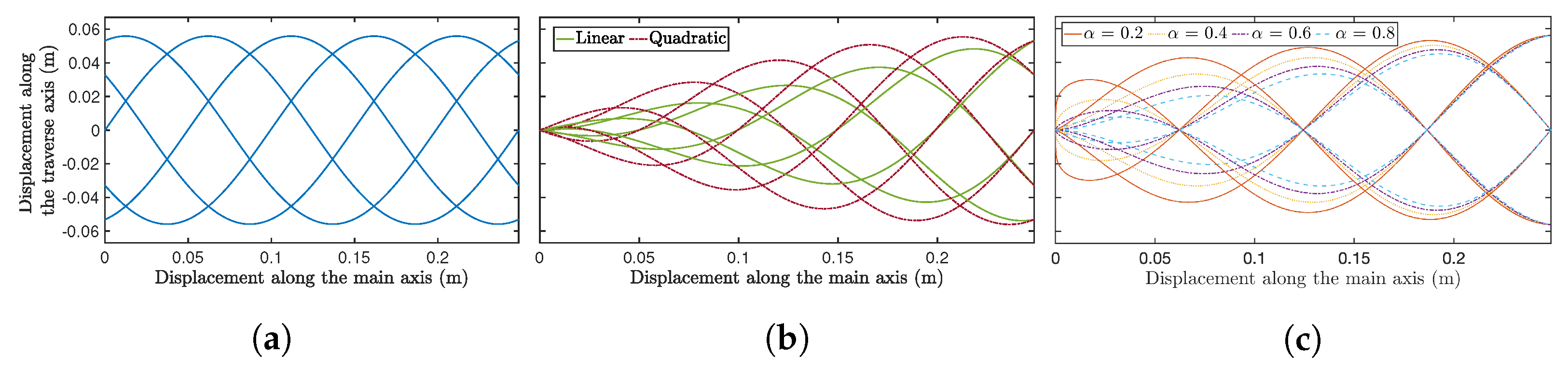
2.2. Waveforms
2.3. IPMC Technology
3. Swimming Robot
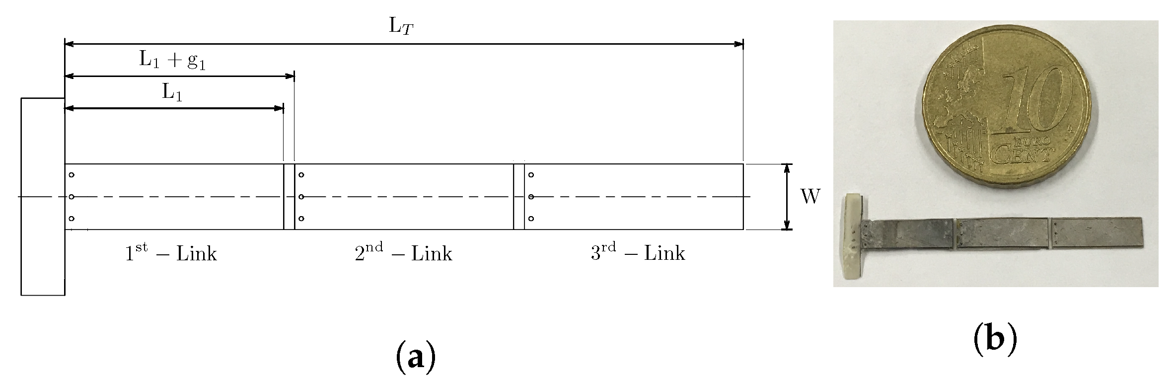
3.1. Robot Description
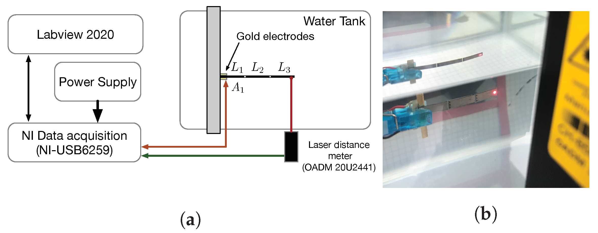
3.2. Experimental Setup
- A water tank, used as an environment since the ultimate goal of the swimming robot is to be able to swim in a fluid.
- A laser distance meter (OADM 20U2441), to measure the deflection of the links.
- Gold electrodes, attached by means of a clamp, to transmit the voltage from the supplier to the IPMC surface.
- A USB multifunction I/O data acquisition board of National Instruments (NI-USB6259), which is connected to a computer in which LabVIEW™ 2020 SP1 runs to collect the data and generate the desired excitation voltage.
- A power stage, to provide sufficient power to the actuator from a power DC supplier and the desired voltage indicated by the computer.
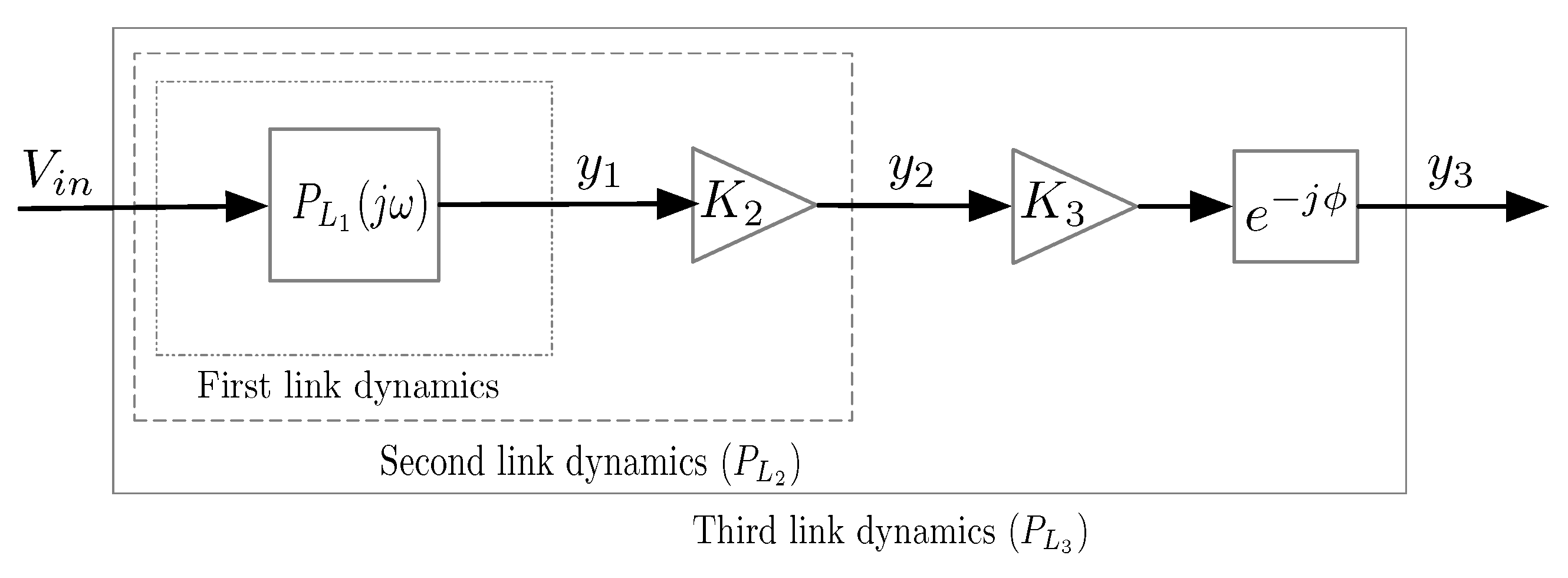
4. Robot Modeling
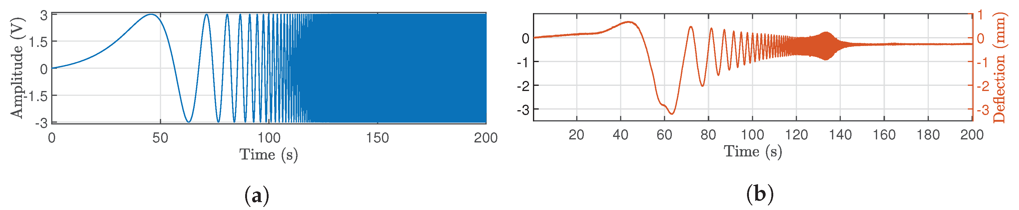
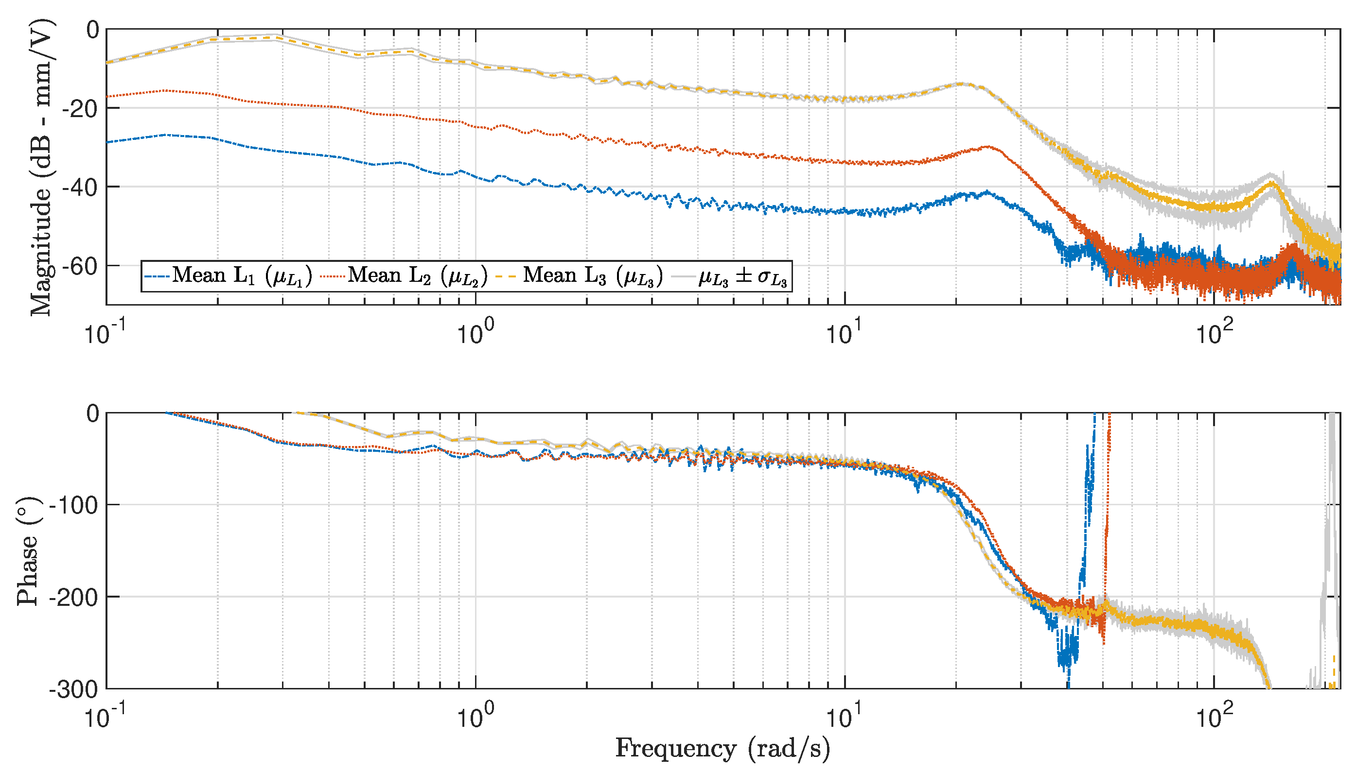
4.1. Measuring Frequency Responses
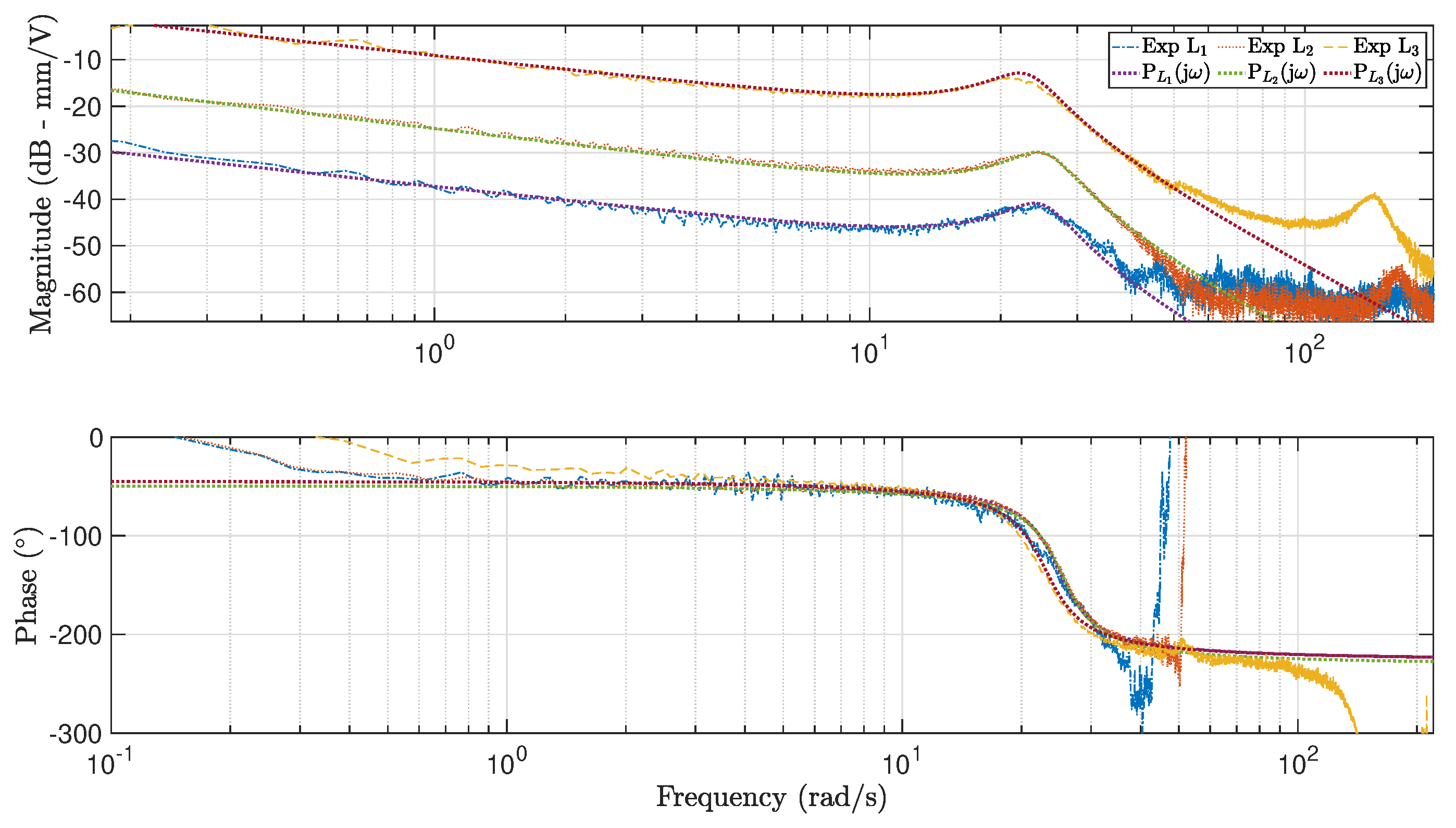
4.2. Dynamic Model Identification
4.3. Discussion of the Results
5. Robot Propulsion
5.1. Problem Formulation
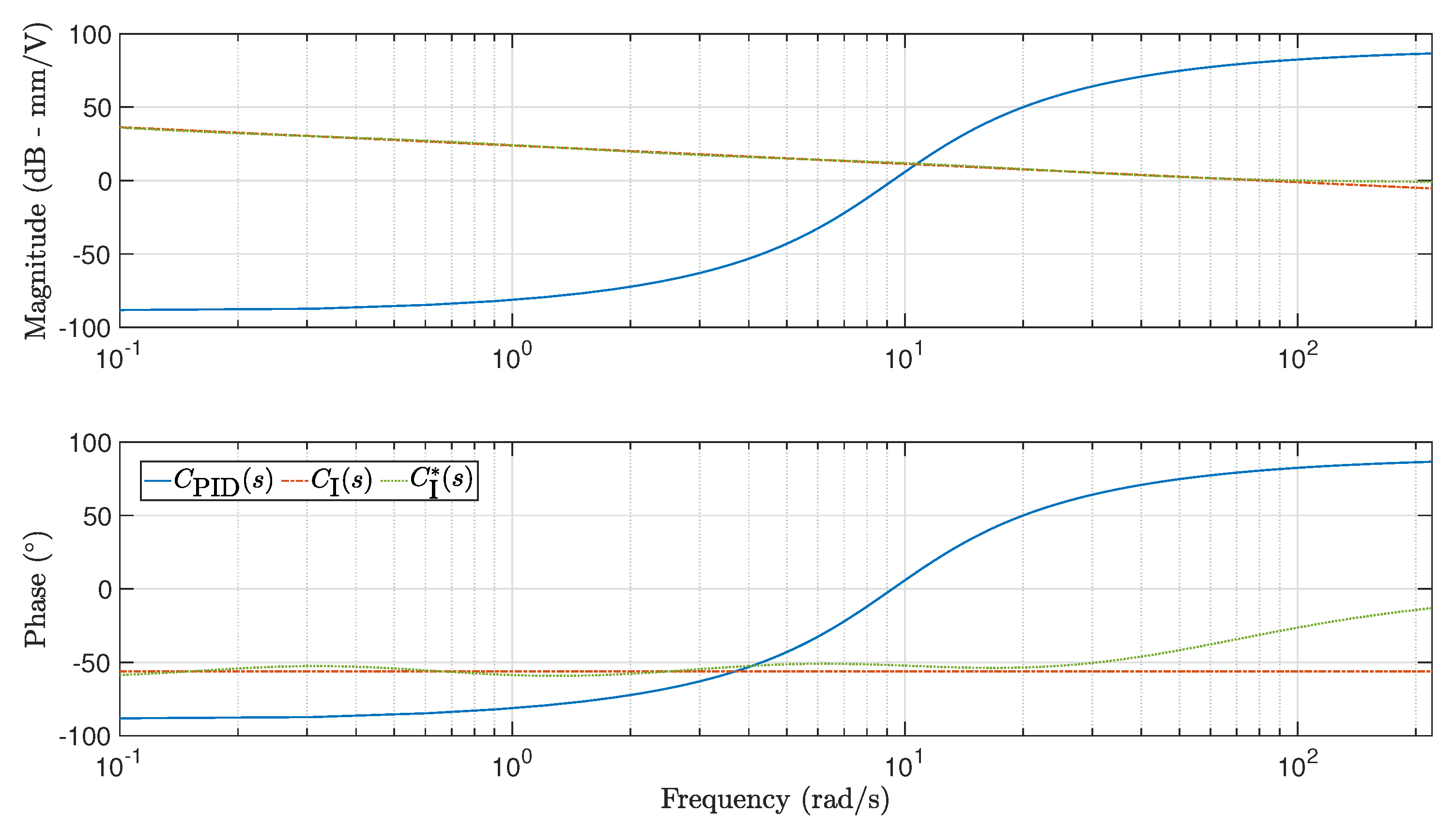
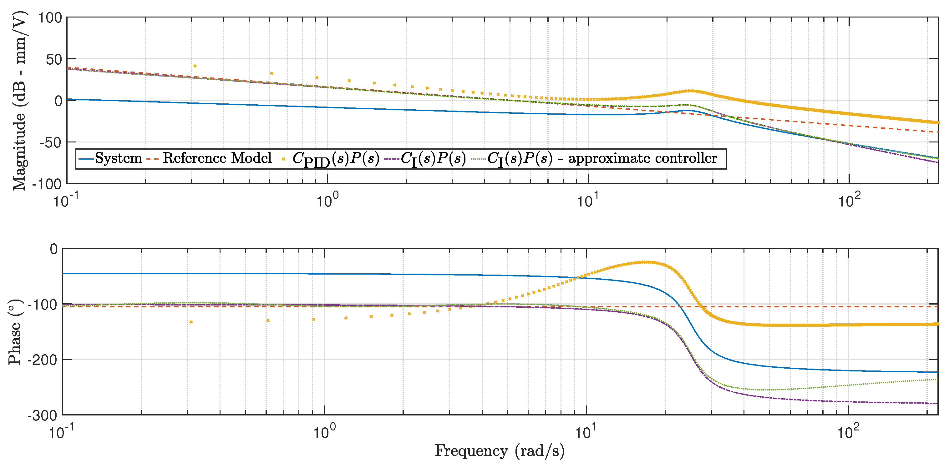
5.2. Control Design
- Gain crossover frequency: rad/s.
- Phase margin: .
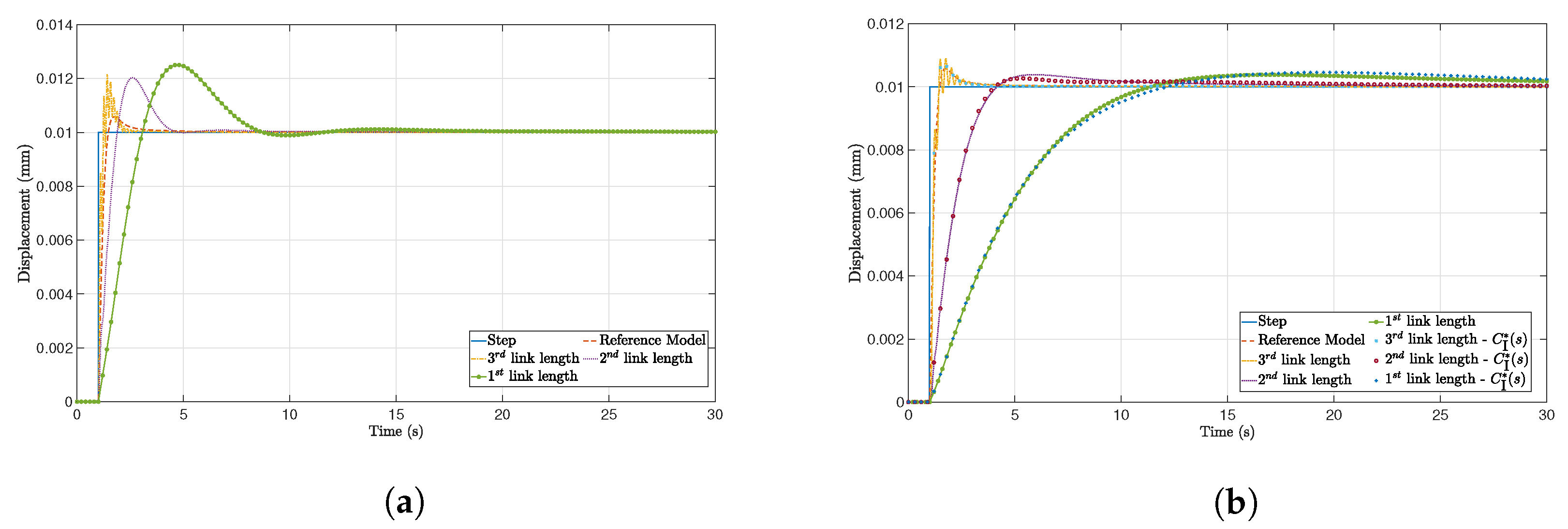
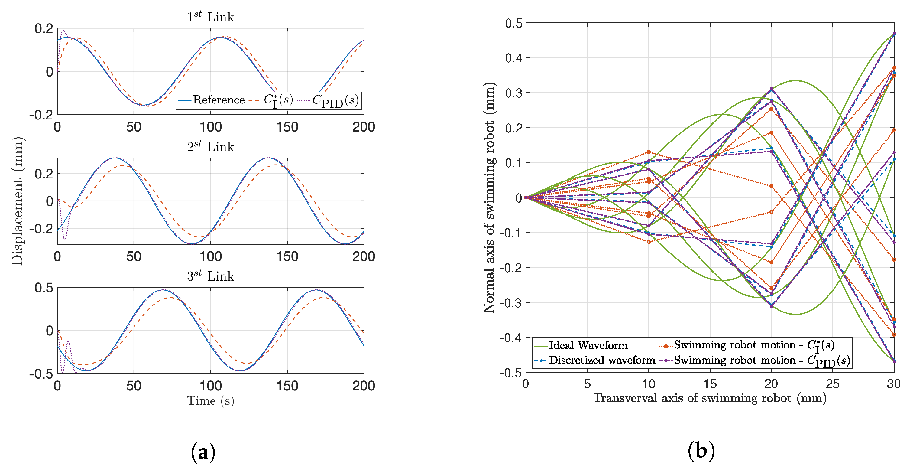
5.3. Motion Analysis
6. Conclusions
Author Contributions
Funding
Data Availability Statement
Acknowledgments
Conflicts of Interest
Abbreviations
| AEF | Artificial eukaryotic flagellum |
| IPMC | Ionic polymer-metal composite |
| PID | Proportional-integral-derivative |
| MAD | Mean absolute deviation |
| MD | Maximum deviation |
| MSE | Mean square error |
| R | Coefficient of determination |
| Re | Reynolds number |
| TADPOLE | Tiny artificial devices propelled on liquid environments |
References
- Sitti, M.; Ceylan, H.; Hu, W.; Giltinan, J.; Turan, M.; Yim, S.; Diller, E. Biomedical Applications of Untethered Mobile Milli/Microrobots. Proc. IEEE 2015, 103, 205–224. [Google Scholar] [CrossRef]
- Li, J.; Esteban-Fernández de Ávila, B.; Gao, W.; Zhang, L.; Wang, J. Micro/nanorobots for biomedicine: Delivery, surgery, sensing, and detoxification. Sci. Robot. 2017, 2, eaam6431. [Google Scholar] [CrossRef]
- Medina-Sánchez, M.; Xu, H.; Schmidt, O.G. Micro- and nano-motors: The new generation of drug carriers. Ther. Deliv. 2018, 9, 303–316. [Google Scholar] [CrossRef] [Green Version]
- Soto, F.; Wang, J.; Ahmed, R.; Demirci, U. Medical micro/nanorobots in precision medicine. Adv. Sci. 2020, 7, 2002203. [Google Scholar] [CrossRef]
- Arvidsson, R.; Hansen, S.F. Environmental and health risks of nanorobots: An early review. Environ. Sci. Nano 2020, 7, 2875–2886. [Google Scholar] [CrossRef]
- Wu, Z.; Chen, Y.; Mukasa, D.; Pak, O.S.; Gao, W. Medical micro/nanorobots in complex media. Chem. Soc. Rev. 2020, 49, 8088–8112. [Google Scholar] [CrossRef]
- Fu, S.; Wei, F.; Yin, C.; Yao, L.; Wang, Y. Biomimetic soft micro-swimmers: From actuation mechanisms to applications. Biomed. Microdevices 2021, 23, 6. [Google Scholar] [CrossRef]
- Sun, B.; Wood, G.; Miyashita, S. Milestones for autonomous in vivo microrobots in medical applications. Surgery 2021, 169, 755–758. [Google Scholar] [CrossRef]
- Jiang, J.; Yang, Z.; Ferreira, A.; Zhang, L. Control and autonomy of microrobots: Recent progress and perspective. Adv. Intell. Syst. 2022. [Google Scholar] [CrossRef]
- Shimoyama, I. Scaling in microrobots. In Proceedings of the 1995 IEEE/RSJ International Conference on Intelligent Robots and Systems. Human Robot Interaction and Cooperative Robots, Pittsburgh, PA, USA, 5–9 August 1995; Volume 2, pp. 208–211. [Google Scholar]
- Trimmer, W.; Jebens, R. Actuators for micro robots. In Proceedings of the 1989 IEEE International Conference on Robotics and Automation, Scottsdale, AZ, USA, 14–19 May 1989; pp. 1547–1548. [Google Scholar]
- Wautelet, M. Scaling laws in the macro-, micro-and nanoworlds. Eur. J. Phys. 2001, 22, 601–611. [Google Scholar] [CrossRef]
- Abbott, J.J.; Nagy, Z.; Beyeler, F.; Nelson, B.J. Robotics in the small, part I: Microbotics. IEEE Robot. Autom. Mag. 2007, 14, 92–103. [Google Scholar] [CrossRef]
- Lauga, E.; Powers, T.R. The hydrodynamics of swimming microorganisms. Rep. Prog. Phys. 2009, 72, 096601. [Google Scholar] [CrossRef]
- Diller, E.; Sitti, M. Micro-scale mobile robotics. Found. Trends Robot. 2013, 2, 143–259. [Google Scholar] [CrossRef]
- Sitti, M. Mobile Microrobotics; MIT Press: Cambridge, MA, USA, 2017. [Google Scholar]
- Wang, B.; Kostarelos, K.; Nelson, B.J.; Zhang, L. Trends in micro-/nanorobotics: Materials development, actuation, localization, and system integration for biomedical applications. Adv. Mater. 2021, 33, 2002047. [Google Scholar] [CrossRef]
- Lauga, E. Life at high deborah number. EPL (Europhys. Lett.) 2009, 86, 64001. [Google Scholar] [CrossRef]
- Raz, O.; Avron, J.E. Swimming, pumping and gliding at low Reynolds numbers. New J. Phys. 2007, 9, 437. [Google Scholar] [CrossRef]
- Hatton, R.L.; Choset, H. Geometric swimming at low and high Reynolds numbers. IEEE Trans. Robot. 2013, 29, 615–624. [Google Scholar] [CrossRef]
- Alouges, F.; DeSimone, A.; Giraldi, L.; Zoppello, M. Self-propulsion of slender micro-swimmers by curvature control: N-link swimmers. Int. J. Non-Linear Mech. 2013, 56, 132–141. [Google Scholar] [CrossRef]
- Wiezel, O.; Or, Y. Optimization and small-amplitude analysis of Purcell’s three-link microswimmer model. Proc. R. Soc. Math. Phys. Eng. Sci. 2016, 472, 20160425. [Google Scholar] [CrossRef] [Green Version]
- Kadam, S.; Joshi, K.; Gupta, N.; Katdare, P.; Banavar, R. Trajectory tracking using motion primitives for the Purcell’s swimmer. In Proceedings of the 2017 IEEE/RSJ International Conference on Intelligent Robots and Systems (IROS), Prague, Czech Republic, 27 September–1 October 2017; pp. 3246–3251. [Google Scholar]
- Kadam, S.; Banavar, R. Geometry of locomotion of the generalized Purcell’s swimmer: Modelling, controllability and motion primitives. IFAC J. Syst. Control 2018, 4, 7–16. [Google Scholar] [CrossRef]
- Kósa, G.; Jakab, P.; Hata, N.; Jólesz, F.; Neubach, Z.; Shoham, M.; Zaaroor, M.; Székely, G. Flagellar swimming for medical micro robots: Theory, experiments and application. In Proceedings of the 2nd IEEE RAS & EMBS International Conference on Biomedical Robotics and Biomechatronics (BioRob 2008), Scottsdale, Arizona, 19–22 October 2008; pp. 258–263. [Google Scholar]
- Abadi, A.; Kosa, G. Piezoelectric beam for intrabody propulsion controlled by embedded sensing. IEEE/ASME Trans. Mechatronics 2016, 21, 1528–1539. [Google Scholar] [CrossRef]
- Mancha, E.; Traver, J.E.; Tejado, I.; Prieto, J.; Vinagre, B.M.; Feliu, V. Artificial Flagellum Microrobot. Design and Simulation in COMSOL. In ROBOT 2017: Third Iberian Robotics Conference; Ollero, A., Sanfeliu, A., Montano, L., Lau, N., Cardeira, C., Eds.; Springer International Publishing: Cham, Switzerland, 2018; pp. 491–501. [Google Scholar]
- Traver, J.E.; Tejado, I.; Nuevo-Gallardo, C.; López, M.A.; Vinagre, B.M. Performance study of propulsion of N-link artificial eukaryotic flagellum swimming microrobot within a fractional order approach: From simulations to hardware-in-the-loop experiments. Eur. J. Control 2021, 58, 340–356. [Google Scholar] [CrossRef]
- Hariri, H.; Bernard, Y.; Razek, A. A traveling wave piezoelectric beam robot. Smart Mater. Struct. 2013, 23, 025013. [Google Scholar] [CrossRef]
- Prieto-Arranz, J.; Traver, J.E.; López, M.A.; Tejado, I.; Vinagre, B.M. Study in COMSOL of the generation of traveling waves in an AEF robot by piezoelectric actuation. In Proceedings of the XXXIX Jornadas de Automática, Badajoz, España, 5–7 September 2018; pp. 748–755. [Google Scholar]
- López, M.A.; Prieto, J.; Traver, J.E.; Tejado, I.; Vinagre, B.M.; Petrás, I. Testing non reciprocal motion of a swimming flexible small robot with single actuation. In Proceedings of the 19th International Carpathian Control Conference (ICCC 2018), Szilvásvárad, Hungary, 28–31 May 2018; pp. 312–317. [Google Scholar]
- Wang, T.; Ren, Z.; Hu, W.; Li, M.; Sitti, M. Effect of body stiffness distribution on larval fish–like efficient undulatory swimming. Sci. Adv. 2021, 7, eabf7364. [Google Scholar] [CrossRef]
- Dias, J.M.S. A Study on Bending Stiffness Characterization of Biohybrid Microrobots Using External Magnetic Actuation. Ph.D. Thesis, Universidade de Coimbra, Coimbra, Portugal, 2021. [Google Scholar]
- Shahinpoor, M.; Kim, K.J. Ionic polymer metal composites: IV industrial and medical applications. Smart Mater. Struct. 2004, 14, 197–214. [Google Scholar] [CrossRef]
- Shen, Q.; Wang, T.; Wen, L.; Liang, J. Modelling and fuzzy control of an efficient swimming ionic polymer-metal composite actuated robot. Int. J. Adv. Robot. Syst. 2013, 10, 350. [Google Scholar] [CrossRef]
- Hubbard, J.J.; Fleming, M.; Palmre, V.; Pugal, D.; Kim, K.J.; Leang, K.K. Monolithic IPMC fins for propulsion and maneuvering in bioinspired underwater robotics. IEEE J. Ocean. Eng. 2013, 39, 540–551. [Google Scholar] [CrossRef]
- Chen, Z.; Bart-Smith, H.; Tan, X. IPMC-actuated robotic fish. In Robot Fish; Springer: Berlin/Heidelberg, Germany, 2015; pp. 219–253. [Google Scholar]
- Chen, Z. A review on robotic fish enabled by ionic polymer–metal composite artificial muscles. Robot. Biomim. 2017, 4, 1–13. [Google Scholar] [CrossRef] [Green Version]
- Chen, Z.; Hou, P.; Ye, Z. Robotic fish propelled by a servo motor and ionic polymer-metal composite hybrid tail. J. Dyn. Syst. Meas. Control. 2019, 141, 071001. [Google Scholar] [CrossRef] [Green Version]
- Nemat-Nasser, S. Micromechanics of actuation of ionic polymer-metal composites. J. Appl. Phys. 2002, 92, 2899–2915. [Google Scholar] [CrossRef] [Green Version]
- Pugal, D. Physics Based Model of Ionic Polymer Metal Composite Electromechanical and Mechanoelectrical Transduction. Ph.D. Thesis, University of Nevada, Reno, NV, USA, 2012. [Google Scholar]
- Chen, Z.; Tan, X. A control-oriented and physics-based model for ionic polymer–metal composite actuators. IEEE/ASME Trans. Mechatronics 2008, 13, 519–529. [Google Scholar] [CrossRef]
- Caponetto, R.; Graziani, S.; Sapuppo, F.; Tomasello, V. An enhanced fractional order model of ionic polymer-metal composites actuator. Adv. Math. Phys. 2013, 2013, 717659. [Google Scholar] [CrossRef]
- Brennen, C.; Winet, H. Fluid mechanics of propulsion by cilia and flagella. Annu. Rev. Fluid Mech. 1977, 9, 339–398. [Google Scholar] [CrossRef] [Green Version]
- Happel, J.; Brenner, H. Low Reynolds Number Hydrodynamics: With Special Applications to Particulate Media, 1st ed.; Springer: Dordrecht, The Netherlands, 2012. [Google Scholar]
- Hinch, E. Hydrodynamics at low Reynolds numbers: A brief and elementary introduction. In Disorder and Mixing; Springer: Dordrecht, The Netherlands, 1988; pp. 43–56. [Google Scholar]
- Purcell, E.M. Life at low Reynolds number. Am. J. Phys. 1977, 45, 3–11. [Google Scholar] [CrossRef] [Green Version]
- Lauga, E.; Eloy, C. Shape of optimal active flagella. J. Fluid Mech. 2013, 730, R1. [Google Scholar] [CrossRef] [Green Version]
- Gray, J.; Hancock, G.J. The propulsion of sea-urchin spermatozoa. J. Exp. Biol. 1955, 32, 802–814. [Google Scholar] [CrossRef]
- Lighthill, M.J. Note on the swimming of slender fish. J. Fluid Mech. 1960, 9, 305–317. [Google Scholar] [CrossRef]
- Nemat-Nasser, S.; Li, J.Y. Electromechanical response of ionic polymer-metal composites. J. Appl. Phys. 2000, 87, 3321–3331. [Google Scholar] [CrossRef]
- Farinholt, K.M. Modeling and Characterization of Ionic Polymer Transducers for Sensing and Actuation. Ph.D. Thesis, Virginia Tech, Blacksburg, VA, USA, 2005. [Google Scholar]
- Caponetto, R.; Graziani, S.; Pappalardo, F.L.; Umana, E.; Xibilia, M.; Giamberardino, P.D. A scalable fractional model for IPMC actuator. In Proceedings of the 7th Vienna International Conference on Mathematical Modelling, Vienna, Austria, 5–7 February 2011; pp. 593–596. [Google Scholar]
- Caponetto, R.; Dongola, G.; Fortuna, L.; Graziani, S.; Strazzeri, S. A fractional model for IPMC actuators. In Proceedings of the 2008 IEEE Instrumentation and Measurement Technology Conference, Victoria, BC, Canada, 12–15 May 2008; pp. 2103–2107. [Google Scholar]
- Tejado, I.; Traver, J.E.; Prieto-Arranz, J.; López, M.Á.; Vinagre, B.M. Frequency domain based fractional order modeling of IPMC actuators for control. In Proceedings of the 2019 18th European Control Conference (ECC), Naples, Italy, 25–28 June 2019; pp. 4112–4117. [Google Scholar]
- Valério, D.; Sá da Costa, J. Ninteger: A fractional control toolbox for Matlab. In Proceedings of the 1st IFAC Workshop on Fractional Differentiation and its Applications, Bourdeaux, France, 19–21 July 2004; pp. 2103–2107. [Google Scholar]
- Barbosa, R.S.; Machado, J.A.T.; Ferreira, I.M. Tuning of PID controllers based on Bode’s ideal transfer function. Nonlinear Dyn. 2004, 38, 305–321. [Google Scholar] [CrossRef]
- Monje, C.A.; Chen, Y.; Vinagre, B.M.; Xue, D.; Feliu-Batlle, V. Fractional-Order Systems and Controls: Fundamentals and Applications, 1st ed.; Springer: London, UK, 2010. [Google Scholar]
- Arrieta, O.; Vilanova, R. Simple PID tuning rules with guaranteed Ms robustness achievement. IFAC Proc. Vol. 2011, 44, 12042–12047. [Google Scholar] [CrossRef] [Green Version]


| Parameter | Description | Value | Unit |
|---|---|---|---|
| L | Length of robot | 31 | mm |
| W | Width of robot | 3 | mm |
| h | Thickness | 250 | m |
| L | Length of actuator | 10 | mm |
| N | Number of links | 3 | - |
| g | Space between actuators | 500 | m |
| Model | () | () | () | ||
|---|---|---|---|---|---|
| First link | - | ||||
| - | |||||
| Second link | - | ||||
| - | |||||
| Third link | - | ||||
| - | |||||
| Model | J () | MSE () | MAD () | MD () | R | |
|---|---|---|---|---|---|---|
| First link | ||||||
| Second link | ||||||
| Third link | ||||||
| Parameter | Value | Description | Unit |
|---|---|---|---|
| 0 | Amplitude coefficient | m | |
| 200 | Amplitude coefficient | - | |
| 0 | Amplitude coefficient | 1/m | |
| f | Frequency | Hz | |
| 32 | Wavelength | mm |
| Link | IAE | ITAE | ||
|---|---|---|---|---|
| First link | 42 | |||
| Second link | ||||
| Third link | ||||
Publisher’s Note: MDPI stays neutral with regard to jurisdictional claims in published maps and institutional affiliations. |
© 2022 by the authors. Licensee MDPI, Basel, Switzerland. This article is an open access article distributed under the terms and conditions of the Creative Commons Attribution (CC BY) license (https://creativecommons.org/licenses/by/4.0/).
Share and Cite
Traver, J.E.; Nuevo-Gallardo, C.; Rodríguez, P.; Tejado, I.; Vinagre, B.M. Modeling and Control of IPMC-Based Artificial Eukaryotic Flagellum Swimming Robot: Distributed Actuation. Algorithms 2022, 15, 181. https://doi.org/10.3390/a15060181
Traver JE, Nuevo-Gallardo C, Rodríguez P, Tejado I, Vinagre BM. Modeling and Control of IPMC-Based Artificial Eukaryotic Flagellum Swimming Robot: Distributed Actuation. Algorithms. 2022; 15(6):181. https://doi.org/10.3390/a15060181
Chicago/Turabian StyleTraver, José Emilio, Cristina Nuevo-Gallardo, Paloma Rodríguez, Inés Tejado, and Blas M. Vinagre. 2022. "Modeling and Control of IPMC-Based Artificial Eukaryotic Flagellum Swimming Robot: Distributed Actuation" Algorithms 15, no. 6: 181. https://doi.org/10.3390/a15060181
APA StyleTraver, J. E., Nuevo-Gallardo, C., Rodríguez, P., Tejado, I., & Vinagre, B. M. (2022). Modeling and Control of IPMC-Based Artificial Eukaryotic Flagellum Swimming Robot: Distributed Actuation. Algorithms, 15(6), 181. https://doi.org/10.3390/a15060181