Article

Multi-Fidelity Gradient-Based Optimization for High-Dimensional Aeroelastic Configurations

1
Applied Mechanics Division, University of Dayton Research Institute, Dayton, OH 45469, USA
2
Air Force Research Laboratory, Aerospace Systems Directorate, Wright-Patterson Air Force Base, OH 45433, USA
3
NASA Langley Research Center, Aeroelasticity Branch, Hampton, VA 23666, USA
*
Author to whom correspondence should be addressed.
Algorithms 2022, 15(4), 131; https://doi.org/10.3390/a15040131
Submission received: 1 March 2022 / Revised: 2 April 2022 / Accepted: 13 April 2022 / Published: 16 April 2022

Abstract

:
The simultaneous optimization of aircraft shape and internal structural size for transonic flight is excessively costly. The analysis of the governing physics is expensive, in particular for highly flexible aircraft, and the search for optima using analysis samples can scale poorly with design space size. This paper has a two-fold purpose targeting the scalable reduction of analysis sampling. First, a new algorithm is explored for computing design derivatives by analytically linking objective definition, geometry differentiation, mesh construction, and analysis. The analytic computation of design derivatives enables the accurate use of more efficient gradient-based optimization methods. Second, the scalability of a multi-fidelity algorithm is assessed for optimization in high dimensions. This method leverages a multi-fidelity model during the optimization line search for further reduction of sampling costs. The multi-fidelity optimization is demonstrated for cases of aerodynamic and aeroelastic design considering both shape and structural sizing separately and in combination with design spaces ranging from 17 to 321 variables, which would be infeasible using typical, surrogate-based methods. The multi-fidelity optimization consistently led to a reduction in high-fidelity evaluations compared to single-fidelity optimization for the aerodynamic shape problems, but frequently resulted in a cost penalty for cases involving structural sizing. While the multi-fidelity optimizer was successfully applied to problems with hundreds of variables, the results underscore the importance of accurately computing gradients and motivate the extension of the approach to constrained optimization methods.

1. Introduction

The simultaneous optimization of aircraft shape and internal structural size for transonic flight is excessively costly and a barrier to the design of efficient and effective aircraft. Optimization cost scales poorly with the number of design parameters for many kinds of algorithms, rendering design impractical when many parameters are needed, e.g., to finely tailor wings aerodynamically and structurally for improved performance. Practical design optimization of high-fidelity, physics-based models in such high-dimensional spaces generally involves three ingredients: (1) the use of local, gradient-based optimization to avoid excessive function evaluations, (2) the use of analytic differentiation and adjoint variables to mitigate cost growth in the derivative calculation, and (3) the avoidance of cheaper-to-analyze surrogate models owing to the high cost of constructing such surrogates in high-dimensional spaces. This paper addresses methodological contributions impacting each of these ingredients.
The first contribution relates to the analytic calculation of design derivatives with adjoints, as parameterized by an analytical geometry description. The use of adjoint variables to compute derivatives of aerodynamic problems, and aeroelastic problems to a lesser extent, has been well studied [1,2]. The cost of computing derivatives with these variables has been seen to grow only very slowly with design space dimensionality. Martins and coworkers [3,4,5] developed aeroelastic design optimization frameworks for inviscid and viscous aerodynamics built on a custom analytic geometry, a vision that is extended here with a general-purpose, design model (CAPS) [6] and geometry engine (ESP) [7] framework supportive of multi-fidelity modeling [8]. This framework leverages two modern, fluid–structure-coupling procedures, FUNtoFEM [9,10] and MPHYS [11]. This paper verifies the design sensitivities produced by this framework for linear and nonlinear aerodynamics and assesses the scalability of their calculation with respect to design complexity. With ESP and CAPS being built on a true CAD kernel (OpenCASCADE [12]) and CAPS having automatic aerodynamic and structural meshing capabilities, the choice of software tools was motivated by the ability to compute sensitivities with respect to geometric parameters that are meaningful to designers (e.g., twist or airfoil thickness), as opposed to mesh-based shape parameterizations in the literature. At the same time, however, the approach also introduces challenges such as those associated with rebuilding geometries or regenerating unstructured grids throughout an optimization.
The second contribution is the quantification of the scalability of the multi-fidelity Broyden–Fletcher–Goldfarb–Shannon (MF-BFGS) algorithm developed by Bryson and Rumpfkeil [13,14]. As opposed to typical multi-fidelity optimization approaches optimizing over a sequence of surrogate models (of potentially high dimension), this algorithm leverages high-fidelity gradient information to determine an objective-reducing search direction and then utilizes a less expensive multi-fidelity model to reduce analysis costs in the line search. In a study of several analytical functions with up to 25 design variables [14], Bryson and Rumpfkeil found MF-BFGS to scale better than multi-fidelity trust region model management (TRMM) [15,16,17]. Bryson confirmed that the MF-BFGS method generally out-performed BFGS for an aeroelastic model of a tailless lambda-wing vehicle [13], but noted that the lack of analytic derivatives in that work made some optimization results difficult to interpret. As this model was also limited in complexity to seven design variables [13] (four aerodynamic and three structural), the authors in this paper sought a more richly parameterized and representative model, as well as analytical derivatives with which to assess MF-BFGS scalability.
To assess the scalability of analysis and optimization algorithms, the authors developed parametric aerodynamic and aeroelastic benchmark models constructed from the high-aspect-ratio, undeflected, Common Research Model configuration (uCRM-13.5) published by the University of Michigan MDO Lab [5]. The development of the parametric model supports an international effort chartered by the NATO Applied Vehicle Technology (AVT) Panel, which is investigating the application of multi-fidelity methods to military vehicle design [18]. This model, as well as the analysis methods applied by the AVT technical team are available for broad distribution.
The remaining portion of this paper is decomposed into three sections. Section 2 describes the multidisciplinary analysis and optimization methods of relevance to this paper, provides details regarding the construction of the aeroelastic uCRM model, and links the work to the literature. Section 3 summarizes analysis and optimization results, with an emphasis on scalability. The paper concludes in Section 4 with a results’ discussion along with some recommendations for future research.

2. Modeling and Analysis

To serve as a benchmark aircraft design problem, the present work considers the undeflected high-aspect-ratio variant [5] (developed by the University of Michigan’s MDO lab) of NASA’s Common Research Model (CRM). Beginning with an IGES CAD file (Available at https://mdolab.engin.umich.edu/wiki/ucrm, accessed on 17 January 2020), the fuselage was modeled in Engineering Sketch Pad (ESP) [7] as a series of ellipses along with several rows of spline coordinates for the wing hump region (which are normalized based on fuselage width and height and wing root chord and position). The tail is formed by lofting through NACA airfoil sections. To generate the wing’s planform shape, six high-level parameters (area, Yehudi break location, aspect ratio, leading edge sweep angle, inboard trailing edge angle, and taper ratio) are used to compute lower-level parameters such as chord lengths at the centerline, Yehudi break, and tip sections. Readers are referred to [18] for baseline values of the high-level wing parameters and the equations used to compute lower-level parameters.
Wing sectional shapes are parameterized using either NACA four-series airfoils or Kulfan [19,20] airfoils. Kulfan airfoil parameterizations, also known as Class-Shape Transformations (CSTs), unify shape and class functions so that critical parameters of an existing airfoil class (e.g., leading edge radius or trailing edge angle) can be controlled, while Bernstein polynomial shape functions provide more general geometric variations. To obtain the baseline geometry, each of the Kulfan parameterizations were fit to airfoil points from UM’s surface geometry via the Parametric Legacy Unstructured Geometry System (PLUGS) [21], a parametric geometry fitting capability in ESP. While any number of shape functions can be used, this work uses either 7 or 17 design variables per spanwise section, which produced maximum distances of the reference airfoil points to the generated geometry on the order of 0.5% and 0.1% of chord, respectively. Meanwhile, the inner mold line geometry is formed based on fractional spar locations at the wing–fuselage junction, Yehudi break, and wing tip, as well as the numbers of ribs in the wing and fuselage (5 from the centerline to wing–fuselage junction and 52 in the inboard and outboard sections). These inner and outer mold line ESP geometries, illustrated in Figure 1, are built within a pyCAPS [22] script, which can configure various analyses of rigid and aeroelastic physics at different levels of fidelity.
To assess a particular ESP geometry, pyCAPS provides an assortment of Analysis Interface Modules (AIMs), which prepare various aerodynamic or aeroelastic analyses based on the attributed geometry. This includes triangular, quadrilateral, or mixed mesh generation for shell structures, unstructured surface and volume meshing for nonlinear aerodynamic analyses (including surface grid sensitivities), and other input file generation for analyses that utilize linear aerodynamics (e.g., Nastran [23]). Through the use of several AIMs, basic analysis meshes and input files are generated for the parameterized ESP geometry. Pre- and post-processing external to pyCAPS are used for additional functionality. Details on particular aerodynamic or aeroelastic analyses are provided in Section 2.2.

2.1. Design Parameterizations

In the present work, a particular uCRM design can be described by several sets of design variables, including shape ( x s ), structural ( x t , i.e., shell thicknesses), and aerodynamic ( x a , e.g., cruise angle of attack). Different combinations of these parameter sets, which are all normalized by bounds to range from 0 and 1, were considered so that optimization cost trends can be assessed.
Two optional sets of shape design variables may be optimized in this work. Each set controls the sectional twist angles and airfoil shapes at the wing Yehudi and tip (where Yehudi refers to where the trailing edge sweep angle changes near mid-span), with one having 7 airfoil parameters per section, while the other has 17. The sets of initial parameters were both fit to UM’s reference geometry, with the higher-dimensional parameterization (and lower-dimensional one to a lesser extent) matching the reference geometry well at the two sections. Figure 2a illustrates these sections on the low-fidelity ESP geometry (which excludes the fuselage), with the inner mold line (IML) geometry shown for reference. In this figure, the two outboard wing cross-sections may be varied, while the two wing root sections and tail geometries remain fixed. Intermediate sectional shapes elsewhere in the wing are formed based on linear interpolation of the centerline, wing–fuselage junction, Yehudi, and tip airfoil sections. While an ESP model with many more airfoil sections has been developed and tested (containing ten additional cross-sections with around 200 design variables), it is not demonstrated in the present work. Furthermore, while the high-level planform parameters described in [18] may also be varied, they were held fixed in the present work.
In each airfoil section, the design variables comprise a chordwise row of control point z-coordinates above the airfoil, distances to a corresponding row of points below the airfoil, and one variable that influences the trailing edge angle (all of which are normalized by chord length). The lower bounds for the distance variables were set to −0.5, while the upper bounds were set to their initial values, thus avoiding designs that are thinner than the baseline design (approximately). When planform remains fixed, this approximately ensures that the wing volume does not decrease, allowing the same amount of room for fuel and other components (as well as the structure for rigid cases). Lower bounds for the upper set of points were set to 0.05. The upper bound for the top leading edge point was set to −0.05 minus the lower leading edge point’s initial value. This ensures that the lower leading edge point cannot go above −0.05, thus avoiding designs with sharp leading edges (which would presumably yield poor performance in off-design conditions). All other upper bounds for the top points were set to 0.5. Bounds for the trailing edge variable were −0.005 and 0.005. The sectional twist design variables at these two sections were allowed to vary from −3 to 6 degrees (initial values being 0.837972 and 4.612053 degrees, respectively).
The optional set of structural design variables includes the shell thickness of each rib, skin, and spar face, each comprising aluminum with a Young’s modulus of 6.9 × 10 10 Pa a Poisson’s ratio of 0.32, a density of 2700 kg/m3, and a yield stress of 2.76 × 10 8 Pa. Figure 2b illustrates these different faces in the IML geometry. Nodes at the centerline are assumed to be clamped (Neumann with zero displacement and rotation), while those at the wing–fuselage junction are pinned (Dirichlet with zero displacement). Consisting of 114 top and bottom skins, 58 ribs, and 111 spars, with arbitrary initial thicknesses of 0.02, 0.03, and 0.04 m, this set of design variables adds 283 design variables in total. When optimized, upper and lower bounds were set to 0.2 and 0.005 m, respectively. Note that inclusion of high-level planform parameters would lead to a slightly varying number of IML faces (and with it, structural design variables), as the IML’s rib faces always remain perpendicular to the wingbox’s leading edge. While not an issue in the present work (because planform variables were held fixed), it represents a challenge for this geometry parameterization approach when compared to the more standard use of Free-Form Definition (FFD) design variables. While the work of Brooks et al. [5] modeled stiffeners through a smeared stiffness approach, the present work currently neglects the presence of stiffeners. Masses of the engine, fuel, and other components were also neglected in the structural representation (although they appear in the objective and constraint functions).
Finally, the aerodynamic design variables consist of only flow angle of attack at cruise and, when considered, a pull-up maneuver. As discussed later in Section 2.4, flight altitude assumptions were held fixed, with angle of attack providing an additional means of satisfying constraints in the absence of control surfaces. Bounds were set to 0 and 6 degrees for cruise angle of attack, while the optional maneuver angle of attack was allowed to vary between 0 and 12 degrees.

2.2. Rigid and Aeroelastic Analysis with Design Sensitivities

Design optimization was carried out using analysis samples collected at two different levels of aerodynamic modeling fidelity: “low-fidelity” linear modeling via the Vortex Lattice Method (VLM) and “high-fidelity” nonlinear modeling via the Euler equations. Designs were carried out for a transonic cruise condition where VLM is informative, but not sufficiently accurate for preliminary design. At the target flight condition, steady responses were sought about either the rigid uCRM configuration (aerodynamic responses) or the flexible uCRM configuration (aeroelastic responses). For aeroelastic modeling, structural analysis was carried out using an open-source finite-element analysis capability common to both fidelity levels. The sensitivities of responses with respect to design parameters were computed in all cases through an adjoint formulation, with the exception of the low-fidelity (LF) rigid analysis model. Note that while Euler equations are more capable of modeling compressibility effects than VLM (with VLM unable to predict shocks), they still neglect viscous effects, which can lead to higher drag and phenomena such as flow separation. In order to predict these effects, Reynolds-Averaged Navier–Stokes (RANS) equations could be used, or the Euler-based loads could potentially be augmented with empirical drag relations. In this work, the former was not done because the simulation cost was estimated to be an order of magnitude higher than that of Euler; the latter was not done because of the lack of analytic sensitivities. Whether analytic sensitivities are available of course depends on the empirical drag’s formulation; however, methodologies such as that of Mason’s flat-plate-based FRICTION code [24] compute friction drag based on wetted area alone, yielding only a constant drag when the planform remains fixed. If the empirical relation depends on other parameters such as sectional lift, then analytic derivatives would likely require residual augmentation at the solver level of the CFD forward and reverse analyses.
Figure 3 illustrates the general process flow for assessing a particular design.
Initially, a design variable vector and fidelity level are fed into a Python-based function handle within a case recorder (which may evaluate the selected objective, inequality constraints, penalty-constrained objective, or any of their gradients). This is achieved through the use of a pyCAPS-based script, which loads the ESP geometry and adjusts the shape variables as needed, then rebuilds the OML geometry. Analysis pre-processing depending on geometry is handled via pyCAPS Analysis Interface Modules (AIMs), responsible for meshing and input generation. For optimization cases that only consider aerodynamics over a rigid wing, linear (low-fidelity) and nonlinear (high-fidelity) analyses were considered. For linear aerodynamic analyses, the AVL [26] pyCAPS AIM is used to generate a VLM representation of the wing and tail (with fuselage geometry excluded). When instead evaluating the design with nonlinear, CFD-based aerodynamics, the AFLR4 and AFLR3 [27] AIMs are used to generate unstructured meshes for the surface and volume, respectively, with pyCAPS also providing geometric sensitivities on the surface mesh through the use of the FUN3D [28] AIM.
For aeroelastic cases, the IML geometry is also rebuilt, with EGADS subsequently providing a structural mesh. The Nastran AIM then generates a Nastran input deck based on the specified structural boundary conditions and properties (including shell thicknesses, if varied by the optimizer). PyNastran [29] is used to edit the input deck before being loaded by the TACS [30] Bulk Data File (BDF) reader. For aeroelastic cases with linear aerodynamics, a mesh for a different VLM solver is also generated based on the sectional shapes given in the AVL input file. This separate VLM solver, a NASA-developed code made alongside the MPHYS effort, is analytically differentiated by hand, so when gradients are needed, the VLM mesh generation process is finite differenced before running the coupled adjoint analysis.
At this point, aerodynamic and structural meshes (if aeroelasticity is considered) are available. For rigid analyses, the fluid solver is then run. For aeroelastic cases with VLM-based aerodynamics, an MPHYS driver is used to obtain the static aeroelastic solution using the two grids and various inputs such as atmospheric conditions and geometric sensitivities (when evaluating gradients). For CFD-based aeroelastic cases, the same approach is taken with a FUNtoFEM driver. In the end, the rigid or aeroelastic analyses provide low-level quantities of interest such as force and moment coefficients, which will later be used in higher-level objective and constraint functions (with chain-rule derivatives computed as needed).
A summary of the analysis levels and associated software tools is given in Table 1. Further details regarding the tools implementing these analyses are provided in Section 2.2.1 and Section 2.2.2.

2.2.1. Rigid Aerodynamic Analysis

Aerodynamic solutions of the rigid uCRM configuration in steady, transonic flight are computed at two fidelity levels, as outlined in Table 1. The LF solution is computed with a widely distributed, linear, VLM methodology known as Athena Vortex Lattice (AVL), developed by Drela and Youngren [26]. Drag estimates produced by AVL are corrected for wave drag using the Korn equation, applied in stripwise fashion using an aerodynamic technology factor of 0.87 [31]. Since AVL is not analytically differentiated, the sensitivities of the computed aerodynamic quantities with respect to the design parameters are computed with one-sided finite differences using an appropriately chosen step size (a relatively large normalized step size of 0.1, on account of AVL’s low decimal precision). While the cost of computing these sensitivities grows linearly with the number of design variables, the overall cost is small owing to the speed of LF analysis and is not considered a bottleneck for the configuration studied herein. Furthermore, for aeroelastic analysis, a different VLM formulation is used that is analytically differentiated.
Higher-fidelity aerodynamic solutions are computed with FUN3D [28], which can solve the steady or unsteady Euler or Navier–Stokes equations on unstructured meshes. The benefit of FUN3D over other available solvers is that flow equations are analytically differentiated internally using the discrete adjoint approach, which permits the scalable and accurate computation of design derivatives in a manner consistent with the discretized governing equations.
An arbitrary design objective (or constraint function) f f ( D , Q a , X g ) is assumed to depend on the set of design variables, D x s , x a T , the aerodynamic state variables, Q a , and the computational mesh, X g . For gradient-based optimization, the variation of J with D is required, where Q a and X g are dependent on D . Following the adjoint approach of Nielsen and Park [32], the total derivative of f at a known rigid solution is expressed as
d J d D = f D + Λ a T R a D Λ g T X g D surface ,
where J J ( D , Q a , X g , Λ a , Λ g ) = f ( D , Q a , X g ) + Λ a T R a + Λ g T R g is a Lagrangian function, R a ( D , Q a , X g ) is the residual array of the discretized aerodynamic equations, R g ( X g , X g surface ) is the residual array of the discretized mesh deformation equations, and Λ a and Λ g are arrays of adjoint variables satisfying:
R a Q a T Λ a = f Q a
and
K T Λ g = f X g R a X g T Λ a .
Equations (1) and (3) assume FUN3D’s internal linear mesh deformation equation, R g K X g X g surface = 0 , where K is a linear matrix. By computing Λ a and Λ g for a fixed number of design objectives (or constraint functions), design derivatives at known rigid solutions can be computed from Equation (1) in a manner whose cost remains small compared to the cost of computing a steady solution, even when the number of design parameters becomes large.

2.2.2. Aeroelastic Analysis

To obtain aeroelastic responses and adjoint derivatives, the TACS [30] structural solver is coupled to either FUN3D or a linear Vortex Lattice Method (VLM) augmented with an empirical drag build-up. Currently, VLM-based coupling is performed through the use of MPHYS [11], a collection of helper Python classes, which seeks to standardize, create, and verify aerostructure couplings and derivatives in OpenMDAO [33] and is developed by NASA, the University of Michigan, and Georgia Tech. Higher-fidelity coupling is performed using FUNtoFEM [9,10], an effort led by NASA, AFRL, and Georgia Tech.
For comparison, aeroelastic solutions of the baseline uCRM configuration (using the 7-DoF airfoil parameterization) are computed with the LF and HF methodologies for steady, transonic cruise (conditions are listed later in Section 2.2.2). Residuals of both analyses dropped by roughly 8 orders of magnitude in 15 and 400 solver iterations for the LF and HF methods, respectively (where the HF solver solves one flow iteration per coupling iteration). The resulting lift and drag coefficients were 0.48836 and 0.022951 for LF analysis, respectively, compared to 0.49733 and 0.020454 for HF, yielding differences of −1.8037% and +12.2086%. Sample pressure and stress contours of the Euler- and VLM-based analyses are shown in Figure 4. For clarity, the Euler- and VLM-based deflections are overlaid on one another in Figure 5. It is evident that the Euler analysis generates a slightly larger lift and generates somewhat larger aeroelastic deformations.
To avoid repetition, the description of aeroelastic analysis herein is limited to a review of the HF methodology composed of FUN3D, TACS, FUNtoFEM, and CAPS/ESP. The methodology of computing aeroelastic solutions and design derivatives with these methods was developed by Kiviaho et al. [9] and Jacobson et al. [10,34]. Steady aeroelastic solutions (the so-called primal problem) are iteratively computed with an under-relaxed nonlinear block Gauss–Seidel (BGS) method until residual convergence, treating aerodynamic, structural dynamic, mesh, and load/deformation residual equation sets as separate blocks; see Algorithm 1 in [9]. FUN3D is used to step the solution of the aerodynamic and mesh blocks (residuals R a and R g , respectively); TACS is used to step the structural dynamic block (residual R s ); FUNtoFEM is used to drive the BGS method and execute the load and displacement transfers using the MELD transfer scheme (residuals R f , R l , R d , with subscripts “l” and “f” denoting distributed and integrated loads, respectively). Finally, CAPS/ESP is used to create the meshed geometry shared by these software components.
To analytically obtain design derivatives, an adjoint problem corresponding to the BGS scheme is solved for each cost function f (which, as in the rigid analysis described above, may include lift, drag, pitching moment, or an aggregated stress response; the gradients of the structural mass and center of gravity were assumed to be uncoupled). Following Jacobson et al. [9,10,34], specific coupled adjoint equations are formed by the introduction of a Lagrangian, with the notation consistent with that of rigid analysis:
J = f + Λ a T R a + Λ g T R g + Λ s T R s + Λ f T R f + Λ l T R l + Λ d T R d .
Adjoint variables are computed by FUNtoFEM using a linear BGS scheme involving a blocked system matrix composed of transposed matrices (as suggested by Equation (3), which features the transpose of the linearized aerodynamic equations); see Algorithm 2 in [9]. One set of adjoint variables is computed at each point of the design space, and with this set, the design derivatives are computed from [9]:
d J d D = f D + Λ a T R a D + Λ g T R g D + Λ s T R s D + Λ f T R f D + Λ l T R l D + Λ d T R d D .
For the shape variables (differentiation with respect to Yehudi twist is examined below), the derivatives are computed through a chaining of physical and geometric sensitivities (i.e., the functional of interest with respect to mesh and the mesh with respect to the design variables). Mesh quantities are broken into two sets, aerodynamic ( X ga ) and structural ( X gs ) (with X ga being aerodynamic surface nodes and X gs being all structural nodes), leading to the general expression for the design derivatives [9]:
d J d D = f X ga + Λ a T R a X ga + Λ g T R g X ga + Λ s T R s X ga + Λ f T R f X ga + Λ l T R l X ga + Λ d T R d X ga ] X ga D + [ f X gs + Λ a T R a X gs + Λ g T R g X gs + Λ s T R s X gs + Λ f T R f X gs + Λ l T R l X gs + Λ d T R d X gs ] X gs D .
The dot product of the adjoint-computed surface vector with geometric sensitivities (i.e., the sensitivities of the aerodynamic surface and structural grid coordinates with respect to a shape design variable, otherwise referred to here as design velocities) then provides the gradient of f with respect to a particular design variable. Here, structural design velocities were neglected for both LF and HF analysis due to current limitations with ESP and with the assumption that they are small compared to aerodynamic design velocities (see the verification for the baseline analysis case presented in Section 2.3), thus providing:
d J d D = f X ga + Λ a T R a X ga + Λ g T R g X ga + Λ s T R s X ga + Λ f T R f X ga + Λ l T R l X ga + Λ d T R d X ga ] X ga D
It should also be noted that for aeroelastic analyses in cruise, one primal and three adjoint solutions are computed; when also considering a maneuver scenario, two primal and five adjoint solutions are computed.
To illustrate how shape derivatives are computed with FUNtoFEM and ESP, components of the HF sensitivity analysis are displayed in Figure 6 for the objective of the lift coefficient and the Yehudi twist parameter. Figure 6a shows the chained, composite adjoint array (the expression in brackets in Equation (7)) for wing lower (left) and upper (right) surfaces, while the top three parts of Figure 6b show the aerodynamic design velocity components X ga / D surface . The elements of the resulting dot product between adjoint variables and design velocity components are shown at the bottom of Figure 6b.

2.3. Accuracy and Cost of Derivative Calculations

The adjoint-based process for computing design derivatives was verified by comparison of analytically computed derivatives to first-order-accurate, forward finite differences for the baseline cruise case. The lift coefficient was selected as the objective, and derivatives with respect to the Yehudi twist angle and the thickness of an arbitrarily selected structural element, t 42 (the 4th trailing edge spar outboard from the wing–fuselage junction), were compared. Step sizes of 0.01 and 0.0001 were selected for the shape and sizing variables; to settle on these values, increasingly small step sizes were tested until the gradients roughly matched. Table 2 shows the resulting lift coefficient derivatives (an analytic derivative is not available for the low-fidelity rigid case). While optimizations regenerate the aerodynamic grids for each new design, the aerodynamic grids here were modified by smoothly mapping the initial mesh onto the perturbed geometry. For aeroelastic cases, the perturbed structural grids were generated by rebuilding and remeshing the IML geometry.
For both models, gradients with respect to structural thicknesses (as well as angles of attack) were observed to be more precise when compared to shape derivatives for the flexible vehicle. Because the shape derivative was found to be more accurate for the rigid case, the increased error for the flexible case may in part be due to the neglect of structural design velocities. To help estimate how large this source of error may be, the HF aeroelastic model was also perturbed while fixing the IML’s geometry and mesh. This resulted in a finite-difference gradient of 0.05409046, yielding an adjoint error of −0.0768%, thus suggesting the structural shape gradient term in Equation (6) changes the gradient by around −0.2796%. However, note that a mainly structural response such as an aggregated stress constraint may have a larger discrepancy when compared to an aerodynamic load such as the lift coefficient. For the LF model, imprecise geometric sensitivities are likely a larger contributing factor. Nonetheless, the analytic derivatives compared reasonably well to finite differences.
The computational efficiency of computing derivatives is next assessed for LF and HF analyses using parameterizations of differing dimensionality. It was observed for the most computationally demanding analysis case, HF aeroelastic analysis, that computational time scales slowly with the size of the design space. Results were measured in terms of wall-clock time. Each HF run utilized 32 CPUs and involved 600 steps (or reaching a consistent residual of 1 × 10 10 for rigid runs); parallelism was exploited where possible. The LF analysis typically involved 15 steps, but in some cases required 30 steps to achieve convergence. Although the LF aeroelastic model is capable of parallel execution, 1 CPU was used. With 41 chordwise nodes throughout (clustered near leading and trailing edges), the LF aerodynamic meshes contained 2378 nodes and 2240 elements on the wing and 902 nodes and 800 elements on the tail. The (somewhat coarse) HF aerodynamic mesh averaged roughly 350 K nodes and 2 M cells, respectively. Structural meshes for both fidelities consisted of around 25 K nodes and 27 K CQUAD4 elements.
Figure 7 shows the mean wall-clock times required to prepare and run the models versus the number of shape design variables for several parameterizations.
For the LF rigid model, both the preparation and run times scaled linearly with the number of design variables, since the derivatives were computed with finite differences. Note, however, that the VLM used for the aeroelastic analysis, which is analytically differentiated, could be used instead; this has not yet been implemented and is a topic of future work. Because the other models obtain gradients through adjoint solvers, run times only depend weakly on the number of design variables. Note that for the sizing-only cases in Figure 7d (i.e., cases with fewer than 300 design variables), model preparation must only be performed once if the pyCAPS instance is retained in memory. Building the IML and OML geometries and generating the aerodynamic and structural meshes made up almost all of preparation time, while rewriting the TACS input deck with different property cards was cheap in comparison.
Case preparation times did, however, increase with dimensionality. While this was most significant for the LF aeroelastic model, the finite differencing process to obtain geometric sensitivities can be carried out in parallel. The case preparation time was also significant for the rigid high-fidelity model. While other airfoil parameterizations in ESP (e.g., PARSEC or NACA) are fully differentiated, Kulfan primitives still rely on internal finite differencing to obtain aerodynamic design velocities, which slows down the process marginally. A more significant increase in sensitivity calculation time was caused by the union of the fuselage and wing, as well as how the fuselage hump is formed (through splining with sketch primitives, which are also not differentiated). For instance, for the highest-dimensional rigid model, the wing and tail alone required 1.7 min for building the geometry, meshing, and computing surface mesh sensitivities. When done with the fuselage included, this required 5.4 and 7.3 min when excluding and including the fuselage hump, respectively. The structure’s wingbox also uses sketch primitives and a number of intersections and unions, so further improvements in sensitivity speeds would likely be required before including structural design velocities in the aeroelastic adjoint gradients. Fortunately, the case preparation times were insignificant for the HF aeroelastic case (when excluding structural design velocities) due to the much greater run times. A similar situation would be expected for the RANS equations, which would require finer grids and longer run times than for Euler.

2.4. Multi-Fidelity Design Benchmark Problems

Following the work of Brooks et al. [5], the present design problems focus on fuel burn minimization with lift, moment, and stress constraints with the design specifications listed in Table 3. The specifications are largely based on those of Brooks et al., with the exception of takeoff and landing fuel burn percentages, which are based on the Transonic Truss-Braced Wing (TTBW) work at Virginia Tech and NASA [31]. In addition, due to how the pitching moment was constrained in this work, the engine diameter and mass, as well as center of gravity locations of fixed and payload masses were also introduced. This was mainly done due to how widely the planform may vary with certain shape parameterizations; for instance, while the engine’s mass is not modeled in the structural analysis, it is at least presumed to move with the planform geometry (wing Yehudi’s leading edge point), with similar assumptions for fuel weight (inboard wing’s centroid).

Objective and Inequality Constraint Functions

The primary responses of interest (and their total derivatives) used in optimization are fuel burn, load factor, and pitching moment at the beginning of cruise, as well as stress and load factor constraints at an optional pull-up maneuver. Total fuel burn on a typical mission, F B total , is computed as
F B total = F B takeoff + F B cruise + F B landing
where takeoff and landing fuel burns are computed as percentages of the current weight, while cruise fuel burn is computed using the Breguet range equation (with freestream velocity V in nmi/hr to match units of range and SFC):
F B landing = L G W × 100 100 % FB , landing 1 ,
F B cruise = L G W + F B landing × exp R a n g e × S F C × C D , c r u i s e V , c r u i s e × C L , c r u i s e 1 ,
and
F B takeoff = L G W + F B landing + F B cruise × 100 100 % FB , takeoff 1 ,
where landing gross weight ( L G W ) is a factor of structural and fixed weights,
L G W = W struct + W fixed + W engine + W payload + W fuel , reserve .
This yields a maximum takeoff weight ( M T O W ) of
M T O W = L G W + F B total .
The load factor at the beginning of cruise can then be computed as
η cruise = L i f t cruise M T O W F B takeoff
whereas the load factor in the maneuver condition (when including structural sizing variables) is computed as
η maneuver = L i f t maneuver M T O W
The pitching moment at the start of cruise is computed as the sum of several components about the nose,
M total = M aero + M thrust + M fuel mass + M struct mass + M engine mass + M fixed mass
where the aerodynamic moment is computed by the VLM or CFD aerodynamic models,
M aero = 1 2 ρ , c r u i s e V , c r u i s e 2 b ref S ref C M y , c r u i s e ,
and the pitching moment from thrust is computed using cruise drag force (thus, assuming drag equals thrust) and presumed nacelle dimensions,
M thrust = D r a g cruise × z nose z C p , engine ,
with the engine’s center of thrust ( z C p , engine ) being positioned one-half the nacelle’s diameter below the wing’s Yehudi leading edge point. The moment from fuel weight M fuel mass is computed as
M fuel mass = η cruise × M T O W F B takeoff × x C g , fuel x nose ,
with the fuel’s center of mass ( x C g , fuel ) presumed to reside at the centroid of the wing’s inboard section. The moment from structural weight is computed based on the cruise load factor and the structure’s mass and center of gravity (which remain fixed for rigid optimization cases and vary for aeroelastic cases). The moment from the engine’s mass is computed using the cruise load factor and a presumed engine mass, with the engine’s center of gravity assumed to reside at the wing Yehudi’s leading edge x-coordinate. The moment from the remaining mass ( M fixed mass ), including fixed and payload masses, is computed based on the cruise load factor, presumed masses, and a somewhat arbitrarily chosen center of gravity coordinate, which was chosen such that the rigid baseline geometry (with arbitrary structural thicknesses) was trimmed. Finally, when designing structural gauges, an aggregated stress constraint is computed by TACS using the discrete Kreisselmeier–Steinhauser (KS) [35,36] formulation with a weighting of 50.
For design optimization, the objective function is total fuel burn normalized by 80,000 kg,
f = F B total 80 , 000
so that it is roughly on the order of 1. Among the inequality constraints g 0 , the first constraint is the cruise load factor constraint,
g 1 = 1 η cruise ,
which ensures that lift is greater than or equal to weight at the beginning of cruise. To ensure a total pitching moment of approximately zero at the start of cruise, two additional constraints are enforced,
g 2 = M total L e n g t h fuselage 0.01
and
g 3 = M total L e n g t h fuselage 0.01 ,
with the total moment being (somewhat arbitrarily) normalized by fuselage length to make it on the order of 10 and a downward shift of 0.01 to help avoid optimization convergence issues. When including the structural sizing variables, maneuver load factor, and KS stress constraints,
g 4 = 2.5 η maneuver
and
g 5 = K S 1 / 1.5 ,
are included so that the aggregated function (with a factor of safety of 1.5) is enforced at a 2.5 g pull-up maneuver. Note that all responses and total derivatives can be computed analytically using 2 forward solves (cruise, maneuver) and 5 adjoint solves (lift, drag, and pitching moment at cruise and lift and stress at maneuver), in addition to structural mass and center of gravity sensitivities (computed without adjoint solves). When not including structural sizing, this would require 1 forward solve and 3 adjoint solves.
It should be noted that, in reality, treating the load factor and moment constraints (i.e., g 2 g 4 ) as equality constraints may be of greater interest. In the present work, this was not done for several reasons. The primary reason is to avoid potential difficulties by an optimizer. In addition, the optimum should, in theory, yield active load factor constraints because of tradeoffs between aerodynamic performance and feasibility (for example, fuel burn and load factor tend to trend in the same direction with increasing angle of attack). Finally, if atmospheric conditions remain fixed, the load factor and moment will change throughout a mission as fuel is expended, so enforcing equality constraints would still only yield feasibility at one point in the mission.
Although the model tool chain was set up to handle inequality constraints directly, the BFGS-based multi-fidelity optimizer in this work is inherently an unconstrained optimization method. As such, when using that particular optimizer, quadratic penalty functions are used to enforce the inequality constraints as
f penalty = f + P factor × max g + P offset , 0 2 ,
where each constraint’s penalty factor and offset (to help avoid slightly violated constraints) were somewhat arbitrarily set based on estimated values. The resulting values are given in Table 4. Note that this incurs an additional offset for the moment constraint; serving different purposes, this simply ensures that an optimizer with direct constraint handling would enforce a similar constraint as a penalty-constrained one.

2.5. Multi-Fidelity, Gradient-Based Design Optimization

While global, derivative-free optimization methods such as surrogate-based or genetic algorithms are well-suited for multimodal, noisy, or non-differentiable design problems, gradient-based methods are ultimately needed when optimizing an expensive function with tens of design variables or more. For such cases, methods based on BFGS or Sequential Quadratic Programming (SQP) tend to be some of the most efficient [37], with SQP having the advantage of direct constraint handling. Such methods scale reasonably well with the number of design variables, but may still require upwards of 100 high-fidelity evaluations to reach an optimum. The use of multi-fidelity methods therefore becomes attractive if they have the potential to reduce the total number of high-fidelity evaluations required.
The multi-fidelity BFGS (MF-BFGS) method presented in [13,14] (previously termed the unified multi-fidelity or multi-fidelity quasi-Newton) is used to demonstrate gradient-based, multi-fidelity, aero-structural design optimization. The approach is an unconstrained optimization method similar to the standard, single-fidelity BFGS quasi-Newton method, necessitating the constraint penalty function. Extension of the multi-fidelity concepts to constrained optimization is an area for future research. Figure 8 provides an XDSM diagram outlining the multi-fidelity optimization process.
A goal of this approach is to improve the scalability of multi-fidelity optimization with respect to the number of design variables. Popular methods such as Trust Region Model Management (TRMM) [15,16,17] and efficient global optimization [38] rely on building accurate surrogate models (or surrogate corrections to a lower-fidelity analysis) over as large a region as possible. Consequently, these approaches suffer from the curse of dimensionality inherent to the underlying surrogate methods. In contrast, the MF-BFGS method leverages the concept of an expected point (the result of a bound-constrained quadratic sub-problem, Step 2) to construct a localized, two-point correction (Step 4) focused along the search direction. MF-BFGS leverages high-fidelity gradient information (Step 8) to construct an approximate Hessian (Step 1) and find an objective-reducing search direction. While the method uses high-fidelity gradients and search directions, the line search (Step 5) implements corrected low-fidelity data (Step 6) with the goal of reducing overall cost. Another advantage of approximating the Hessian with high-fidelity gradients is that if multi-fidelity optimization fails to make progress, the process can revert to high-fidelity optimization (Step 10) with no loss of data.
The numerical implementation of MF-BFGS is a Python wrapper around a slight modification of Nocedal’s Limited-memory, Bound-constrained BFGS software (L-BFGS-B) [39,40], compiled using the F2Py Fortran-to-Python compiler. The modifications were required to break the iteration and manage the use of high- and multi-fidelity data within the optimization, as well as to manipulate the design data in the case of rejected steps. For a single fidelity of analysis, the method reduces to the original L-BFGS-B implementation. The algorithm minimizes a quadratic approximate model at the k th iterate, m ( k ) D [39],
m ( k ) D = f h D ( k ) + f h ( k ) T D D ( k ) + 1 2 D D ( k ) T H ( k ) D D ( k ) ,
where the objective function and its gradient, f h and f h , are evaluated using the high-fidelity analysis, and the positive definite approximate Hessian H is approximated via the BFGS update over a series of steps, as described in [39,40] (omitted here for conciseness). With the search direction defined by the the step minimizing this sub-problem, subject to the side constraints on the design variables, a line search may be performed using either the high-fidelity function or a multi-fidelity correction to the low-fidelity function. The optimization begins with the multi-fidelity line search and reverts to high-fidelity once the gradient norm is reduced to a user-selected level or the multi-fidelity trust region becomes too small to make progress, also defined by the user. In this work, the transition criteria are a gradient norm of 1 × 10 3 or a trust region smaller than 0.001 (for normalized variables) for three successive iterations, which is aggressive in attempting to find a small trust region where the multi-fidelity model is sufficiently accurate rather than resorting to high-fidelity optimization. The reader is reminded here that the gradient and approximate Hessian always use the high-fidelity function; thus, the transition to single-fidelity optimization occurs as if the high-fidelity function was used from the start.
While any method that enforces first-order consistency (i.e., function value and gradients) at the current design point may be used to construct the low-fidelity correction function, this and prior aero-structural design applications [41] implement the gradient-enhanced, Multi-Fidelity Polynomial Chaos (MFPC) implementation presented in [13,42]. While polynomial chaos itself suffers from the curse of dimensionality, similar to other surrogate modeling techniques, here, the polynomials are limited to first order to ameliorate cost growth. Using both the high- and low-fidelity function and gradient information at two points (the selection of points will be explained momentarily), first-order additive and multiplicative corrective terms are computed in the form
f h D f l D = α ^ D f l D + δ ^ D .
The linear polynomials α ^ and δ ^ are estimated, while f l is the true low-fidelity computation. In typical MFPC usage, the high-fidelity function itself would be approximated, f ^ h , but here, only the difference between the high- and low-fidelity functions is approximated.
To ensure convergence of the multi-fidelity optimizer [14], one endpoint of the model is always the current design point. The other endpoint is the point nearest the expected point (in Euclidean distance) selected from the data previously computed over the course of optimization. It should be noted here that inside the optimization, the design variables are normalized to 0 D i 1 . Limiting the corrective functions to first-order polynomials, the low-fidelity model can be made first-order, consistent with the high-fidelity model at both points. During the first iteration, when there is no prior data, the high-fidelity function is also computed at the expected point to form the multi-fidelity approximation. Hence, the first iteration costs at least two high-fidelity function gradient evaluations (plus the corrected low-fidelity line search), while the high-fidelity model is evaluated only once per subsequent iteration.
Because inaccuracies in the multi-fidelity model may lead the optimizer to attempt a step that increases the high-fidelity objective, an accept–reject decision is adopted from TRMM (part of driver Step 9). If an attempted step increases the objective, the iteration is repeated from the same design point. However, the additional data improve the situation in two ways. First, the data from the failed step are added to the approximate Hessian to improve future steps, as outlined in [14]. Second, the rejected point is likely near the subsequent expected point and can improve the multi-fidelity correction.
The MF-BFGS also adopts the notion of a trust region from TRMM. This is applied as box constraints on computing the expected point from the quadratic sub-problem. The trust region is potentially adjusted each iteration using a heuristic based on the ratio ρ of expected improvement to actual improvement,
ρ ( k ) = f ^ h D ( k + 1 ) f h D ( k ) f h D ( k + 1 ) f h D ( k ) .
If the accuracy ratio is too small, the trust region size Δ is halved. If it is near one, and the new point lies on the trust region boundary; the size is doubled. Otherwise, the trust region size remains the same.
Δ ( k + 1 ) = 0.5 Δ ( k ) if ρ ( k ) 0.25 Δ ( k ) if 0.25 < ρ ( k ) 0.75 γ Δ ( k ) if 0.75 < ρ ( k ) 1.25 Δ ( k ) if 1.25 < ρ ( k )
γ = 2 if D ( k + 1 ) D ( k ) = Δ ( k ) 1 if D ( k + 1 ) D ( k ) < Δ ( k ) .
The scaling term γ is based on whether or not the distance from the current point to the next point is equal to the trust region size in any one dimension. These coefficients are selected to be consistent with other examples in the literature (e.g., [16,17]). Many implementations allow the trust region to grow in size for any ratio greater than one, indicating the objective function reduced by more than anticipated. The contention here, however, is that maintaining the trust region when the ratio is too large emphasizes finding a size where the multi-fidelity correction will be accurate in subsequent iterations.
The MF-BFGS implementation was demonstrated on a collection of simple test functions in [14]. Across 105 combinations of test functions, dimensionalities, and starting points, the MF-BFGS required fewer high-fidelity function calls than single-fidelity BFGS in 52% of cases and the same number of evaluations 7% of cases. Compared to TRMM also using the multi-fidelity polynomial chaos, MF-BFGS required fewer or the same number of high-fidelity evaluations in 66% of cases, though MF-BFGS performed more favorably as dimensionality increased up to twenty-five dimensions. Similar performance was also achieved using gradient-enhanced, multi-fidelity kriging rather than polynomial chaos in MF-BFGS, though problems were limited to five dimensions.
MF-BFGS was also demonstrated on a simplified, seven-dimensional aero-structural problem in [41]. While multi-fidelity performance relative to high-fidelity optimization varied over the course of optimization, MF-BFGS achieved greater objective reductions at lower cost in early iterations for three of four cases and found superior designs in half of cases given a fixed budget. However, the lack of analytic gradients necessitated finite differencing, and noisy gradients were believed to hinder the convergence of the optimization in both high- and multi-fidelity.

3. Results

Design optimization results are provided in this section for rigid and aeroelastic configurations comparing the single-fidelity BFGS and MF-BFGS algorithms. Section 3.1 summarizes the three primary design optimization cases. In Section 3.2, the impact of using constraint penalty functions with the BFGS-based optimizers is evaluated relative to the single-fidelity Sequential Least-Squares Quadratic-Programming (SLSQP)-constrained optimization method. Then, single- and multi-fidelity BFGS optimization results are compared for shape parameters in Section 3.3, for structural sizes in Section 3.4, and for shape and sizing parameters in Section 3.5.

3.1. Summary of Optimization Cases

For reference, Table 5 lists the different sets of design variables described in Section 2.1. Airfoil parameterizations may use either 7 or 17 DoF at two spanwise locations (wing Yehudi and tip). Twist variables x s t consider twist at the same spanwise stations. Aerodynamic design variables consist of angle of attack at cruise and maneuver (if considered). Benchmark problems are labeled in Table 6 using the different parameter sets and inequality constraints defined in the previous section, with all using Equation (20) as an objective function. Note that the sizing-only cases, designated P2a and P2b, have the same number of design variables and only vary based on the airfoil geometry.

3.2. Sample Optimization and Consideration of Constraint Handling

To first demonstrate how a typical optimizer might perform for the particular model and design problem, problem P1a was solved using the high- and low-fidelity aeroelastic models. The SLSQP algorithm in OpenMDAO’s SciPy wrapper was used as an optimizer. 
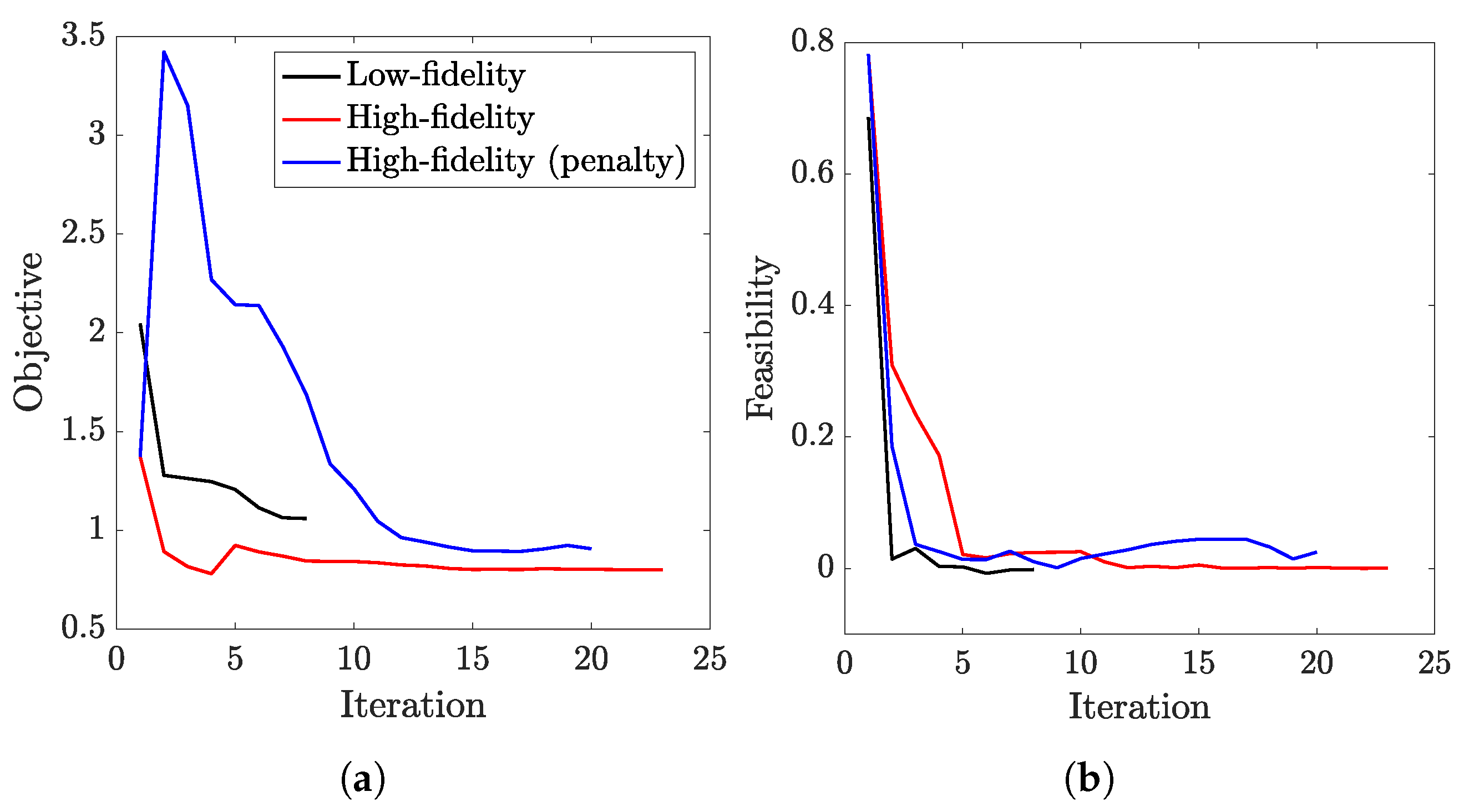
Figure 9 shows the convergence histories of the objective function and maximum constraint value. The low-fidelity run required 8 gradient calls and 23 non-gradient calls. However, the final load factor constraint was not active as expected, which could indicate issues with gradient accuracy or possibly numerical noise (which, to some extent, would also appear in the high-fidelity design space due to the regeneration of unstructured meshes). The high-fidelity run used 23 gradient calls and 62 non-gradient calls. Interestingly, the low-fidelity solution yielded a somewhat larger fuel burn (84,747 kg compared to 64,016), which more closely matches the solution reported by Brooks et al. [5] (84,072 kg). Presumably, a RANS solution would more closely match that of Brooks and the VLM method, due to the presence of viscous drag.
Because the BFGS-based optimizer considered below does not handle inequality constraints directly and thus relies on penalty constraints, the high-fidelity SLSQP case was also run using the same penalty constraint formulation, taking 20 gradient calls and 53 non-gradient calls. Unsurprisingly, the case ultimately required more iterations to converge, with the objective converging much more slowly, although the feasible design space was located more quickly. Unfortunately, the final solution found did not match that of the direct constraint handling case. This could be due to noise from remeshing or simply indicate a complex design space with local minima or very flat regions.
For reference, 
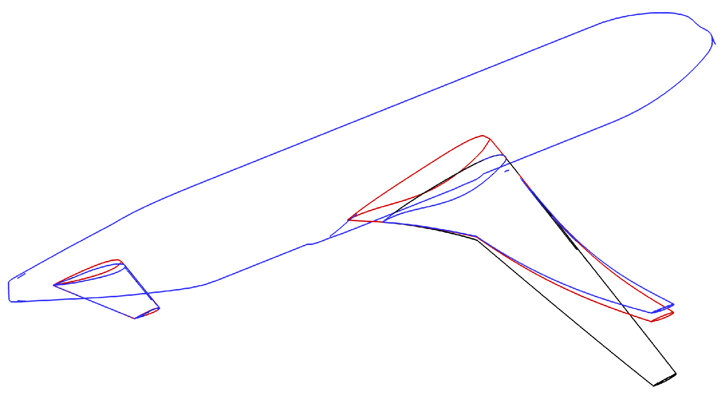
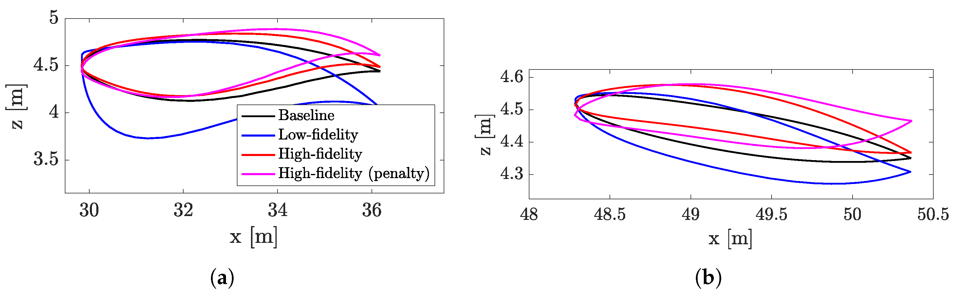
Figure 10 shows the resulting airfoil shapes at the Yehudi and tip wing sections. At the tip section, the baseline and directly constrained high-fidelity results appear to be quite similar, while larger differences can be seen in the low-fidelity and penalty-constrained high-fidelity results. While the low-fidelity result (which has higher twist and less camber) could simply be due to the lower fidelity physics (in combination with moment constraints, which would effectively influence chordwise and spanwise lift distributions), the penalty-constrained high-fidelity result (which has significantly different trailing edge camber) may be due more to numerical difficulties introduced by the penalty formulation and weights. As seen in the convergence histories, it is evident that this result followed a significantly different optimization trajectory than the directly constrained result, with the optimizer being strongly led towards a feasible design space with less emphasis on objective minimization. Traversing to the directly constrained optimum may then be difficult depending on the design space curvature; while moment constraints likely play a role in this, shock formations between the linearly interpolated Yehudi and tip sections may also be influencing lift and drag. Nonetheless, baseline and high-fidelity optimized results at the Yehudi section are fairly similar, with larger differences seen in the low-fidelity result. Here, the VLM geometry appears to be much thicker with significant differences in leading edge curvature. Unfortunately, it is unclear whether this is due more to physics or inaccuracies in shape derivatives (which has primarily been attributed to imprecise geometric sensitivities).

3.3. Airfoil Design

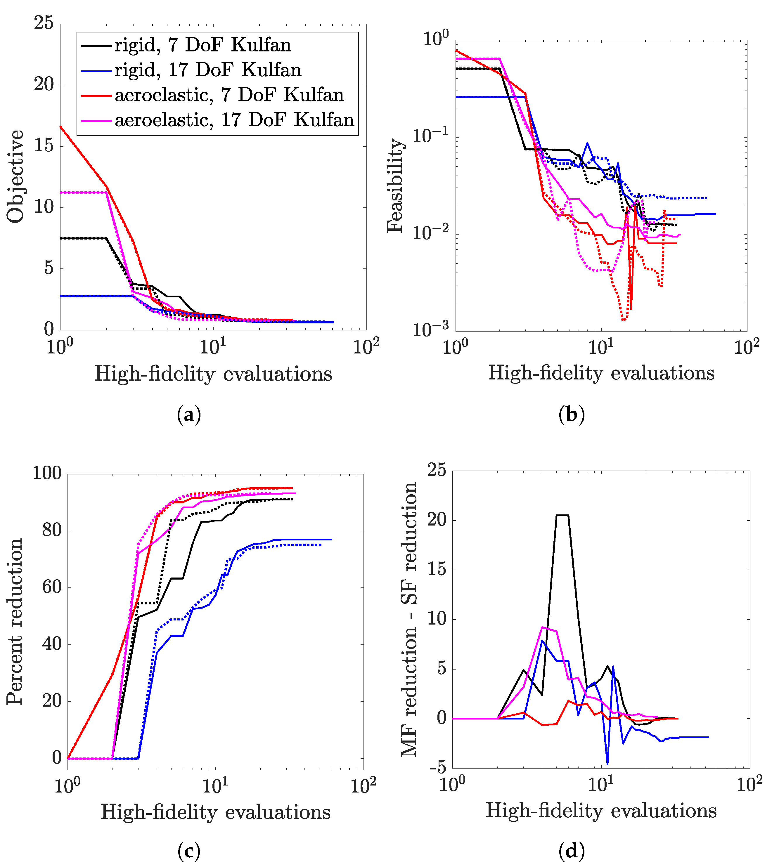
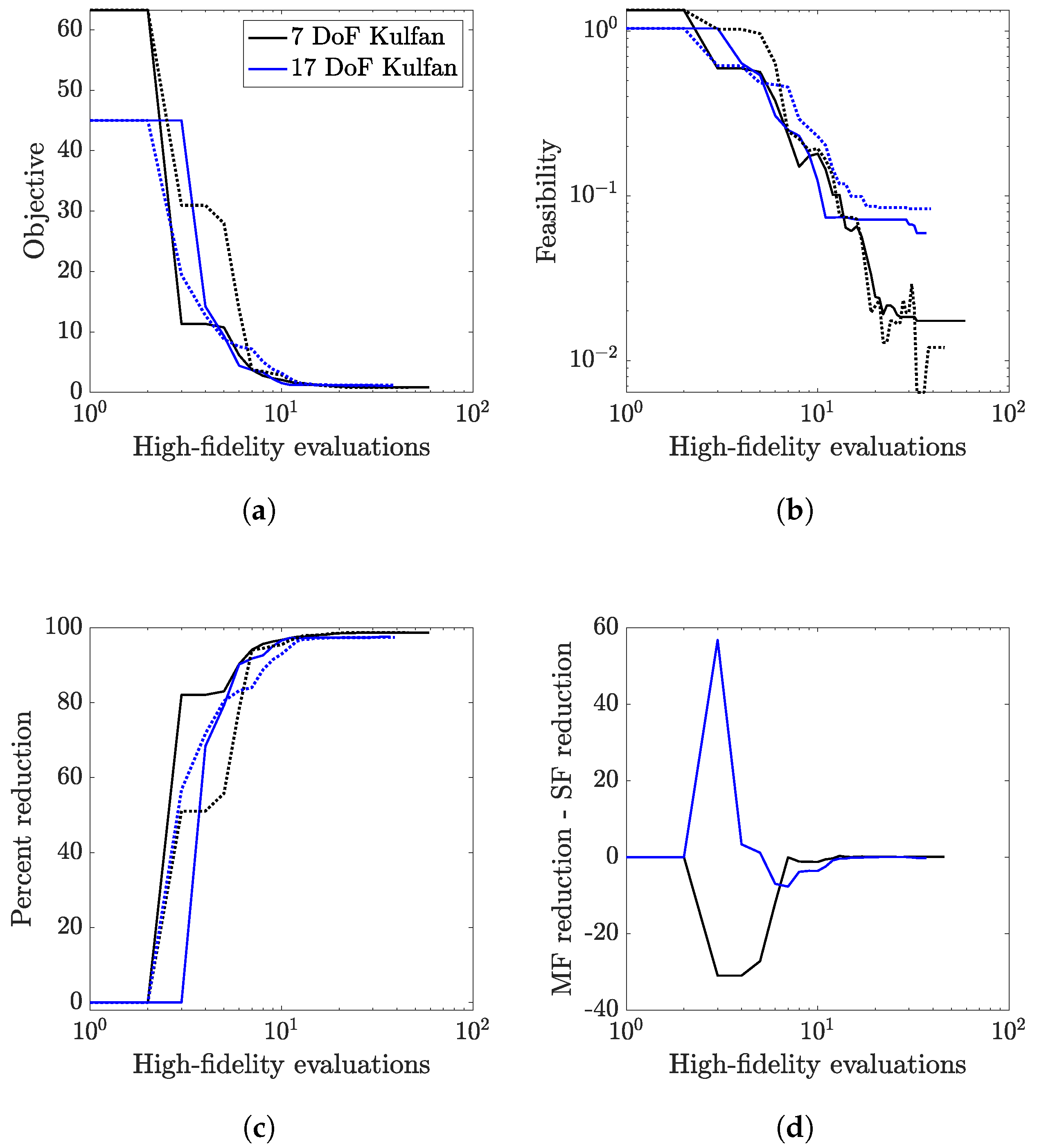
Figure 11 shows the single- and multi-fidelity convergence histories of the BFGS-based optimizers for the airfoil optimization cases (labeled problems P1a and P1b in Table 6) using rigid and aeroelastic analyses.
(The penalty-constrained, single-fidelity BFGS was selected as an algorithmically similar reference for MF-BFGS rather than SLSQP.) In particular, Figure 11a shows the penalty-constrained objective function versus the number of high-fidelity evaluations, with solid and dotted lines representing single- and multi-fidelity optimizers, respectively. This is the quantity directly minimized by the unconstrained optimizers. To illustrate how well the inequality constraints are satisfied through the penalty functions, Figure 11b shows the maximum constraint value for each case, which generally drops by roughly two orders of magnitude throughout the optimizations. Figure 11c shows the reduction in the penalty-constrained objective as a percentage of each case’s initial value. As a way to quantify the performance of using multiple fidelities, Figure 11d shows the difference of reductions (multi-fidelity minus single-fidelity). At any given design evaluation, a positive value of this metric indicates an advantage of using multiple fidelities over the single-fidelity counterpart, since it means the high-fidelity design from the multi-fidelity optimizer is better than that of the single-fidelity for the same computational cost (assuming negligible low-fidelity model cost). Note that it will approach zero if the single- and multi-fidelity optimizers both reach the same solution.
In general, all four cases (rigid and aeroelastic P1a and P1b) showed some benefits early in the optimization process (i.e., for around 3–10 high-fidelity evaluations). For example, at around five evaluations, three out of four cases were roughly 5–10% ahead of the single-fidelity optimizer. By 20 evaluations, the metric for some of the cases dipped below zero slightly, but generally approached zero (indicating both optimizers were approaching the same solution), with the exception of the higher-dimensional rigid case. Unfortunately, for this particular case, the multi-fidelity optimizer stopped at an optimum that was roughly 1.8% worse than that of the single-fidelity. It is unclear if this was due to errors in gradients, design space complexity (and constraint handling through penalty functions), or numerical noise due to the regeneration of unstructured meshes. Although this stalling could be algorithmic, it was presumed to be unlikely as the penalty-constrained SLSQP result in the previous section also appeared to reach a worse solution than SLSQP with direct constraint handling.

3.4. Structural Sizing

Figure 12 shows the same convergence metrics for the sizing-only cases (P2a and P2b in Table 6). While both black and blue cases have the same number of design variables (283 structural thicknesses with two angles of attack), they vary only by the airfoil parameterization numbers of DoF, with the 17-DoF one providing a slightly better match with the original CAD geometry. Note that while all other parameterizations include shape variables with remeshed OML and IML, this case uses the same meshes throughout, thus avoiding any numerical noise in the design space caused by different spatial discretizations. The IML meshes are also identical, with analyses varying only by the aerodynamics coupled to the structure. In Figure 12a–c, there do not seem to be major differences in either the convergence rates or final designs obtained. Figure 12d also shows mixed results, with the 17-DoF multi-fidelity case initially overtaking single-fidelity quickly, but subsequently oscillating near and approaching zero; meanwhile, the 7-DoF case hovers below zero in the beginning, but ultimately converges to zero.

3.5. Simultaneous Shape and Structural Design

Figure 13 shows the convergence metrics for problems P3a and P3b, which consider both shape and sizing design variables.
In general, the optimization trajectories were similar to those of the sizing-only cases, with both single- and multi-fidelity optimizers appearing to reach similar solutions. Figure 13a,b, however, appear to have more flat regions. This may in part be due to the added noise from remeshing the OML geometry rather than morphing the same mesh throughout the design space. Another possibility is that the neglect of structural design velocities caused larger inaccuracies in the stress constraint’s gradient when compared to aerodynamic load gradients. In terms of multi-fidelity benefits, similar metrics are observed in Figure 13d when compared to the sizing-only case. In particular, the 17-DoF case initially does much better, but soon dips below zero before converging to roughly zero. Meanwhile, the 7-DoF case initially drops below zero before converging to zero. This is perhaps unsurprising, as 285 of the design variables are the same as the previous cases, with only 16 or 36 shape variables being added. Thus, any difficulties the optimizers had in the previous design spaces (P2a and P2b) are likely to be present in the current ones.

3.6. Summary and Comparison

For reference, Table 7 lists the initial and final fuel burns and constraint values for the rigid cases (best observed design from either BFGS-based optimizer), while Table 8 lists them for the aeroelastic cases. Note that the initial designs are not trimmed and could therefore predict significantly different fuel burns when evaluated at level cruise. In particular, the trimmed rigid baseline designs yield fuel burns of 134,318 and 95,035 kg for the 7- and 17-DoF rigid cases, with the corresponding aeroelastic values being 159,717 and 84,744 kg. Among the rigid cases, the higher-dimensional airfoil parameterization yielded slightly lower initial and final fuel burn values when compared to the lower dimensional one. This is to be expected, as the baseline 17-DoF geometry yielded slightly better aerodynamic performance; among optimized geometries, it was able to more finely tune the geometry to improve performance.
The same trend was observed among aeroelastic shape-only cases. For comparison, the SLSQP P1a solution shown in Section 3.2 (via direct constraint handling) yielded a final fuel burn of 64,015.9 kg with the constraints being [ 3.6437 × 10 4 , 1.9921 × 10 2 , 7.9465 × 10 5 ]T, which equates to roughly 2% less than the BFGS optimizers. However, the penalty-constrained SLSQP, which is perhaps a fairer comparison to the BFGS-based optimizers, yielded a fuel burn of 72,519.3 kg with final constraints of [ 2.4784 × 10 2 , 1.3242 × 10 2 , 6.7584 × 10 3 ]T, an 11% difference. The same trend was observed to a greater extent for the sizing-only cases, with the higher dimensional airfoil producing a significantly lower fuel burn (although it is possible the P2a result stalled).
Among simultaneous shape and sizing cases (P3a and P3b), the same trend was unfortunately not observed. While P3a yielded a large decrease in fuel burn from P2a, the solution to P3b was in fact worse than P2b (same problem, but lacking shape design variables), as well as P3a (same problem, but with lower-dimensional airfoils). This seems to indicate either a local minimum or, perhaps more likely, simply a difficult problem for the optimizers to solve. Potentially, numerical noise from remeshing, as well as neglecting structural grid velocities (which may be important for the stress gradients) could be contributing factors. Nonetheless, all cases were at least successful in approximately satisfying the constraints and reducing fuel burn compared to the baseline geometry. Additionally, the single- and multi-fidelity all yielded roughly the same solution, with the exception of rigid P1b, where the multi-fidelity optimizer found a slightly worse solution.
For reference, 
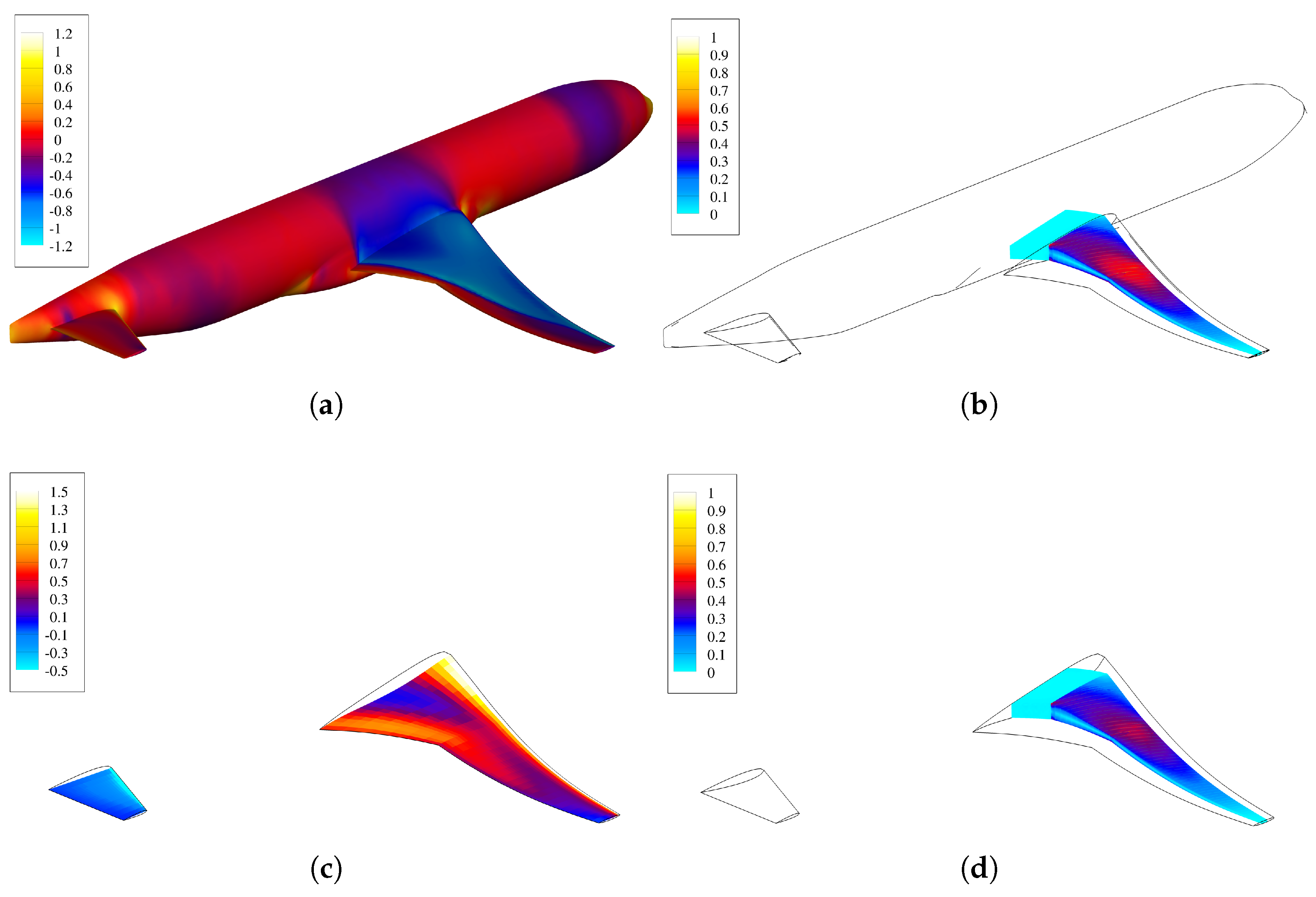
Figure 14 illustrates the baseline and optimized airfoil shapes for all cases including shape variables, where undeflected jig shapes are shown for the aeroelastic cases. In particular, the top and bottom rows show undeflected airfoil shapes at the Yehudi and tip sections, respectively. Columns from left to right show results for rigid, aeroelastic shape-only, and aeroelastic with sizing cases.
The rigid Yehudi geometries were largely unchanged, although minor shape changes were likely needed to reduce the shock strength. Rigid tip sections varied significantly in twist angle, however. This is to be expected, as aeroelastic deflection tends to cause downward wing twist, so with deflection, optimized rigid and aeroelastic geometries are likely similar in the twist angle. Visually, the aeroelastic optima with and without sizing are difficult to compare; however, both visually and in terms of final fuel burn, a higher-dimensional airfoil section (or an even higher one) appears to be necessary to obtain the “true” optimized geometry.
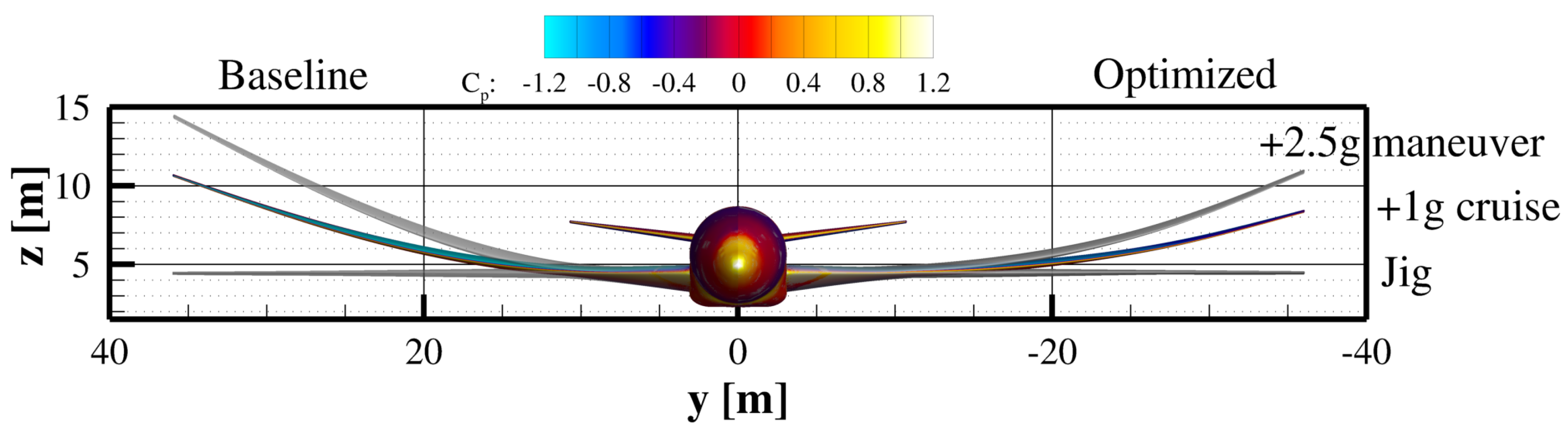
For reference, Figure 15 and Figure 16 show a sample solution to P3a, which yielded the lowest fuel burn among the shape and sizing cases. In particular, Figure 15 shows the undeflected geometry, as well as the deflected shapes during the cruise and maneuver scenarios. Shown also for reference are the trimmed baseline geometries, which had significantly larger deflections due to the lower aerodynamic efficiency, thus requiring a larger fuel mass to achieve the prescribed cruise range (and more lift to meet load factor constraints, thus leading to more induced and likely wave drag). 
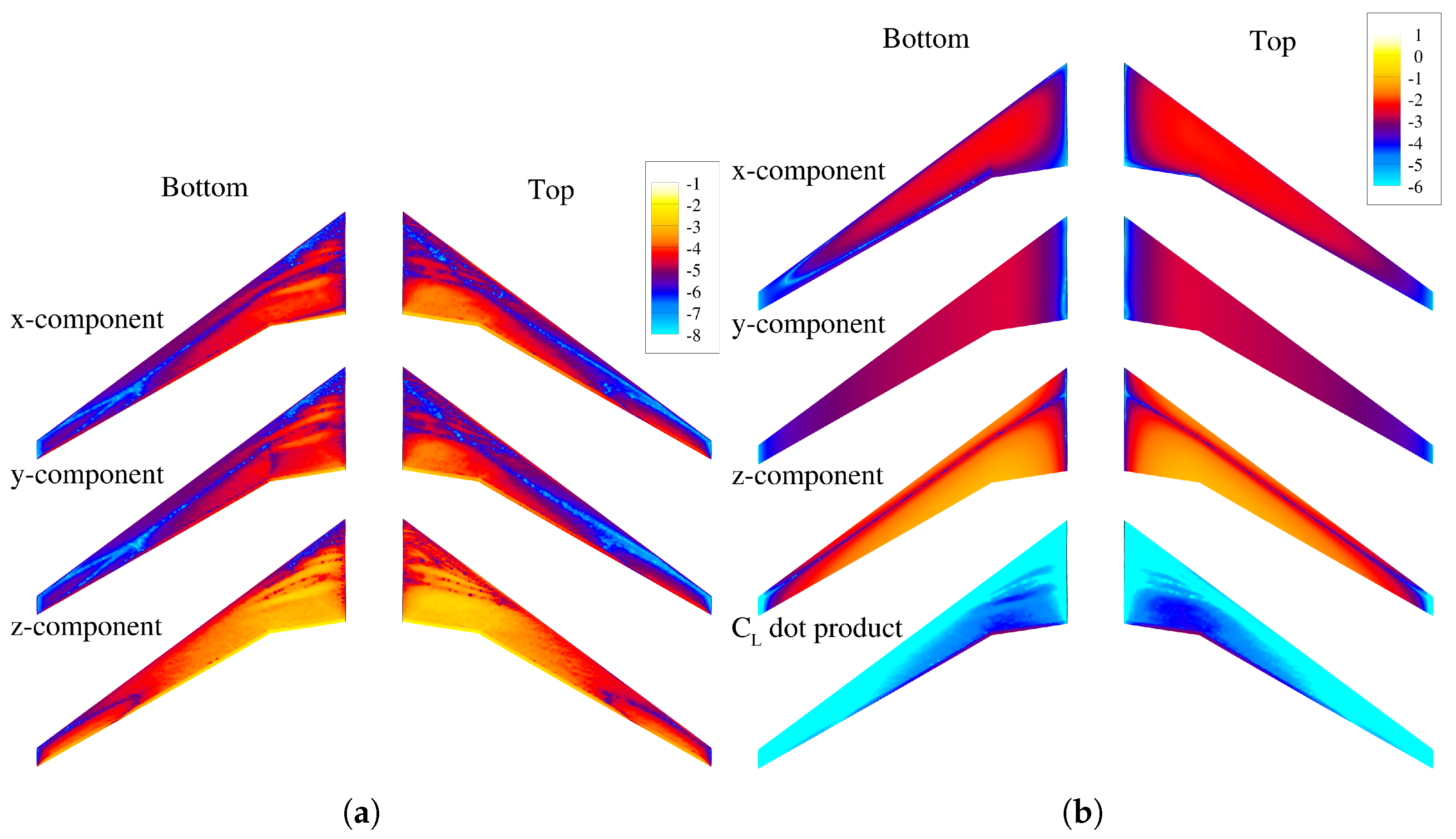
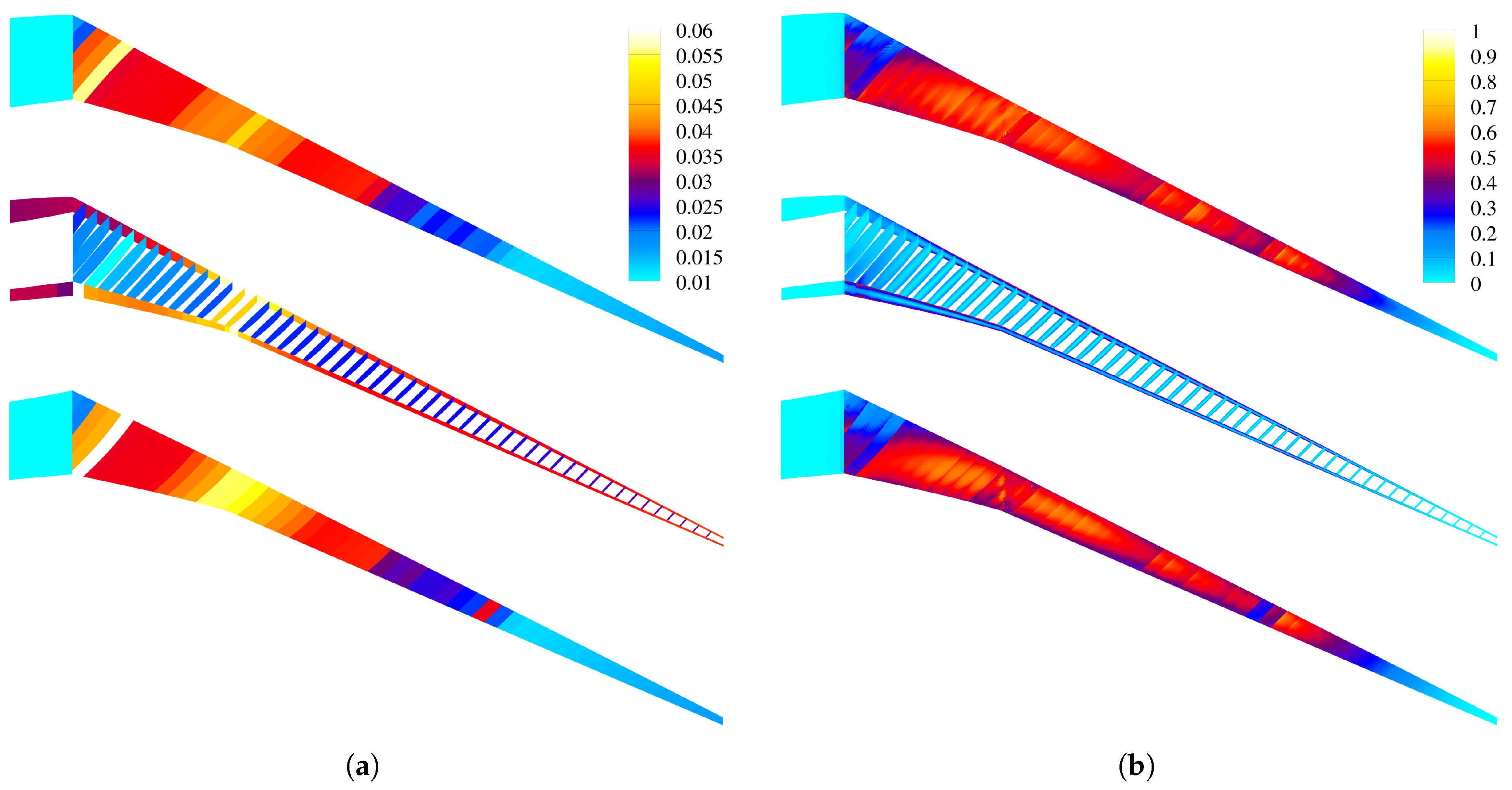
Figure 16a shows the thickness distributions of the structure, with the top, middle, and bottom showing top skins, ribs and spars, and bottom skins, respectively. Figure 16b shows the corresponding stress contours (von Mises stress normalized by yield stress) in the maneuver scenario. For reference, the stress constraint used in the optimization enforces the normalized stress to not exceed 2/3, which is the inverse of the factor of safety (1.5).
To achieve minimum structural mass while remaining feasible, the optimal stress contours would yield a maximum value of 2/3 in each structural component. This appears to be the main driver for much of the wing skins, although a handful of skins still appeared thicker than they needed to be. Elsewhere in the wing, the aerodynamic performance and trim constraints (as well as the KS aggregation) appeared to be influencing the thickness distributions as well. For instance, while the tip skin thicknesses seemed to be approaching the lower bound of 0.005 m, the tip rib and spar thicknesses remained relatively thick in spite of the low stresses in the faces. This could mean that more torsional or bending stiffness was needed to ensure an adequate lift or moment.
In general, the stress and thickness contours compared reasonably well to those of Brooks et al. [5], although the thicknesses were somewhat larger, leading to a somewhat heavier structure. Aside from optimization performance, one potential cause is the lack of stiffeners modeled in the structure, which may allow for thinner ribs and spars. The skins that intersect the wingbox trailing edge and wing–fuselage junction ribs were also quite thick and may also benefit from modeling stiffeners. There also appeared to be a stress concentration at the Yehudi on the bottom surface. This is due to the shape parameterization, as evidenced in the stress contours. Thus, more designable sections across the wing (as well as variable dihedral) may potentially prevent this.
In order to quantify the benefits of the multi-fidelity optimizer compared to its single-fidelity counterpart, 
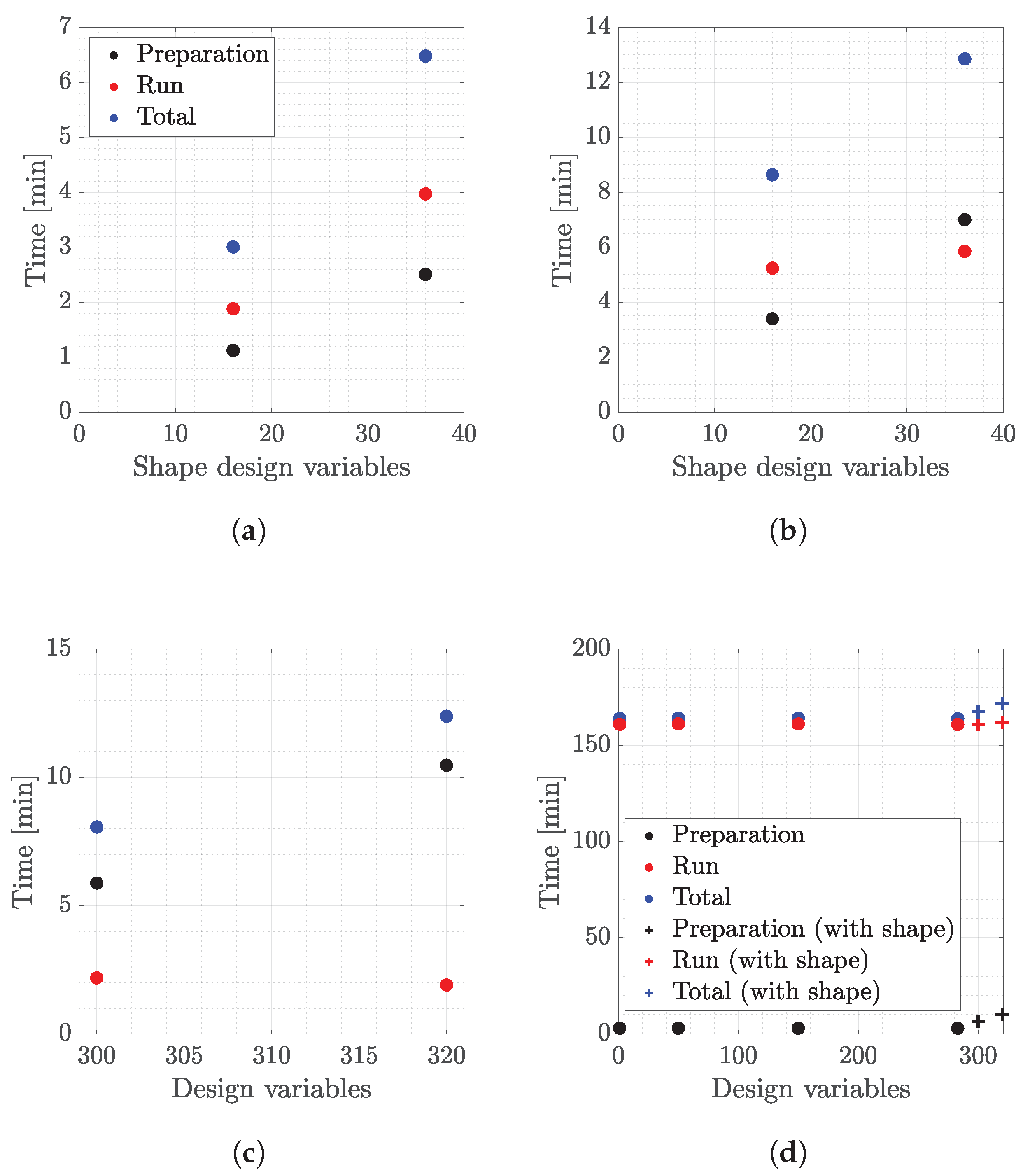
Table 9 lists the optimization costs and savings for each shape-only case. To achieve this, the best optimum from either optimizer is first identified to serve as the “true” optimum. This yields a total percent reduction in penalty-constrained objective when compared to the starting design. Specific percentages of this total reduction, ranging from 50 to 99%, are then chosen. For each optimizer, the number of high-fidelity function (and gradient) evaluations required to reach each reduction is then identified (for example, for rigid P1a, each optimizer required three function calls to achieve 50% of the total objective reduction). The cost savings associated with using the multi-fidelity optimizer compared to single-fidelity can then be computed as a percentage of the single-fidelity optimizer cost.
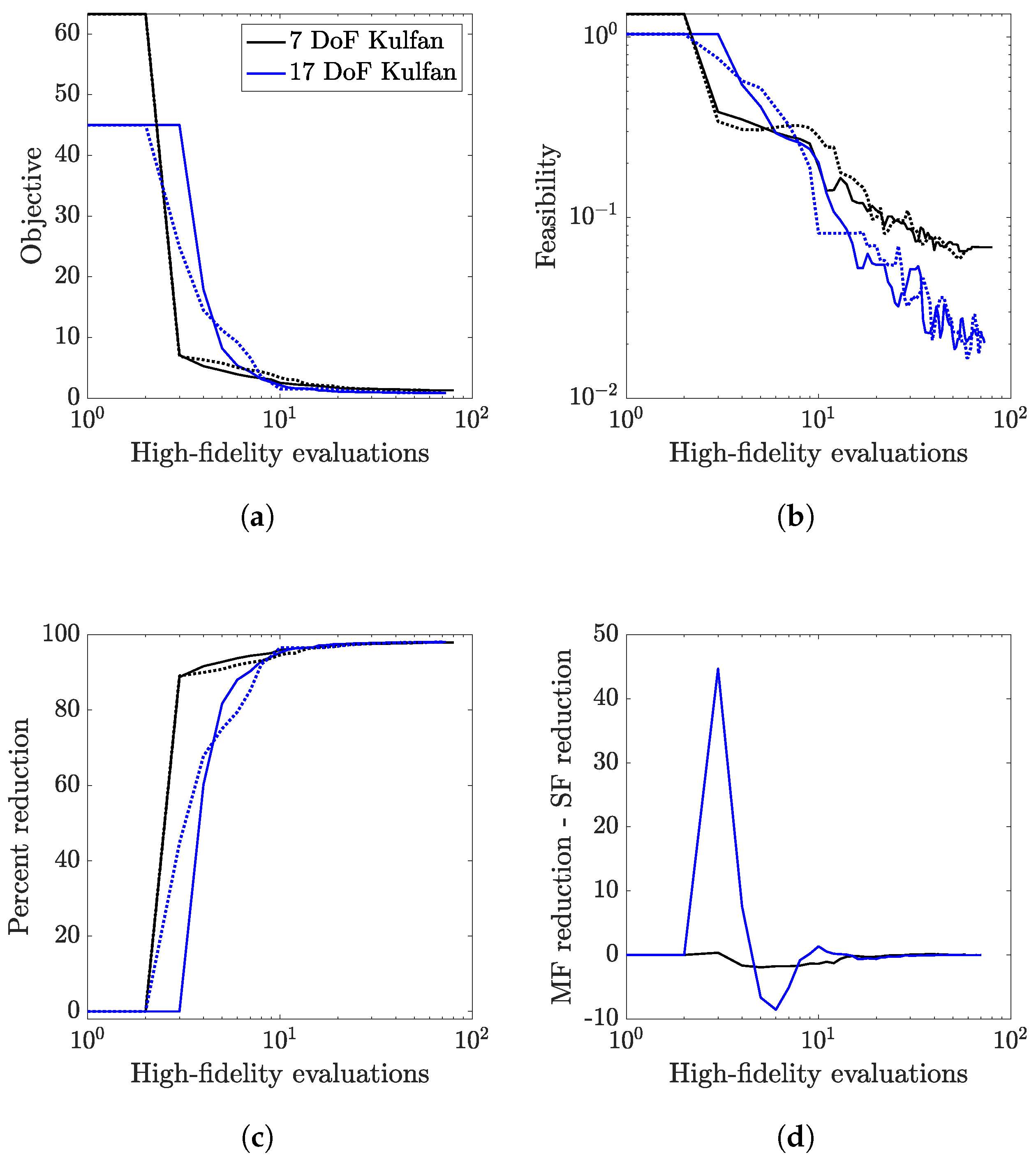
For the rigid P1a case, the multi-fidelity optimizer provided cost savings from 75 to 98% of total reduction, ranging from 20 to roughly 40%. However, by the end of the optimization, roughly where a 99% reduction was met, there were no longer any cost benefits. This is generally consistent with the metrics shown in Figure 11d, Figure 12d and Figure 13d, which suggest benefits early in the optimization process, but less as the optimization progresses. Depending on the trust region size, it may also suggest that the minimum trust region size could be increased so that the optimizer more quickly switches to high-fidelity only. The other rigid case, P1b, also showed cost savings for smaller thresholds, but was ultimately unable to achieve the 98 and 99% thresholds. Interestingly, the aeroelastic cases differed in that the savings appeared for somewhat larger thresholds. Potentially, this could mean that the different low-fidelity model is better correlated near the optimum, where shocks in the flow would be weaker.
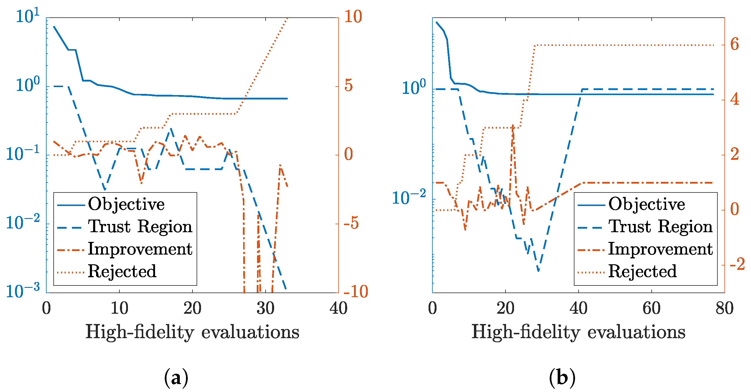
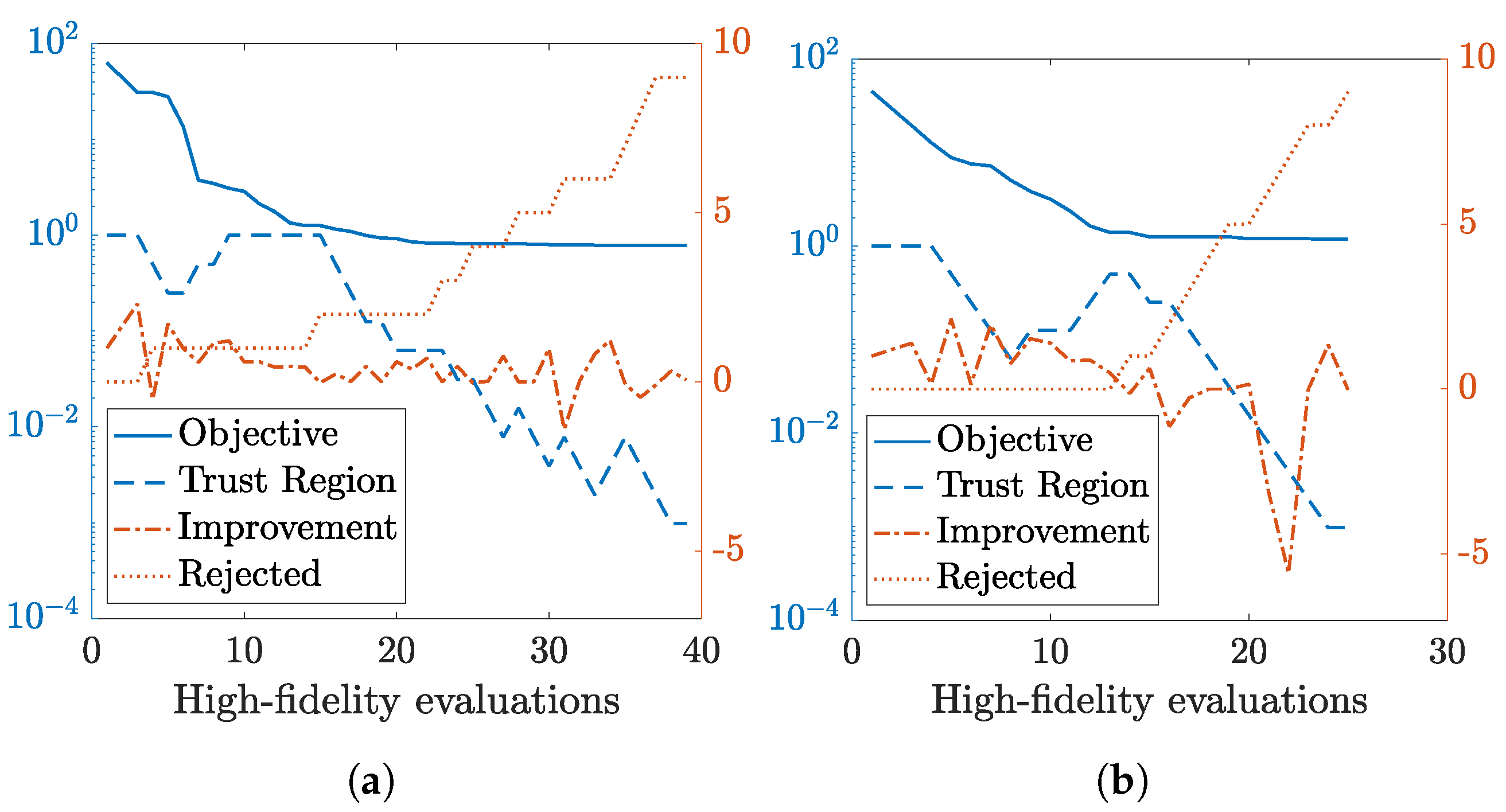
Figure 17 illustrates representative characteristics of the multi-fidelity optimization for airfoil design. Considering the comparison to the single-fidelity optimization in Figure 11 and Table 9, the multi-fidelity approach provided a cost benefit. The multi-fidelity optimizer was able to achieve most of the objective reduction within the first several high-fidelity evaluations. In the rigid P1a case (7-DoF Kulfan), after accepting the first design step, the multi-fidelity optimizer rejected the second step as the corrected low-fidelity model led to a design that increased rather than decreased the high-fidelity objective. Consequently, the trust region was halved. (The initial trust region covered the entire design domain.) The optimizer accepted the majority of subsequent steps, though the trust region steadily decreased to a size near 0.0625–0.125 (in the normalized design space D i { 0 , 1 } ). This resulted from the expected improvement ratio between the multi-fidelity and high-fidelity objectives being near enough to one to indicate that the corrected low-fidelity model was sufficient to make progress, but not accurate enough to warrant trusting over a larger space. However, after about 25 high-fidelity evaluations, the search entered a region of the design space where the multi-fidelity model was not accurate, and the optimizer rejected a series of design steps that increased the high-fidelity objective and decreased the trust region in an attempt to find a step size where the multi-fidelity model was accurate.
Of the airfoil design cases, the aeroelastic case P1a exhibited the least benefit from the multi-fidelity approach. For the first ten evaluations, the optimizer once again found the multi-fidelity model to be sufficiently accurate and maintained the trust region over the entire design domain. After that point, the multi-fidelity model did not accurately predict the high-fidelity objective, and the trust region was quickly reduced. Once the trust region had fallen below 0.001 for three consecutive iterations (a selectable parameter), the optimization reverted to single-fidelity after approximately 25 evaluations, making use of the approximate Hessian already built using high-fidelity information. Despite reverting to high-fidelity optimization, there was no discernible reduction in the objective function, suggesting that the multi-fidelity optimizer approximately found the minimum.
For reference, Table 10 lists the optimization costs for the cases with sizing. As discussed previously, the results were generally mixed, with multi-fidelity at times providing some cost savings, but often times not. Interestingly, while the cases could likely be converged more deeply, both optimizers appeared to reach a 99% reduction within 20 high-fidelity evaluations. This is likely dependent on the scale factors of the penalty functions, as the objective is generally around 0.6–2.0, with the penalty functions increasing the penalty-constrained objective by one to two orders of magnitude. Thus, much of the penalty-constrained objective reduction was achieved simply by locating a feasible design space, rather than simply reducing the fuel burn objective.
Figure 18 shows the behavior of the multi-fidelity optimizer for combined structural sizing and shape optimization. Compared to shape optimization alone (rigid and aeroelastic without sizing), the multi-fidelity optimization provided an inconsistent benefit in the 17-DoF airfoil case (P3b) and a cost penalty in the 7-DoF airfoil case (P3a). In case P3a, the multi-fidelity model had acceptable quality to maintain the trust region around 1.0 for approximately 15 evaluations, briefly reducing to 0.25. Then, the trust region was steadily reduced, though a few points were rejected due to increasing the objective function. After approximately 25 evaluations, most of the design steps were rejected and the multi-fidelity optimizer made no significant progress. While case P3b rejected fewer design steps in the first 15 evaluations, the trust region grew steadily smaller as the optimizer rejected almost all subsequent steps. Again, this was due to the expected improvement ratio being negative for both cases. With the poor agreement between high- and multi-fidelity models, the multi-fidelity optimization convergence was slow compared to single-fidelity, leading to the minimal cost benefit or penalty.

4. Discussion

The definition and implementation of a multi-fidelity, aero-structural analysis capability were described, providing the foundation for a family of benchmark problems in multi-fidelity design optimization. The models provide a rich set of selectable features, including physics coupling, data sources, parameter sets (e.g., aerodynamic shape versus structural sizing), and scalability of the design domain size. A key aspect of this work is the efficient computation of derivatives with respect to the design variables. This is a critical enabler of large-scale design optimization in both single- and multi-fidelity settings. These sensitivities were used to demonstrate gradient-based, multi-fidelity optimization for design problems that are infeasible using typical, surrogate-based multi-fidelity methods. The design domains spanned tens to hundreds of design variables, considering aerodynamic shape and structural sizing separately and in combination.
While the MF-BFGS approach was capable of performing design optimization with hundreds of variables, the scalability of the method was confounded with the consideration of different problem types. The introduction of structural sizing with hundreds of design variables required additional design constraints and gradient calculations for variables not present in the shape optimization with tens of variables. Thus, impacts on optimizer performance due to design domain dimension versus the character of the design problem could not be separated. Considering shape variables alone, MF-BFGS provides a benefit over single-fidelity BFGS in terms of objective-function reduction versus the number of high-fidelity function evaluations, whether rigid or aeroelastic. However, cases with structural sizing variables (aeroelastic only) performed less consistently. Using Kulfan airfoils with 17 degrees of freedom, the multi-fidelity optimizer produced a 45–55 percentage points greater objective function reduction than single-fidelity optimization in the first few evaluations. However, the gains were temporary, and both optimizers performed similarly in later iterations. In contrast, the seven-degree-of-freedom Kulfan cases tended to perform worse using the multi-fidelity approach in the first several iterations. This trend of the 17-degree-of-freedom airfoil exhibiting better multi-fidelity performance than the 7-degree-of-freedom airfoil was also true of the aeroelastic shape design, but not of the rigid shape design.
Several aspects could make the structural design problem more challenging than aerodynamic shape optimization. First, the sizing problem requires two additional constraints for the maneuver load factor and aggregated stress constraint. Adding these constraints to the objective as quadratic penalty terms could potentially make the design space more difficult to navigate, and the constraint penalty and KS aggregation functions require tunable parameters. The parameter selection dictates a compromise between design space curvature and constraint conservatism, which could have a significant impact on optimizer performance. Second, the aggregation of stress constraints combined with structural mesh regeneration may lead to a noisy response that slows convergence. The computation of structural shape sensitivities and the development of smoothly mapping meshes to perturbed geometry are current areas of development. Third, the external finite-differencing of the VLM mesh generation process for low-fidelity gradients and the neglect of structural design velocities (i.e., sensitivity of the structural mesh to geometry changes) could lead to inaccuracies that cause the multi-fidelity correction to suffer and produce sub-optimal line search results. Regeneration (rather than morphing) of the high-fidelity aerodynamic grids may also be a detriment due to discontinuous mesh topologies (thus causing noise in responses), although this effect would be present in the single-fidelity optimizations as well.
Finally, the variation of VLM- and Euler-CFD-based aerodynamic loads and stresses with varying structural thicknesses may simply be poorly correlated because Euler takes shocks in the flow under consideration while VLM simply uses an empirical wave drag estimate. Potentially, only a subset of the objective and constraint functions may be poorly correlated (such as the stress constraint, which was not included in the shape-only cases). How well the responses are correlated may even vary spatially, for instance agreeing well for structural groups near the tip compared to inboard (with VLM likely agreeing better when shocks are weak or nonexistent). In addition, because the VLM does have a flat-plate-based viscous drag estimate (with kinematic viscosity being set very small for the present work) and RANS flow may have weaker shocks, VLM and RANS may potentially be better correlated in spite of RANS being higher-fidelity than Euler. A subsonic cruise condition may also see better correlation between VLM and Euler or RANS.
In general, the handling of constraints is an area for improvement in gradient-based, multi-fidelity optimization. Handling constraints directly in SLSQP reduced the objective function more quickly and ultimately led to better satisfaction of the constraints compared to using a penalty function (again within SLSQP). The doubling of the objective function with penalty constraints also highlights the sensitivity of the process to weighting factors and the emphasis on constraint satisfaction versus objective improvement. The underlying BFGS method is inherently an unconstrained optimizer, and the extension of the multi-fidelity concepts to other approaches such as Sequential Quadratic Programming (SQP) is an area for future investigation.
In addition to improving the smoothness and accuracy of aeroelastic gradients, the quality of the multi-fidelity correction is an area for further investigation and future improvement. The current two-point correction is sensitive to noisy responses at either point. While first-order consistency at the current design point is necessary to prove convergence, other approaches admitting additional data could improve the correction of the low-fidelity model and be more tolerant of numerical noise. Furthermore, data-driven approaches are desired for sizing the trust region and determining when to revert to single-fidelity optimization when convergence is slow. Alternatively, adjustment of the trust region heuristic and minimum trust region size may produce improved performance.
Further expansion of the aerodynamic shape optimization may also help to demonstrate the scalability of the MF-BFGS approach. The design problem size can be expanded by increasing the airfoil degrees of freedom, as well as the number of airfoil sections. Optimization studies using Reynolds-averaged Navier–Stokes are also planned to explore performance with different fidelity combinations.

5. Conclusions

This work presented several benchmark air vehicle design problems, spanning from 10’s to 100’s of design variables, on which to test gradient-based multi-fidelity optimization algorithms. Of particular interest is the quantification of computational cost benefits associated with multi-fidelity optimizers (with this work showcasing a BFGS-based algorithm) compared to their single-fidelity counterparts. For problems focused on airfoil shape, the multi-fidelity approach consistently reduced the number of high-fidelity evaluations required relative to single-fidelity optimization, though this was not the case when considering structural sizing variables. Challenges encountered in the process, including both modeling-related (e.g., geometry and mesh construction) and optimization-related (e.g., constraint handling) were also discussed. While the multi-fidelity, gradient-based approach was successful in optimizing problems with hundreds of variables (infeasible with other typical multi-fidelity methods), it was difficult to separate the scalability of the optimizer from other process-related challenges in the optimization convergence.

Author Contributions

Conceptualization, A.S.T., D.E.B. and P.S.B.; methodology, A.S.T. and D.E.B.; software, A.S.T., D.E.B. and B.K.S.; validation, A.S.T.; formal analysis, A.S.T.; investigation, A.S.T.; resources, P.S.B.; data curation, A.S.T.; writing—original draft preparation, A.S.T., D.E.B. and P.S.B.; writing—review and editing, A.S.T., D.E.B., B.K.S. and P.S.B.; visualization, A.S.T. and D.E.B.; supervision, D.E.B. and P.S.B.; project administration, D.E.B. and P.S.B.; funding acquisition, P.S.B. All authors have read and agreed to the published version of the manuscript.

Funding

This research and the APC were funded by the US Air Force Research Laboratory (AFRL). A. Thelen and P. Beran acknowledge support of the US Air Force Office of Scientific Research (Grant 20RQCOR055, Fariba Fahroo, Computational Mathematics Program Officer). B. Stanford was supported by the Transformational Tools and Technologies project of the NASA Transformative Aeronautics Concept Program.

Institutional Review Board Statement

Not applicable.

Informed Consent Statement

Not applicable.

Data Availability Statement

Not applicable.

Acknowledgments

The authors gratefully acknowledge Kevin Jacobson (NASA Langley Research Center) for assistance in integrating with FUNtoFEM and MPHYS.

Conflicts of Interest

The authors declare no conflict of interest. The funders had no role in the design of the study; in the collection, analyses, or interpretation of the data; in the writing of the manuscript; nor in the decision to publish the results.

Abbreviations

The following abbreviations are used in this manuscript:
AIMAnalysis Interface Module
LFLow-Fidelity
HFHigh-Fidelity
SFSingle-Fidelity
MFMulti-Fidelity
MF-BFGSMulti-Fidelity Broyden–Fletcher–Shannon–Goldfarb quasi-Newton method
TRMMTrust Region Model Management
CFDComputational Fluid Dynamics
VLMVortex Lattice Method
CADComputer-Aided Design
CAPSComputational Aircraft Prototype Syntheses
IMLInner Mold Line
OMLOuter Mold Line
uCRMundeflected Common Research Model
ESPEngineering Sketch Pad
RANSReynolds-Averaged Navier–Stokes

References

  1. Jameson, A. Aerodynamic design via control theory. J. Sci. Comput. 1988, 3, 233–260. [Google Scholar] [CrossRef] [Green Version]
  2. Martins, J.R.R.A. A Coupled-Adjoint Method for High-Fidelity Aero-Structural Optimization. Ph.D. Thesis, Stanford University, Stanford, CA, USA, 2002. [Google Scholar]
  3. Martins, J.; Alonso, J.; Reuther, J. A Coupled-Adjoint Sensitivity Analysis Method for High-Fidelity Aero-Structural Design: Special Issue on Multidisciplinary Design Optimization (Guest Editor: Natalia Alexandrov). Optim. Eng. 2005, 6, 33–62. [Google Scholar] [CrossRef]
  4. Kenway, G.K.W.; Kennedy, G.J.; Martins, J.R.R.A. Scalable Parallel Approach for High-Fidelity Steady-State Aeroelastic Analysis and Adjoint Derivative Computations. AIAA J. 2014, 52, 935–951. [Google Scholar] [CrossRef] [Green Version]
  5. Brooks, T.R.; Kenway, G.K.W.; Martins, J.R.R.A. Benchmark Aerostructural Models for the Study of Transonic Aircraft Wings. AIAA J. 2018, 56, 2840–2855. [Google Scholar] [CrossRef]
  6. Alyanak, E.; Durscher, E.; Haimes, R.; Dannenhoffer, J.; Bhagat, N.; Allison, D. Multi-fidelity Geometry-centric Multi-disciplinary Analysis for Design. In Proceedings of the AIAA AVIATION 2016 Forum, Washington, DC, USA, 13–17 June 2016; American Institute of Aeronautics and Astronautics: Washington, DC, USA, 2016. [Google Scholar] [CrossRef]
  7. Haimes, R.; Dannenhoffer, J. The Engineering Sketch Pad: A Solid-Modeling, Feature-Based, Web-Enabled System for Building Parametric Geometry. In Proceedings of the 21st AIAA Computational Fluid Dynamics Conference, San Diego, CA, USA, 24–27 June 2013; American Institute of Aeronautics and Astronautics: Washington, DC, USA, 2013. [Google Scholar] [CrossRef] [Green Version]
  8. Bryson, D.E.; Haimes, R.; Dannenhoffer, J. Toward the Realization of a Highly Integrated, Multidisciplinary, Multifidelity Design Environment. In AIAA SciTech 2019 Forum; American Institute of Aeronautics and Astronautics: Washington, DC, USA, 2019. [Google Scholar] [CrossRef]
  9. Kiviaho, J.F.; Jacobson, K.; Smith, M.J.; Kennedy, G. A Robust and Flexible Coupling Framework for Aeroelastic Analysis and Optimization. In Proceedings of the 18th AIAA/ISSMO Multidisciplinary Analysis and Optimization Conference, Denver, CO, USA, 5–9 June 2017. [Google Scholar] [CrossRef]
  10. Jacobson, K.; Kiviaho, J.F.; Smith, M.J.; Kennedy, G. An Aeroelastic Coupling Framework for Time-accurate Analysis and Optimization. In Proceedings of the 2018 AIAA/ASCE/AHS/ASC Structures, Structural Dynamics, and Materials Conference, Kissimmee, FL, USA, 8–12 January 2018. [Google Scholar] [CrossRef]
  11. Jacobson, K.; Stanford, B. Flutter-constrained Optimization with the Linearized Frequency-domain Approach. In Proceedings of the AIAA SciTech 2022 Forum, San Diego, CA, USA and Virtual, 3–7 January 2022; American Institute of Aeronautics and Astronautics: Washington, DC, USA, 2022. [Google Scholar] [CrossRef]
  12. Open CASCADE Technology. Available online: http://www.opencascade.org (accessed on 11 April 2022).
  13. Bryson, D.E. A Unified, Multifidelity Quasi-Newton Optimization Method with Application to Aero-Structural Design. Ph.D. Thesis, University of Dayton, Dayton, OH, USA, 2017. [Google Scholar]
  14. Bryson, D.E.; Rumpfkeil, M.P. Multifidelity Quasi-Newton Method for Design Optimization. AIAA J. 2018, 56, 4074–4086. [Google Scholar] [CrossRef]
  15. Alexandrov, N.; Dennis, J.; Lewis, R.M.; Torczon, V. A Trust Region Framework for managing the use of approximation models in optimization. Struct. Optim. 1998, 15, 16–23. [Google Scholar] [CrossRef]
  16. Giunta, A.A.; Eldred, M.S. Implementation of a Trust Region Model Management Strategy in the DAKOTA Optimization Toolkit. In Proceedings of the 8th AIAA/USAF/NASA/ISSMO Symposium on Multidisciplinary Analysis and Optimization, Long Beach, CA, USA, 6–8 September 2000. [Google Scholar] [CrossRef] [Green Version]
  17. Gano, S.E.; Renaud, J.E.; Sanders, B. Hybrid Variable Fidelity Optimization by Using a Kriging-Based Scaling Function. AIAA J. 2005, 43, 2422–2430. [Google Scholar] [CrossRef]
  18. Beran, P.S.; Bryson, D.; Thelen, A.S.; Diez, M.; Serani, A. Comparison of Multi-Fidelity Approaches for Military Vehicle Design. In Proceedings of the AIAA AVIATION 2020 FORUM, Virtual Event, Online, 15–19 June 2020; American Institute of Aeronautics and Astronautics: Washington, DC, USA, 2020. [Google Scholar] [CrossRef]
  19. Kulfan, B.; Bussoletti, J. “Fundamental” Parametric Geometry Representations for Aircraft Component Shapes. In Proceedings of the 11th AIAA/ISSMO Multidisciplinary Analysis and Optimization Conference, Portsmouth, VA, USA, 6–8 September 2006. [Google Scholar] [CrossRef] [Green Version]
  20. Kulfan, B. A Universal Parametric Geometry Representation Method—“CST”. In Proceedings of the 45th AIAA Aerospace Sciences Meeting and Exhibit, Reno, NV, USA, 8–11 January 2007. [Google Scholar] [CrossRef] [Green Version]
  21. Jia, P.; Dannenhoffer, J. Generation of PArametric Aircraft Models from a Cloud of Points. In Proceedings of the AIAA SciTech 2016 Forum, San Diego, CA, USA, 4–8 January 2016; American Institute of Aeronautics and Astronautics: San Diego, CA, USA, 2016. [Google Scholar] [CrossRef] [Green Version]
  22. Durscher, R.J.; Reedy, D. pyCAPS: A Python Interface to the Computational Aircraft Prototype Syntheses. In Proceedings of the AIAA SciTech 2019 Forum, San Diego, CA, USA, 7–11 January 2019. [Google Scholar] [CrossRef] [Green Version]
  23. Rodden, W.; Harder, R.; Bellinger, E. Aeroelastic Addition to NASTRAN; NASA-CR-3094; NASA: Washington, DC, USA, 1979.
  24. Mason, W.H. “FRICTION”. Available online: http://www.dept.aoe.vt.edu/~mason/Mason_f/MRsoft.html (accessed on 11 April 2022).
  25. Lambe, A.B.; Martins, J.R.R.A. Extensions to the Design Structure Matrix for the Description of Multidisciplinary Design, Analysis, and Optimization Processes. Struct. Multidiscip. Optim. 2012, 46, 273–284. [Google Scholar] [CrossRef]
  26. Drela, M. AVL Overview. 2017. Available online: https://web.mit.edu/drela/Public/web/avl/ (accessed on 11 April 2022).
  27. Feuillet, R.; Marcum, D.; Alauzet, F. A closed advancing-layer method for generating curved boundary layer mesh. In Proceedings of the AIAA AVIATION 2019 Forum, Dallas, TX, USA, 17–21 June 2019; American Institute of Aeronautics and Astronautics: Dallas, TX, USA, 2019. [Google Scholar] [CrossRef]
  28. Nielsen, E.J.; Diskin, B. Discrete Adjoint-Based Design for Unsteady Turbulent Flows on Dynamic Overset Unstructured Grids. AIAA J. 2013, 51, 1355–1373. [Google Scholar] [CrossRef] [Green Version]
  29. Doyle, S.; Robinson, J.; Danials, A.; Blelloch, P.; Kalutsky, N. PyNastran: A Python-Based Interface Tool for Nastran’s File Formats. 2020. Available online: https://github.com/SteveDoyle2/pyNastran (accessed on 11 December 2020).
  30. Kennedy, G.J.; Martins, J.R. A parallel finite-element framework for large-scale gradient-based design optimization of high-performance structures. Finite Elem. Anal. Des. 2014, 87, 56–73. [Google Scholar] [CrossRef]
  31. Gur, O.; Bhatia, M.; Schetz, J.A.; Mason, W.H.; Kapania, R.K.; Mavris, D.N. Design Optimization of a Truss-Braced-Wing Transonic Transport Aircraft. J. Aircr. 2010, 47, 1907–1917. [Google Scholar] [CrossRef]
  32. Nielsen, E.J.; Park, M.A. Using an Adjoint Approach to Eliminate Mesh Sensitivities in Computational Design. AIAA J. 2006, 44, 948–953. [Google Scholar] [CrossRef] [Green Version]
  33. Gray, J.S.; Hwang, J.T.; Martins, J.R.R.A.; Moore, K.T.; Naylor, B.A. OpenMDAO: An open-source framework for multidisciplinary design, analysis, and optimization. Struct. Multidiscip. Optim. 2019, 59, 1075–1104. [Google Scholar] [CrossRef]
  34. Jacobson, K.E. Adjoint-Based Aeroelastic Optimization with High-Fidelity Time-Accurate Results. Ph.D. Thesis, Georgia Institute of Technology, Atlanta, GA, USA, 2019. [Google Scholar]
  35. Kreisselmeier, G.; Steinhauser, R. Systematic Control Design by Optimizing a Vector Performance Index. In International Federation of Active Controls Symposium on Computer Aided Design of Control Systems; Elsevier: Zurich, Switzerland, 1979. [Google Scholar]
  36. Poon, N.M.K.; Martins, J.R.R.A. An Adaptive Approach to Constraint Aggregation using Adjoint Sensitivity Analysis. Struct. Multidiscip. Optim. 2007, 34, 61–73. [Google Scholar] [CrossRef]
  37. Martins, J.; Ning, A. Engineering Design Optimization; Cambridge University Press: Cambridge, UK, 2021. [Google Scholar]
  38. Jones, D.R.; Schonlau, M.; Welch, W.J. Efficient Global Optimization of Expensive Black-Box Functions. J. Glob. Optim. 1998, 13, 455–492. [Google Scholar] [CrossRef]
  39. Zhu, C.; Byrd, R.H.; Lu, P.; Nocedal, J. Algorithm 778: L-BFGS-B: Fortran Subroutines for Large-Scale Bound-Constrained Optimization. ACM Trans. Math. Softw. 1997, 23, 550–560. [Google Scholar] [CrossRef]
  40. Morales, J.L.; Nocedal, J. Remark on Algorithm 778: L-BFGS-B: Fortran Subroutines for Large-Scale Bound Constrained Optimization. ACM Trans. Math. Softw. 2011, 38, 1–4. [Google Scholar] [CrossRef]
  41. Bryson, D.E.; Rumpfkeil, M.P. Aerostructural Design Optimization Using a Multifidelity Quasi-Newton Method. J. Aircr. 2019, 56, 2019–2031. [Google Scholar] [CrossRef]
  42. Bryson, D.E.; Rumpfkeil, M.P. All-at-once approach to multifidelity polynomial chaos expansion surrogate modeling. Aerosp. Sci. Technol. 2017, 70, 121–136. [Google Scholar] [CrossRef]
Figure 1. Baseline ESP representation of the uCRM geometry, with grey and red showing outer mold line (OML) and inner mold line (IML) geometries, respectively.
Algorithms 15 00131 g001
Figure 2. ESP parameterization of the uCRM. (a) ESP geometry used for LF analyses showing designable airfoil shapes at the wing Yehudi and tip. (b) Faces of IML geometry components with varying thickness (color variations only used to denote different components).
Algorithms 15 00131 g002
Figure 3. Extended Design Structure Matrix (XDSM) [25] depicting couplings of meshing and analysis for multi-fidelity, multidisciplinary analysis. Multidisciplinary elements are shown in green, structures in yellow, and aerodynamics in blue. Low-fidelity aerodynamics’ pre-processing is distinguished from high-fidelity using dark blue with faded inputs and outputs.
Algorithms 15 00131 g003
Figure 4. Pressure coefficient and stress (normalized by yield stress) at the same statically deflected design. The aluminum skin, rib, and spar faces have arbitrary thicknesses of 2, 3, and 4 cm, respectively. (a) Pressure coefficient, Euler. (b) Normalized von Mises stress, Euler. (c) Differential pressure coefficient, VLM. (d) Normalized von Mises stress, VLM.
Algorithms 15 00131 g004
Figure 5. Outlines of the deflected geometries, showing the Euler model’s slightly larger deflection (black: undeflected, blue: deflected Euler, red: deflected VLM).
Algorithms 15 00131 g005
Figure 6. HF adjoint, geometric sensitivities, and their dot product around the baseline aeroelastic solution. (a) Log-scale lift coefficient sensitivity. (b) Log-scale Yehudi twist sensitivity.
Algorithms 15 00131 g006
Figure 7. Mean case preparation and run times (wall-clock) as a function of shape design variables. The adjoint-based analyses (Subplots (bd)) include one forward and three adjoint solves. (a) Low-fidelity rigid; (b) High-fidelity rigid; (c) Low-fidelity aeroelastic; (d) High-fidelity aeroelastic.
Algorithms 15 00131 g007
Figure 8. Extended design structure matrix diagram of the multi-fidelity BFGS process. Blue elements represent iterative processes (i.e., optimization convergence or line searching); red represents the fidelity switching decision; green represents the calculation of values involved in the optimization process.
Algorithms 15 00131 g008
Figure 9. Convergence histories of aeroelastic problem P1a using SLSQP. (a) Objective; (b) Feasibility.
Algorithms 15 00131 g009
Figure 10. Baseline and optimized geometries. For reference, the low- and high-fidelity angles of attack are 1.339148 and 0.8001988 degrees, respectively. (a) Yehudi; (b) Tip.
Algorithms 15 00131 g010
Figure 11. Optimization results for airfoil design cases. In (ac), solid and dotted lines represent single- and multi-fidelity results, respectively. (a) Penalty-constrained objective; (b) Feasibility; (c) Percent reduction, all; (d) Percent reduction, difference.
Algorithms 15 00131 g011
Figure 12. Optimization results for structural sizing cases, fixed airfoils. (a) Penalty-constrained objective; (b) Feasibility; (c) Percent reduction, all; (d) Percent reduction, difference.
Algorithms 15 00131 g012
Figure 13. Optimization results for structural sizing cases, variable airfoils. (a) Penalty-constrained objective; (b) Feasibility; (c) Percent reduction, all; (d) Percent reduction, difference.
Algorithms 15 00131 g013
Figure 14. Baseline and optimized airfoil shapes, where aeroelastic cases show the undeflected jig shapes. (a) Yehudi, rigid; (b) Yehudi, aeroelastic; (c) Yehudi, aeroelastic with sizing; (d) Tip, rigid; (e) Tip, aeroelastic; (f) Tip, aeroelastic with sizing.
Algorithms 15 00131 g014
Figure 15. Baseline and optimized jig shapes and deflected geometries in 1g cruise and 2.5 g pull-up conditions (7-DoF airfoil parameterization).
Algorithms 15 00131 g015
Figure 16. Stress and thickness contours of the best shape+sizing optimization solution (P3a). (a) Structural thicknesses; (b) von Mises over yield stress for a +2.5 g maneuver.
Algorithms 15 00131 g016
Figure 17. Performance of multi-fidelity model within airfoil design. (a) Rigid 7-DoF Kulfan; (b) Aeroelastic 7-DoF Kulfan.
Algorithms 15 00131 g017
Figure 18. Performance of multi-fidelity model within simultaneous shape and structural design. (a) 7 DoF Kulfan; (b) 17 DoF Kulfan.
Algorithms 15 00131 g018
Table 1. Modeling fidelity by response type. (“*” denotes gradient computation through forward differencing of tool chain.)
ResponseFidelities and Solvers
Low-Fidelity (LF)High-Fidelity (HF)
RigidAVL [26] + Korn wave drag *FUN3D [28] Euler
AeroelasticVLM + TACS [30]FUN3D [28] Euler + TACS [30]
via MPHYS [11]via FUNtoFEM [9,10]
Table 2. Derivatives of the lift coefficient with respect to shape and thickness design variables. Finite difference results are forward differenced with a relative step size of 0.01 for the shape variable and 0.0001 for the structural variable.
VariableModelAdjointFinite DifferenceDifference (%)
Yehudi twistLow-fidelity aeroelastic0.040260.037966.06
High-fidelity aeroelastic0.054050.053940.203
High-fidelity rigid0.079580.079540.052
t 42 Low-fidelity aeroelastic0.064360.064310.088
High-fidelity aeroelastic0.071600.071490.157
Table 3. Fixed parameters used for the objective and constraints. Note that engine diameter and mass (based on Boeing 777-200ER/GE90) are only used in the pitching moment constraints (by means of thrust and mass).
DescriptionValueUnits
Design range7725nmi
Specific fuel consumption0.53lbm/(lbf*h)
Engine diameter2.85m
Takeoff fuel burn2.5% MTOW
Landing fuel burn1.0% Mass at end of cruise
Fixed mass91,250kg
Payload mass34,000kg
Reserve fuel mass15,000kg
Engine mass16,564kg
Structural mass for rigid cases27,250kg
Fixed mass center of gravity x-coordinate0.569Fraction of fuselage length
Payload mass center of gravity x-coordinate0.569Fraction of fuselage length
Maneuver load factor2.5g
KS stress factor of safety1.5-
Cruise Mach number0.85-
Cruise altitude37,000ft
Maneuver Mach number0.64-
Maneuver altitudeSea level-
Table 4. Penalty factors and offsets for the different inequality constraints.
DescriptionEquationsFactorOffset
Cruise load factor(21)25−0.001
Cruise moment(22) and (23)100−0.0005
Maneuver load factor(24)25−0.001
KS stress at maneuver(25)25−0.001
Table 5. Design variable designations for the different parameterizations.
ShapeStructuralAerodynamic
AirfoilTwist
Vector name x s a x s t x t x a
Dimensionality14 (7 DoF) or 34 (17 DoF)22831 or 2
Table 6. Optimization problem labels. Problems 2 and 3 are only solved with aeroelastic models rather than rigid as well, as they include structural sizing and stress constraints.
CaseDVsAirfoil DoF# DVsConstraint Equations
P1a { x s a , x s t , x a } 717(21)–(23)
P1b { x s a , x s t , x a } 1737(21)–(23)
P2a { x t , x a } 7285(21)–(25)
P2b { x t , x a } 17285(21)–(25)
P3a { x s a , x s t , x t , x a } 7301(21)–(25)
P3b { x s a , x s t , x t , x a } 17321(21)–(25)
Table 7. Summary of rigid optimization cases (subscript “0” and superscript “*” denote initial and final designs.)
ProblemFB0 (kg)FB* (kg)Initial ConstraintsFinal Constraints
P1a84,166.851,899.3 (−38.34%) 5.0709 × 10 1 8.4127 × 10 3
3.6960 × 10 2 3.2446 × 10 2
1.6960 × 10 2 1.2446 × 10 2
P1b79,272.048,874.9 (−38.35%) 2.5849 × 10 1 2.5544 × 10 3
5.4214 × 10 2 3.6096 × 10 2
3.4214 × 10 2 1.6096 × 10 2
Table 8. Summary of aeroelastic optimization cases.
ProblemFB0 (kg)FB* (kg)Initial ConstraintsFinal Constraints
P1a109,846.165,360.0 (−40.50%) 7.8224 × 10 1 1.4390 × 10 2
1.8457 × 10 2 2.0931 × 10 2
1.5429 × 10 3 9.3123 × 10 4
P1b77,726.860,008.4 (−22.80%) 6.4153 × 10 1 9.9342 × 10 3
2.0298 × 10 2 2.9444 × 10 2
2.9824 × 10 4 9.4445 × 10 3
P2a109,846.193,845.3 (−14.57%) 7.8224 × 10 1 6.8507 × 10 2
1.8457 × 10 2 1.7051 × 10 2
1.5429 × 10 3 2.9491 × 10 3
1.3408 × 10 0 6.7895 × 10 3
2.6601 × 10 1 1.6474 × 10 2
P2b77,726.867,303.7 (−13.41%) 6.4153 × 10 1 2.0281 × 10 2
2.0298 × 10 2 1.7018 × 10 2
2.9824 × 10 4 2.9823 × 10 3
1.0383 × 10 0 6.1785 × 10 4
5.2509 × 10 1 4.3878 × 10 3
P3a109,846.162,179.5 (−43.39%) 7.8224 × 10 1 1.1984 × 10 2
1.8457 × 10 2 2.3495 × 10 2
1.5429 × 10 3 3.4952 × 10 3
1.3408 × 10 0 4.6511 × 10 3
2.6601 × 10 1 4.1505 × 10 3
P3b77,726.872,152.8 (−7.17%) 6.4153 × 10 1 4.5460 × 10 2
2.0298 × 10 2 3.8832 × 10 2
2.9824 × 10 4 1.8832 × 10 2
1.0383 × 10 0 2.6112 × 10 3
5.2509 × 10 1 5.9354 × 10 2
Table 9. Cost summary for airfoil optimization cases.
CaseModelThreshold (%)Reduction (%)NF (SF)NF (MF)Savings (# Evals)Savings (% of SF)
P1aRigid50.000045.56033300.0000
75.000068.340475228.5714
90.000082.008585337.5000
95.000086.5645149535.7143
98.000089.29811512320.0000
99.000090.2093161600.0000
Aeroelastic50.000047.53033300.0000
75.000071.29544400.0000
90.000085.55455500.0000
95.000090.307576114.2857
98.000093.1593118327.2727
99.000094.1099151416.6667
P1bRigid50.000038.499254120.0000
75.000057.7489111019.0909
90.000069.2986131217.6923
95.000073.14861516−1−6.6667
98.000075.458519n/an/an/a
99.000076.228524n/an/an/a
Aeroelastic50.000046.61533300.0000
75.000069.92303300.0000
90.000083.907664233.3333
95.000088.569185337.5000
98.000091.3660116545.4545
99.000092.2983157853.3333
Table 10. Cost summary for optimization cases including structural sizing.
CaseThreshold (%)Reduction (%)NF (SF)NF (MF)Savings (# Evals)Savings (% of SF)
P2a50.000048.97753300.0000
75.000073.46623300.0000
90.000088.15943300.0000
95.000093.057268−2−33.3333
98.000095.99581014−4−40.0000
99.000096.97541820−2−11.1111
P2b50.000049.05454400.0000
75.000073.58185500.0000
90.000088.298178−1−14.2857
95.000093.20369900.0000
98.000096.14681210216.6667
99.000097.12791621−5−31.2500
P3a50.000049.38263300.0000
75.000074.073936−3−100.0000
90.000088.888767−1−16.6667
95.000093.82707700.0000
98.000096.78991112−1−9.0909
99.000097.7776141317.1429
P3b50.000048.810943125.0000
75.000073.21635500.0000
90.000087.859668−2−33.3333
95.000092.7407910−1−11.1111
98.000095.66931012−2−20.0000
99.000096.64551113−2−18.1818
Publisher’s Note: MDPI stays neutral with regard to jurisdictional claims in published maps and institutional affiliations.

