1. Introduction
Decision support systems (DSSs) are well-established types of information systems with the primary purpose of improving decision making based on data and analysis. They analyze massive amounts of data through the comprehensive compilation of information to solve problems and support decision making. With this information, the system produces reports that may project revenue, sales, or manage inventory. These systems are very important for many different industries, from healthcare to agriculture. A medical clinician using a computerized decision support system which combines the clinician inputs and previous electronic health records can assist in diagnosing and prescribing the patient.
Healthcare is one of the fastest growing sectors and is currently in the middle of a global overhaul and transformation. Global healthcare costs, currently estimated between USD 6 trillion and USD 7 trillion, are projected to reach more than USD 12 trillion in 2024 [
1]. Regarding this rapid growth in costs, measures need to be taken in order to ensure that healthcare costs do not further spin out of control. Machine learning has been identified as having major technological applications in the healthcare realm, where it will probably never completely replace physicians but will certainly transform the healthcare sector, benefiting both patients and providers.
Machine learning is a subfield of artificial intelligence that gives computers the ability to learn. It focuses on the use of data and algorithms to imitate the way in which humans learn [
2]. The process of learning starts with data observation with examples, direct experience or instruction, so it can look for patterns in the provided data to support decisions in the future. The goal is to allow computers to learn automatically without human intervention and automatically adjust actions accordingly [
3].
Machine learning algorithms are often categorized as either supervised and unsupervised. Supervised machine learning algorithms learn from labeled examples so new data can be predicted. The learning algorithm compares the output with the correct result, finding errors in order to modify the model accordingly. Unsupervised machine learning algorithms are characterized as systems that do not know the right output but explore the data and draw inferences from datasets to describe hidden structures from unlabeled data.
Clustering is considered to be the most important technique of unsupervised learning [
4]. The definition of a cluster might be seen as a collection of data objects which are similar to one another within the same group and are different from the objects in other clusters. Clustering can work as a standalone tool to derive insights about the data distribution or as a preprocessing step in other algorithms.
Most works in the industry apply supervised machine learning techniques as they are more prone to using such techniques and can be clearly compared with unsupervised learning whilst supervised learning provides more relevant results; hence, artificial applications in the industry most often use supervised learning [
5].
A recent study [
6] showed that the most frequently used algorithms for prediction were Support Vector Machine followed by Naïve Bayes. However, the Random Forest algorithm presented superior accuracy. All of them are supervised machine learning techniques [
6]. Another study [
7], for cancer diagnosis, used supervised machine learning techniques, where the Support Vector Machine achieved maximum accuracy. Another study [
8] on postpartum depression used six supervised machine learning algorithms, namely Logistic Regression, Support Vector Machine, Decision Tree, Naïve Bayes, Extreme Gradient Boosting (XGBoost) and Random Forest. As a result, the Support Vector Machine model was the best-performing model.
In this paper, we applied several machine learning techniques, both supervised and unsupervised, namely Logistic Regression, Support Vector Machine, Decision Tree, K-Nearest Neighbors (KNN), Naïve Bayes and Random Forest as supervised techniques and K-Means, Spectral Clustering, Mean Shift, Density-Based Spatial Clustering of Applications with Noise (DBSCAN) and Balanced Iterative Reducing and Clustering Using Hierarchies (BIRCH) as unsupervised clustering techniques to a diabetes and human resource datasets. We also applied unsupervised clustering algorithms such as K-Means and BIRCH for preprocessing supervised techniques, namely Logistic Regression, Decision Tree and Naïve Bayes. For the implementation of these algorithms, we used the Scikit-learn library, the free software machine learning library for the Python programming language.
Our results showed the best performance for supervised techniques against unsupervised techniques. The best-performing algorithms were Random Forest, as the supervised technique, and BIRCH and Spectral Clustering, as the unsupervised techniques. The use of clustering unsupervised techniques, such as K-Means and BIRCH, for the preprocessing of supervised techniques, namely Logistic Regression, Decision Tree and Naïve Bayes, may result in a boost of performance.
The main contributions of this paper are the following:
A succinct survey of supervised and unsupervised clustering machine learning techniques;
The presentation of the best-performing supervised and unsupervised clustering machine learning techniques applied to healthcare and human resource datasets for binary classification;
The application of unsupervised clustering algorithms for preprocessing the supervised techniques.
The rest of this paper is organized as follows.
Section 2 describes the related work on supervised and preprocessing clustering techniques and
Section 3 surveys the machine learning algorithms and techniques used in the experiments.
Section 4 presents the methodology, detailing the characteristics of the datasets and the evaluation metrics that were used for the performance assessment.
Section 5 presents the experimental evaluation and
Section 6 discusses the main findings. Finally,
Section 7 presents the main conclusions and future work.
2. Related Work
This section is divided into two parts. The first part presents related research papers on decision support systems (DSSs) using supervised techniques. The second part presents related research papers using preprocessing clustering techniques.
2.1. Supervised Techniques
Regarding DSSs using supervised techniques, in [
9], the authors presented a work that showed a compilation of machine learning algorithms used in the healthcare sector and their accuracy for different diseases. The contribution of these authors is that for a specific disease, there was a study conducted in the available literature that took the best algorithms with the top performance, and a survey which was made to allow saving research time while gathering all this information in one single paper. The best-performing algorithms for different datasets varied from Logistic Regression, Decision Tree, Support Vector Machine, Random Forest, Naïve Bayes, Artificial Neural Network and K-Nearest Neighbor. Nevertheless, the work compares supervised algorithms but for different datasets which may impact the conclusions, because the best algorithm may depend on the characteristics of the dataset, the size and its features, among other particularities.
The work in [
6] presents a study that provides a wide overview of the relative performance of different variants of supervised machine learning algorithms for disease prediction. The authors remarked that the information of the relative performance can be used to aid researchers in the selection of an appropriate supervised machine learning algorithm for their studies. It was found that the Support Vector Machine algorithm is the most frequently applied, followed by Naïve Bayes. However, the Random Forest algorithm showed a superior accuracy followed by the Support Vector Machine. The research study, in addition to comparing different supervised machine learning models, does not consider variants from each algorithm, and only a comparison between the different algorithms is made but it does not consider the hyperparameters or their tuning, which obviously has an impact on the performance results.
In [
7], the authors studied three supervised machine learning techniques for cancer diagnosis using the descriptions from breast masses. The work explored the use of averaging and voting ensembles to improve predictive performance. The study aimed to demonstrate that the principals can be readily applied to other complex tasks including natural language processing and image recognition. Maximum accuracy and the area under the curve (AUC) were achieved using the Support Vector Machine algorithm, wherein the prediction performance increased marginally when the algorithms were arranged into a voting ensemble. The authors used a dataset which has a low number of instances and features which show a lack of sparsity and high dimensionality, which are computationally less demanding, but in another way, could lead to overfitting and do not generalize to other test instances.
The work in [
10] presents a case study related to mechanical ventilation, a life-saving intervention which, when improperly delivered, can affect and injure the patient. The decision support system presented promises to reduce risks by performing the per-breath classification of five of the most widely used ventilation modes in the United States of America using the high-performance supervised machine learning model Random Forest, while having to restrict the size of the training set and maintain model generalization. The authors used almost the same size training and test datasets, which normally is not recommended for creating a machine learning model. Additionally, as the ventilation modes are so heterogeneous and can be difficult to identify, the dataset classification used for training was captured by two clinicians by mere visualization, which can be erroneous in its labeling. To conclude, the gathering of data was also confined to a single academic medical center and single ventilator type, which can be a limitation for a robust and reliable machine learning model.
In [
11], the authors presented a case study of people experiencing low back pain evolving into a chronic condition, unless the patient receives the right interventions at the right moment. The research was initiated with the design of the decision support system using supervised machine learning with three classification models: Decision Tree, Random Forest and Boosted Tree. This study showed promising results with the Boosted Tree model and Decision Tree but must still be improved with the new collection of cases, classified as self-care cases. One limitation of this study was that the cases in the training dataset were fictitious cases on lower back pain collected during a vignette study with primary healthcare professionals which can impact the performance of the model. Additionally, we considered that the test dataset was excessively small, with only 38 real-life cases.
The work in [
12] presented a case study for the diagnosis of periodontal disease, which is a common infectious disease in humans that may cause cardiovascular disease and complications of coronary heart disease. With the high prevalence of periodontal disease, the prevention, identification and early treatment of periodontal disease have become extremely important. This study, using the records of 300 patients, was performed using the Support Vector Machine supervised algorithm and based on different kernel functions using the cross-validation method, showing that the radial kernel function has the best performance. Other similar studies regarding the same disease were conducted. For example, one study of 150 periodontal patients showed that the Support Vector Machine and Decision Tree have higher accuracy, while the Artificial Neural Network presented the worst results. Another study of 30 patients described the use of the Artificial Neural Network with a top precision rating. One constraint of this study was that a limited dataset size was used, where more accurate results can be obtained if more data can be used.
In [
13], the authors presented a case study of coronavirus disease 2019 (COVID-19), the acute respiratory disease that has been classified as a pandemic by the World Health Organization. It is crucial to identify the key factors for mortality prediction to optimize the patient treatment strategy. The dataset, after preprocessing, consisted of 1766 datapoints corresponding to 370 patients suspected of having COVID-19 from a Hospital in Wuhan. The study proposed supervised machine learning methods, namely Neural Networks, Logistic Regression, XGBoost, Random Forest, Support Vector Machine and Decision Tree, based on blood tests to predict COVID-19, using a strong combination of five features. The results showed that for feature importance and classification, XGBoost and Neural Network, respectively, demonstrated the top performances. Other machine learning models involving trees and regression algorithms performed the next best performance results.
The work in [
14] presented a study to support clinicians and researchers in machine learning approaches in the field of infection management. Supervised machine learning techniques were used, including Logistic Regression in 18 studies, followed by Random Forest, Support Vector Machine and Artificial Neural Networks in 18, 12 and 7 studies, respectively. The best-performing techniques were Long Short-Term Memory Networks, Artificial Neural Network, Logistic Regression, Support Vector Machine, Regression Tree and Stochastic Gradient Boosting. Some limitations of this study included the fact that the comparability of the different approaches per research area was limited and should be interpreted with great caution. There is large heterogeneity between the identified studies, namely in terms of predicted outcomes, the features used and the study size. Knowing that the operations of cleaning and transforming, normally represents the majority percentage of the entire work of applying a machine learning model to data, in 39% of the previous carried studies there was no mention to this kind of operations.
In [
8], the authors presented a study of postpartum depression, which is a depressive episode that begins within one year from childbirth, interfering with the mother’s emotional well-being but also associated with infant morbidity and poorer cognitive and behavioral skills in children later in life. Electronic health records were obtained from two Hospitals between 2015–2017 with 9980 episodes of pregnancy identified. Six supervised machine learning algorithms were used, including Logistic Regression, Support Vector Machine, Decision Tree, Naïve Bayes, XGBoost and Random Forest. The Support Vector Machine model was the best-performing model. Nevertheless, the use of multiple features from the dataset can lead to a complex system wherein the most correlated features should be chosen among the total set. Additionally, the method used for oversampling to handle an imbalanced dataset may contribute to overfitting and impacting the model performance.
The work in [
15] presented a study of the early prediction of asthma exacerbations, which is the most common and costly chronic disease in United States. For the detection of this disease, a prediction model was built using the Bayesian Classifier, Adaptative Bayesian Network and Support Vector Machine supervised algorithms. The dataset consisted of 7001 records collected using a previously prescribed remote management from home method, wherein patients used a laptop computer at home to fill in their asthma diary on a daily basis. It was found that the dataset distribution is highly skewed, where the problem was addressed by rearranging the dataset for three experiments: the first one with all the data used for training and testing; the second one with stratified samples for both training and testing; and the last one with a stratified sample for training all the remaining data for testing. Then, the three predictive models were used, wherein predictive models were trained on stratified samples, which yielded better results. Nevertheless, this study has some limitations, namely the relatively small data sample, containing limited numbers of cases of asthma exacerbations.
2.2. Preprocessing Clustering Techniques
Regarding research papers using preprocessing clustering techniques, the authors in [
16] proposed an evaluation method while using unsupervised clustering algorithms by measuring the usefulness of the task under consideration. For that, they used two example scenarios, among which one included the use of clustering as an automated pre-processing step in a whole data-processing chain. The purpose of this was to improve the overall performance of the system, which can be quantified by some problem-dependent score. The clustering algorithm was just one more “parameter” that has to be tuned and this tuning can be achieved in the same way as for all other parameters. What matters is not the evaluation of the quality of the clustering and which meaningful groups it discovers, but the usefulness of the clustering for achieving the final goal.
The work in [
17] presented a study using stochastic gradient Markov Chain Monte Carlo (SG-MCMC) and proposed a subsampling strategy to reduce the variance of applying naïve subsampling. For that, the authors partitioned the dataset with the K-Means Clustering algorithm in a preprocessing step and used fixed clustering throughout the entire MCMC simulation. In particular, the clustering procedure was performed on the data samples only once before simulation, and during the sampling procedure, it was easier to compute the new gradient estimator without having extra overhead.
In [
18], the authors presented a study of an unsupervised clustering approach to resolve the frequent data imbalance problem in supervised learning problems in functional genomics. The study proposed preprocessing majority instances by partitioning them into clusters using class purity maximization clustering, which greatly reduced the ambiguity between minority instances and the instances in each cluster. For a moderately or highly imbalanced ratio and low in-class complexity, this technique has a better prediction accuracy than the under sampling method. For an extremely unbalanced ratio, this technique demonstrates an almost perfect recall that reduces the amount of imbalance with significant improvements over previous predictors.
The work in [
19] presents a study on hydrological models wherein the dynamic characteristics, such as seasonal dynamics, are revealed to be a model structural deficiency. The authors proposed a clustering preprocessing framework for the calibration of hydrological models to simulate seasonal dynamic behaviors. Two clustering operations were performed based on the preprocessed climatic index and land-surface index systems. The obtained results show that the performance of the model with a clustering preprocessing framework in the middle and low-flow conditions is significantly improved without reducing the simulation accuracy for high flows.
From previous research papers, the application of the clustering preprocessing technique is used for subsampling, data imbalance, or model calibration. The specific application to supervised algorithms is still uncommon to the best of our knowledge. This work intends to highlight the importance of these unsupervised techniques. Mainly, the use of clustering for preprocessing supervised algorithms may translate into a boost in their performance.
3. Machine Learning Algorithms and Techniques
In this section, we survey the algorithms and techniques used for the diabetes and human resource datasets. A brief conceptual explanation of both supervised and clustering unsupervised techniques is presented.
3.1. Logistic Regression
Logistic Regression is a supervised algorithm that is often used for predictive analytics and modeling to understand the relationship between a dependent variable and one or more independent variables, wherein probabilities are estimated using a logistic regression equation [
20]. The dependent variable is finite or categorical, whereas for binary regression, we have A or B options, and for multinomial regression, we have a range of finite options, for example A, B, C or D. Examples that use this technique can be found in [
8,
9,
13,
14].
3.2. Support Vector Machine
Support Vector Machine is a supervised algorithm whose the purpose is to find a hyperplane in an N-dimensional space with N as the number of features which distinctly classifies the data points [
21]. There are many possible hyperplanes that can separate the two classes of data points, however, we want to maximize the distance between the data points of the classes while having a plane that has a maximum margin. With this, future data points can be classified with more confidence. Among related works, [
6,
7,
8,
9,
13,
14,
15] are examples that use this technique.
3.3. Decision Tree
Decision Tree is a supervised algorithm to categorize or make predictions on how a previous set of questions were answered [
22]. As the name says, it resembles a tree wherein the base of the tree is the root node, from which we obtain a series of decision nodes that depict the decisions to be made. From the decision nodes representing the question or split point, we have leaf nodes which represent the consequences of those decisions or the answers. Examples that use this technique can be found in [
8,
9,
11,
12,
13].
3.4. Naïve Bayes
Naïve Bayes is a supervised algorithm based on the Bayes theorem as in Equation (1), where we can find the probability of
A happening, given that
B has occurred [
23].
The assumption made is that the predictors or features are independent, meaning that the presence of one particular feature does not affect the other. Even if there is dependency, all these features still independently contribute to the probability; hence, it is called naïve. Among related works, [
6,
8,
9] are examples that use this technique.
3.5. Random Forest
Random Forest is a supervised algorithm which combines the output of multiple decision trees to reach a single result [
24]. It generates a random subset of features, which ensures low correlation among decision trees. This is a key difference between decision trees and random forest. While decision trees consider all possible features splits, random forest only select a subset of those features. Examples that use this technique can be found in [
6,
8,
9,
10,
11,
13,
14].
3.6. K-Nearest Neighbors (KNN)
KNN is a supervised algorithm which estimates the likelihood that a data point will become a member of one group or another based on what group the data points nearest to it belong to [
25]. It is called a lazy learning algorithm because it does not perform any training when we supply the training data, but simply stores them during the training time and no calculations are made. KNN tries to determine what group a data point belongs to by looking at the data points around it. In related work, [
9] is an example that uses this technique.
The algorithm performs a voting mechanism to determine the class of an unseen observation where the class with the majority vote will become the class of the data point. If the value of K is equal to one, then it will use only the nearest neighbor to determine the class, and if the value of K is equal to ten, it will use the ten nearest neighbors.
3.7. K-Means
K-Means is a clustering unsupervised algorithm where the purpose is to group similar data points together and discover underlying patterns whilst looking for a fixed number (k) of clusters in the dataset [
26]. A cluster is nothing more than a collection of data points aggregated together because of certain similarities. We started to define a target number k which is the number of centroids. A centroid is the imaginary or real location representing the center of the cluster, and every data point is allocated to each of the clusters by reducing the in-cluster sum of squares. In other words, it tries to keep the centroids as small as possible. An example from the related work that uses this technique can be found in [
17].
3.8. Spectral Clustering
Spectral Clustering is a clustering unsupervised algorithm which reduces complex multidimensional datasets into clusters of similar data in rarer dimensions [
27]. It makes no assumptions about the form of the clusters. In contrast to the K-Means technique, which assumes that the points assigned to a cluster are spherical about the cluster center, Spectral Clustering helps to create more accurate clusters and can correctly cluster observations that actually belong to the same cluster. However, these are farther off than observations in other clusters due to the dimension reduction.
3.9. Mean Shift
Mean Shift is a clustering unsupervised algorithm whose purpose is to discover blobs in a smooth density of samples [
28]. It is a centroid-based algorithm that works by updating candidates for centroids to be the mean of the points within a given region, also called bandwidth. These candidates are then filtered in a post-processing stage to eliminate near-duplicates to form the final set of centroids. In contrast to K-Means, there is no need to choose the number of clusters.
3.10. DBSCAN
DBSCAN is a clustering unsupervised algorithm that groups together data points that are close to each other based on a distance measurement and a minimum number of points [
29]. It also marks the data points that are in low-density regions as outliers. Basically, this requires two parameters: the first one specifies how close data points should be to each other to be considered part of the cluster; and the second parameter is to define the minimum number of data points to form a dense region.
3.11. BIRCH
BIRCH is a clustering unsupervised algorithm that uses hierarchical methods to cluster and reduce data [
30]. The algorithm only needs to scan the dataset in a single pass to perform clustering and uses a tree structure to create a cluster which is generally called the Clustering Feature Tree. Each node of the tree is composed of several clustering features.
BIRCH is often used to complement other clustering algorithms by creating a summary of the dataset that the other clustering algorithm can now use [
31]. It can only process the metric attributes represented in Euclidean space, i.e., no categorical attributes should be present. Categorical refers to attributes that generally take a limited number of possible values that do not necessarily need to be numerical but can be textual in nature.
4. Materials and Methods
This section aims to provide the methodology, specifying the characteristics of the datasets, the applied preprocessing steps and the evaluation metrics that were used for the performance assessment.
4.1. Dataset and Preprocessing
We describe the diabetes and human resource datasets along with the preprocessing operations before submitting to the algorithms. Note that the unsupervised clustering algorithms applied for preprocessing the supervised algorithms were executed after the following preprocessing operations for the datasets.
4.1.1. Diabetes Dataset
The type II diabetes disease dataset was originally from the National Institute of Diabetes and Digestive and Kidney Diseases, and was obtained from [
32]. In particular, all the data refer to female patients that were at least 21 years old and of Pima heritage, which are Native Americans who traditionally lived along the Gila and Salt rivers in Arizona in the United States of America [
33].
The dataset has 768 records, each one of which are for a single person with eight features and a target label. The first feature, pregnancies, is the number of times that the person was pregnant. The second feature, glucose, is the plasma glucose concentration in their blood and the main indicator of diabetes. Diabetes is characterized by the difficulty or inability of the pancreas to produce insulin, a hormone that transforms glucose from food. The third feature, blood pressure, measured in units of millimeters of mercury (mmHg), is the pressure in which blood circulates within the arteries which varies throughout the day along normal values. The fourth feature, skin thickness, measured in mm, is primarily determined by collagen content and is increased when having diabetes. The fifth feature, insulin, measured in µIU/mL, is a hormone responsible for lowering blood glucose by promoting the entry of glucose into cells. The sixth feature, body mass index (BMI), measured in kg/m
2, is used to know whether the weight matches the person’s height, namely if the person is underweight, normal weight or above what would be expected for their weight. The seventh feature, diabetes pedigree function, is a function that determines the risk of type II diabetes based on family history. A bigger function indicates a greater risk of type II diabetes. The eighth feature, age, is the age of the person. The outcome target label is our target or class attribute, which is one or zero depending on whether the person has been diagnosed with type II diabetes or not, respectively. The dataset contains 268 records of persons with diabetes type II and 500 records of persons who do not, as shown in
Figure 1.
The eight features of the dataset are of numeric type, among which the BMI and diabetes pedigree function are of float type whilst all the others are of integer type. The dataset does not have any duplicate values or null values, but values of zero on features such as skin thickness, blood pressure, glucose, insulin and BMI might be considered as missing values, because that value is not reasonable or valid.
Figure 2 and
Figure 3 represent the histogram graphs for the previous features, wherein the zero value is present and considered not valid or a missing value.
To address the missing values problem, at least two different approaches can be used: the deletion of the instance or the imputation of a value. As the dataset only has 768 records, the first approach would reduce the dataset even further, which is not desirable. The second approach seems to be the most appropriate where the mean or the median can be used. The disadvantage of using the mean is that it is biased by the values at the far end of distribution, whereas in this case, the use of median is preferable, because it is a better representation of the majority of the values in the feature.
Figure 4 and
Figure 5 show the box plots for the glucose, blood pressure, skin thickness, BMI and insulin features, where the representation of outliers is present.
For the box plot of the glucose and skin thickness features, there is one outlier, where zeros have been replaced with the mean value. Blood pressure does not have many outliers, hence zeros have been replaced with the mean value. On the other hand, BMI and insulin have a large number of outliers; therefore, zeros have been replaced with the median for more accurate results.
Figure 6 shows the description of the dataset, where different scales, between minimum and maximum values, exist for the features.
Usually, machine learning algorithms present some performance problems when the input numerical attributes have different scales [
34]. In order to address this problem, min–max scaling can be used to rescale values to an interval of [0, 1]. For the diabetes disease dataset, the min–max scaling was applied to the pregnancies, glucose, blood pressure, skin thickness, insulin, BMI, diabetes pedigree function and age features.
4.1.2. Human Resource Dataset
The human resource dataset was obtained from [
35] and refers to a company’s data analytics for employee retention.
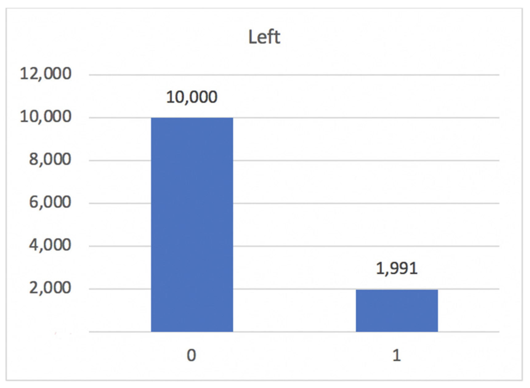
The dataset has 14,999 records, each one of which is for a single person and has nine features and a target label. The first feature, satisfaction level, is the level of satisfaction of an employee regarding their job. The second feature, last evaluation, is the rating between 0 and 1 received by an employee at his last evaluation. The third feature, number project, is the number of projects that an employee is involved in. The fourth feature, average monthly hours, is the average number of hours in a month spent by an employee at the office. The fifth feature, time spend company, is the number of years that an employee has spent in the company. The sixth feature, work accident, is a binary value where zero means that the employee had no accident during their stay and one means that the employee had accident during their stay. The seventh feature, promotion last 5 years, is the number of promotions during an employee’s stay. The eighth feature, department, is the department that an employee belongs to. The ninth feature, salary, is the level of salary an employee has, namely low, medium or high. The target label, left, is a binary value, wherein zero indicates that the employee remains in the company and one indicates that the employee left the company.
The dataset does not contain missing or null values but contains duplicate records. The duplicates were eliminated, resulting in 10,000 records of employees remaining in the company and 1991 records of employees leaving, as shown in
Figure 7.
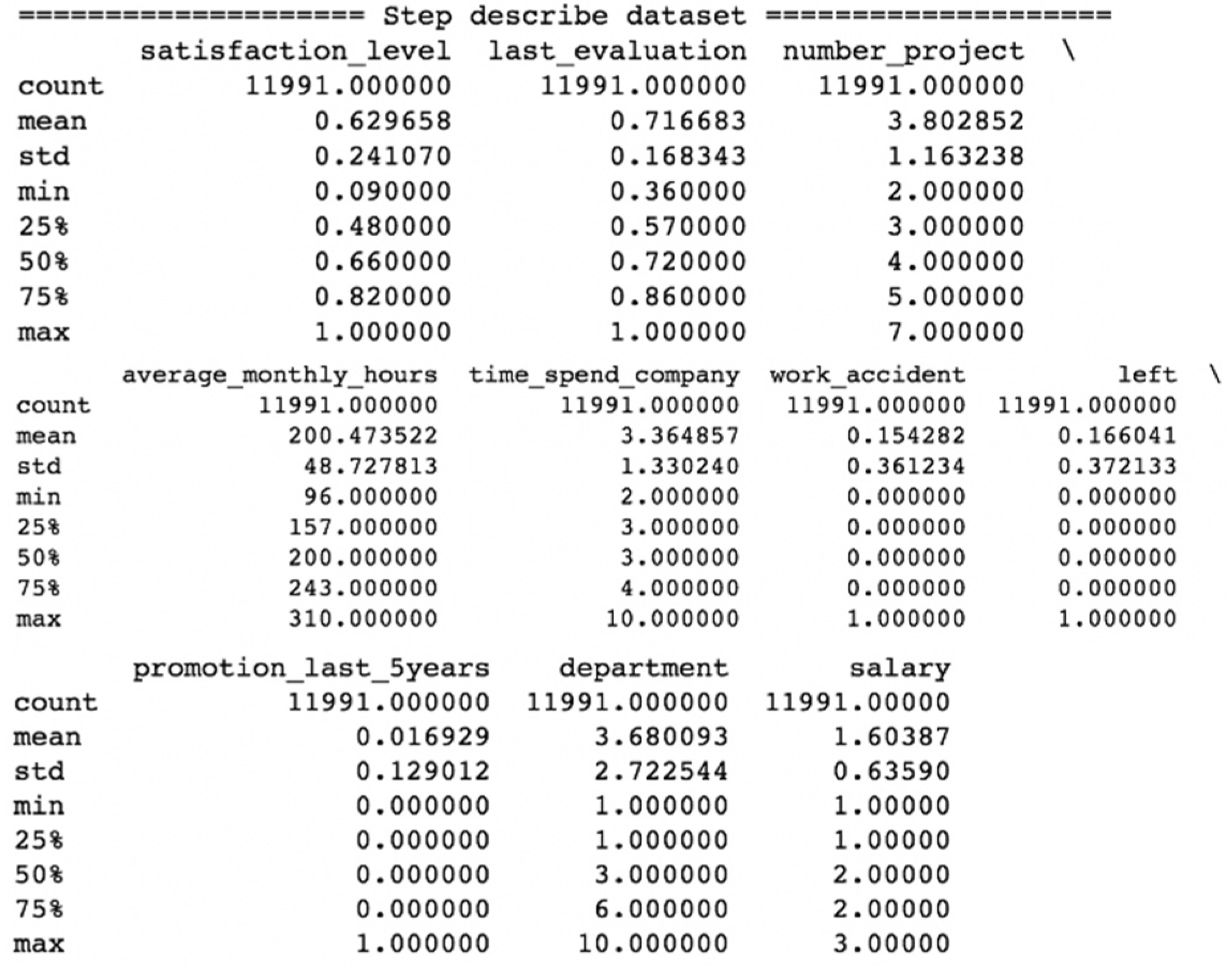
The features satisfaction level and last evaluation of the dataset are of float continuous numeric type. The features number project, average monthly hours and time spend company are of integer numeric type, while the features work accident and promotion last are of categorical numeric type and the department of the categorical type. The last feature salary is of ordinal type.
In order to have inputs as numeric type for the algorithms, a conversion to numeric was made for the feature department and salary.
Figure 8 shows the description of the dataset, wherein only the feature average monthly hours has a different scale from the remaining feature, and min–max scaling was applied to this feature.
4.2. Feature Selection
Before starting the process of feature selection, we created new features from the available variables. The main goal was to create new features that might be more useful to the prediction process where these new features are always created based on current data. Less correlation with the target labels outcome and left means values near zero and stronger correlations with values near 1 or −1.
After combining the features, we implemented feature selection to reduce the number of input features when developing a predictive model because high dimensional data contain features that are irrelevant or redundant for the algorithm’s performance. For that, we used ANOVA, which is an acronym for analysis of variance and is a parametric statistical hypothesis test for determining whether the means from two or more samples of data come from the same distribution [
36]. It can be used for feature selection when we have numerical input data and a categorical target variable. This model does not consider which classifier is going to be used but focuses on the relationship between features and the target, which is the variable whose values are to be modeled and predicted by other variables.
4.2.1. Diabetes Dataset
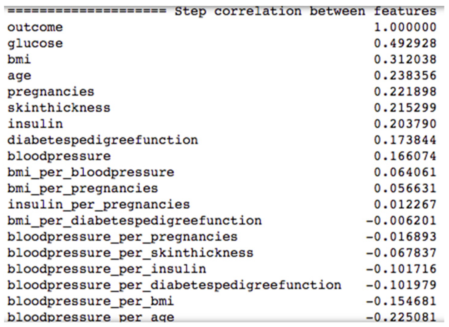
Figure 9 shows the top ten combination of features after applying the ANOVA model to the diabetes dataset.
Only using the feature blood pressure would be not very useful, as blood pressure per age would probably be more valuable for the prediction process. In
Figure 9, we can see that the raw feature blood pressure has a correlation of 0.166074 and the feature blood pressure per age has a higher absolute correlation value of 0.225081.
All other combinations of features have less correlation with the label outcome than the raw features, so for our machine learning algorithms, we used all the raw features and the combination feature blood pressure per age as input variables.
4.2.2. Human Resource Dataset
In
Figure 10, we can see the results of feature combination and the application of the ANOVA model to the human resource dataset. The use of the new feature average monthly hours per satisfaction level has more value for the prediction process than the raw feature average monthly hours because it has a higher correlation with the label left, respectively, 0.396279 and 0.070409. The same applies to the new feature satisfaction level per time spend company and average monthly hours per time spend company regarding the raw feature satisfaction level and average monthly hours, respectively.
For our machine learning algorithms, we used the raw features time spend company, average monthly hours, promotion last 5 years, salary, work accident and satisfaction level, and the combination feature average monthly hours per satisfaction level, average monthly hours per time spend company and satisfaction level per time spend company as input variables.
4.3. Evaluation Metrics
The predictive performance of the supervised techniques was assessed by the metrics
Accuracy in Equation (2),
Precision in Equation (3),
Recall in Equation (4),
F1-Score in Equation (5) and ROC-AUC-Score, where ROC stands for Receiver Characteristic Operator and AUC for Area Under the Curve.
TP,
TN,
FP and
FN stand for true positive, true negative, false positive and false negative, respectively. A true positive is an outcome wherein the model correctly predicts the positive class. Similarly, a true negative is an outcome where the model correctly predicts the negative class. A false positive is an outcome where the model incorrectly predicts the positive class. Similarly, a false negative is an outcome wherein the model incorrectly predicts the negative class.
Regarding the ROC-AUC-Score, ROC is a probability curve and AUC represents the degree or measure of separability. It expresses the extent to which the model is capable of distinguishing between classes. A higher AUC is positively correlated with the better performance of the model’s prediction of zero classes as zero and one classes as one.
For clustering unsupervised techniques, the predictive performance was assessed by the metrics Silhouette Score, Homogeneity Score, Completeness Score, V Measure Score, Adjusted Rand Score and Adjusted Mutual Info Score.
Silhouette Score, presented in Equation (6), is calculated using the mean intra-cluster distance (
a) and the mean nearest-cluster distance (
b) for each sample. It has values between −1 and 1, where the value 0 indicates overlapping clusters, and negative values indicate that the instance was assigned to the wrong cluster and the best values as close as possible to 1.
Homogeneity Score, shown in Equation (7), is useful to check whether the clustering algorithm meets an important requirement: a cluster should only contain samples belonging to a single class. It has values between 0 and 1, where 1 means that there is a perfect homogeneous classification.
Completeness Score, shown in Equation (8), has the purpose of checking whether all the data points that are members of a given class are elements of the same cluster. This varies between 0 and 1, where 1 means that all members of a class belong to the same cluster.
V Measure Score, shown in Equation (9), is the harmonic mean between homogeneity and completeness, varying between 0 and 1, with values of 1 meaning that there is a perfect homogeneous and complete classification. Beta is the ratio of weight attributed to homogeneity versus completeness.
Adjusted Rand Score, shown in Equation (10), is used to determine whether two cluster results are similar to each other. In formula (10),
RI stands for the Rand index, which calculates the similarity between two cluster results by taking all the points identified within the same cluster. It can have values between −1 and 1, where values close to 0 mean a random classification and values closer to 1 mean the best classification.
Adjusted Mutual Info Score, shown in Equation (11), is an adjustment of the Mutual Information (
MI) score to account for chance. It accounts for the fact that
MI is generally higher for two clusterings with a larger number of clusters regardless of whether there is actually more information shared.
U denotes label true and
V denotes label pred. It varies between −1 and 1, returning 1 when two partitions are identical or perfectly classified, while random partitions correspond to values close to 0.
4.4. Training and Testing
We tested 12 different algorithms to compare the predictive performance of various machine learning algorithms, as described in the following subsections. From the Scikit-learn library in Python, between supervised and unsupervised clustering techniques, along with the application of two unsupervised clustering algorithms (K-Means and BIRCH) for preprocessing three supervised techniques (Decision Tree, Logistic Regression and Naïve Bayes).
For all algorithms, three groups of the dataset were defined with training and testing percentages of 80% and 20%, 75% and 25%, and 70% and 30%, respectively.
4.4.1. Logistic Regression, Decision Tree, Naïve Bayes
We used all the default parameters values of the supervised Logistic Regression, Decision Tree and Naïve Bayes algorithms from the Scikit-learn library.
4.4.2. Support Vector Machine
There are two variants of the supervised Support Vector Machine algorithm, linear and non-linear, where the difference between them is the fact that the first can easily separate data with a linear line, and the second cannot.
For the
linear variant, default values from the Scikit-learn library were used except for parameter C, which is a regularization parameter [
37]. For large values of C, the optimization will choose a smaller-margin hyperplane to obtain all of the correctly classified training points. Conversely, a very small value of C will cause the optimizer to look for a larger-margin separating hyperplane, even if that hyperplane misclassifies more points. C parameter values of 0.1, 1 and 10 were defined.
For the
non-linear variant, default values were used, except for parameters C, gamma and kernel. The gamma parameter is used for non-linear hyperplanes, where higher values mean that the algorithm will try to exactly fit the training data [
37]. The kernel parameter is a method used to take data as input and transform into the required form of processing data. C and gamma parameter values of 0.1, 1 and 10 were defined, and the kernel parameter values of ‘linear’ and radial basis function (‘rbf’).
4.4.3. Random Forest
We used default values of the supervised random forest algorithm from the Scikit-learn library, except for the n_estimators, criterion and class_weight parameters. The N_estimators parameter is the number of trees needed in the algorithm that depends on the number of rows in the dataset. More rows means that more trees are needed [
38]. The criterion parameter is a function that measures the quality of a split in a tree. The class_weight parameter allows to specify the weights of each class in the case of an imbalanced dataset.
In the experiments, the n_estimators parameter assumes values of 10, 40, 70 and 100. The criterion parameter has the values of ‘gini’ and ‘entropy’, and the class_weight parameter values of ‘balanced’ and ‘balanced_subsample’.
4.4.4. K-Nearest Neighbors
We used the default values of the supervised clustering KNN algorithm from the Scikit-learn library, except for the n_neighbors parameter. The n_neighbors value indicates the count of nearest neighbors we want to select to predict the class of a given item [
39].
The n_neighbors parameter was defined with integer values from 1 to 9.
4.4.5. K-Means
We used the default values for the K-Means unsupervised clustering algorithm from the Scikit-learn library except for the n_clusters and n_init parameters. The n_clusters parameter is the number of clusters to form as well as the number of centroids to generate, while the n_init parameter is the number of times that the algorithm will be run with different centroid seeds [
40].
The n_clusters parameter was defined with integer values from to 2 to 5, and the n_init parameter was defined with integer values from 1 to 4.
4.4.6. Spectral Clustering
We used the default values of the unsupervised clustering Spectral Clustering algorithm from the Scikit-learn library, except for the n_clusters, n_init, gamma and assign_labels parameters. The n_clusters and n_init parameters have the same definition as from the K-Means algorithm, while the gamma parameter is the kernel coefficient and assign_labels is the strategy for assigning labels in the embedding space. The assign_labels parameter can take the values of ‘kmeans’ and ‘discretize’, where the first can be sensitive to initialization and the second is less sensitive to random initialization [
41].
The n_clusters parameter was defined with values of 2 and 3, n_init parameter was defined with values of 1 and 2, gamma parameter was defined with values of 0.01, 0.1 and 1, and assign_labels parameter was defined with values of ‘kmeans’ and ‘discretize’.
4.4.7. Mean Shift
For the unsupervised clustering Mean Shift algorithm, we used the default values from the Scikit-learn library, except for the bandwidth parameter which makes the Kernel Density Estimation (KDE) differ across different sizes. A small kernel bandwidth makes the KDE surface hold the peak for every data point, stating that each point has its cluster; on the other hand, a large kernel bandwidth results in fewer kernels of fewer clusters [
42].
The bandwidth parameter was defined with integer values from 2 to 5.
4.4.8. DBSCAN
For the unsupervised clustering DBSCAN algorithm, we used the default values from the Scikit-learn library except for the eps and min_samples parameters. The eps parameter is the maximum distance between two samples for one to be considered as in the neighborhood of the other, while the min_samples parameter is the number of samples in a neighborhood for a point to be considered as a core point [
43].
The eps parameter was defined with real values from 0.5 to 4 and min_samples parameter integer was defined with real values from 1 to 4.
4.4.9. BIRCH
For the unsupervised clustering BIRCH algorithm, we used the default values from the Scikit-learn library, except for the threshold, branching_factor and n_clusters parameters. For the threshold parameter, the radius of the subcluster obtained by merging a new sample and the closest subcluster should be lesser that the threshold, otherwise, a new subcluster is started. For the branching_factor parameter, if a new sample enters such that the number of subclusters exceeds the branching factor, then that node is removed and two new subclusters are added as the parents of the two split nodes. The n_clusters parameter is the number of clusters after the final clustering step which handles the subclusters from the leaves as new samples [
44].
The threshold parameter was defined with values of 0.1, 2 and 5, branching_factor parameter was defined with values of 20, 40 and 60 and n_clusters parameter was defined with values from 1 to 3.
5. Experimental Evaluation
In this section, we present the results obtained by applying the machine learning algorithms to the two datasets, following the approach described in the previous section. The Python source code used in the experiments is freely available at:
https://github.com/hfilipesilva/ml-algorithms (accessed on 7 April 2022).
5.1. Diabetes Dataset
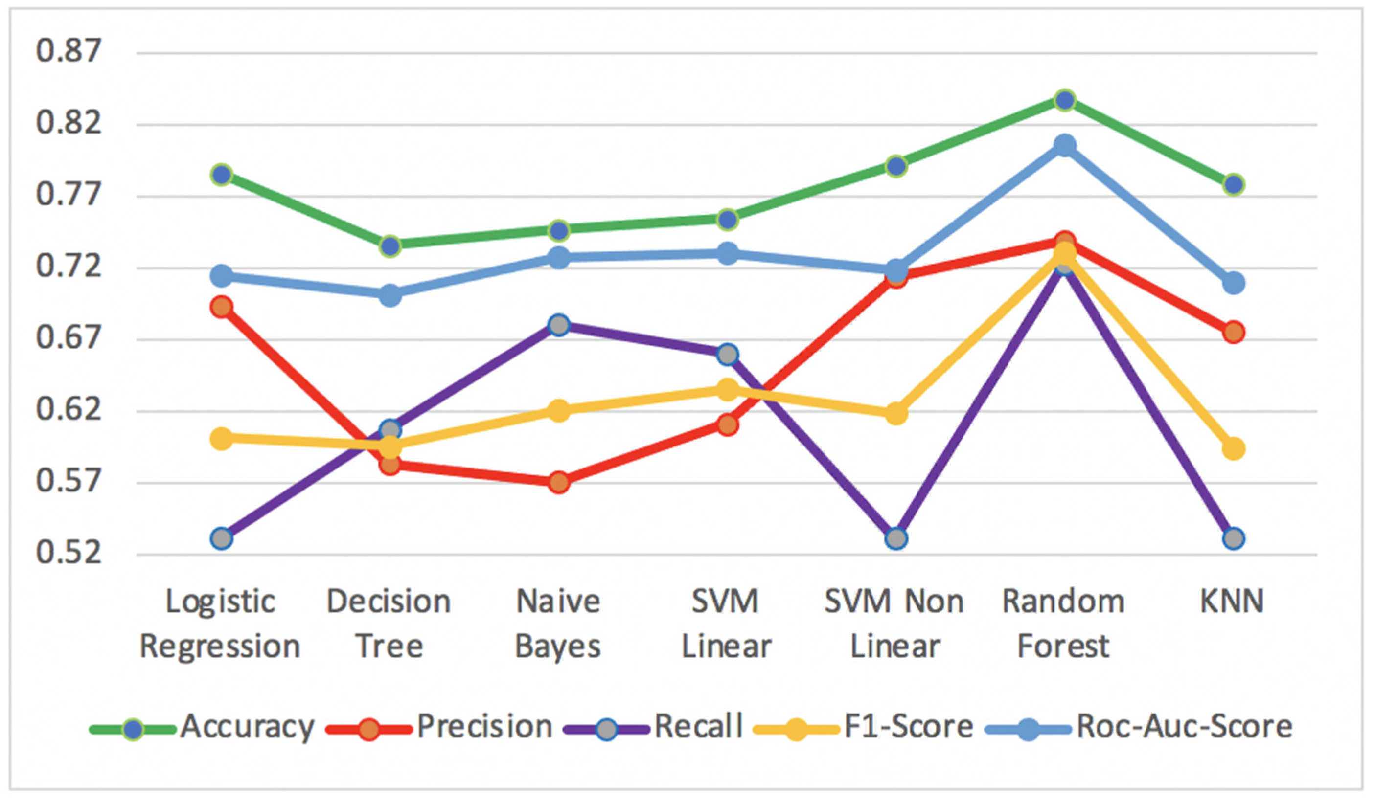
Figure 11 shows the best results of supervised algorithms for
Accuracy,
Precision,
Recall,
F1-Score and
ROC-AUC-Score metrics, applied to diabetes test dataset.
The Random Forest algorithm obtained the best performance results in all metrics, with Accuracy of 83.8%, Precision of 73.9%, Recall of 72.3%, F1-Score of 73.1% and ROC-AUC-Score of 80.6%. On the other hand, the Decision Tree algorithm presented the worst results for the metrics Accuracy of 73.6%, F1-Score of 59.6% and ROC-AUC-Score of 70.2%. The Naïve Bayes algorithm presented the worst result for Precision of 57.1%, while the Logistic Regression and KNN had the worst result for Recall with a value of 53.2%.
Figure 12 presents the results of the
Silhouette Score metric for unsupervised clustering algorithms applied to the diabetes test dataset.
We can see that the Spectral Clustering algorithm obtained the best Silhouette Score value of 84.8% while Mean Shift had the worst Silhouette Score value of 74.2%. The reason for which Mean Shift had the worst results can be justified by the fact that manually choosing the bandwidth can be non-trivial, and selecting a wrong value can lead to inferior results.
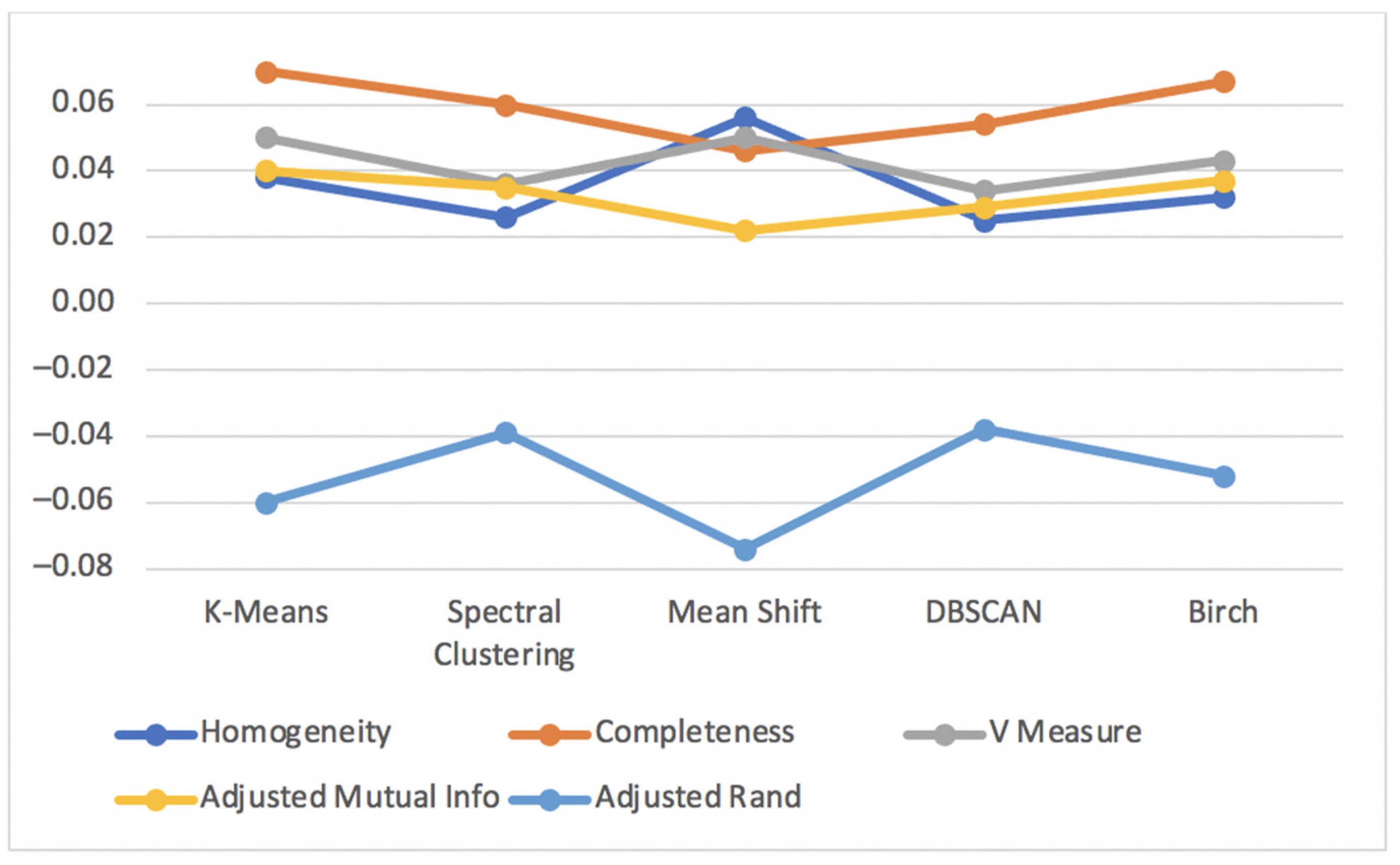
Figure 13 shows the results for the metrics
Homogeneity Score,
Completeness Score,
V Measure Score,
Adjusted Mutual Info Score and
Adjusted Rand Score for the unsupervised clustering algorithms applied to the diabetes test dataset.
All the previous metrics had considerably low values distant from the best value of 1 and −1 for every unsupervised clustering algorithm. This means that the values close to zero are the result of datapoints being randomly assigned in the clusters.
The best metric results of applying the two preprocessing unsupervised clustering techniques (K-Means and BIRCH) to Logistic Regression, Decision Tree and Naïve Bayes supervised algorithms for the diabetes test dataset are shown in
Table 1.
Overall, the result of applying unsupervised clustering techniques for preprocessing supervised algorithms was not improved performance, as can be seen in the metric results. However, for Logistic Regression, compared to Decision Tree and Naïve Bayes algorithms, preprocessing results were closer those without any preprocessing technique. Preprocessing Naïve Bayes had lower performance results compared to the original Naïve Bayes algorithm except for the Recall metric where it had a good result of 86.5% and 68.1%, respectively. Additionally, the preprocessing Decision Tree presented the best precision value of 59.2% compared to the original Decision Tree algorithm with a value of 55.7%.
5.2. Human Resource Dataset
Figure 14 shows the best results of supervised algorithms for
Accuracy,
Precision,
Recall,
F1-Score and
ROC-AUC-Score metrics applied to the human resource test dataset.
The Random Forest algorithm obtained the best performance results in the metrics with an Accuracy of 97.3%, Precision of 90.8%, F1-Score of 91.4% and ROC-AUC-Score of 95.1%. For the metric Recall, the SVM linear algorithm presented the best result of 94.7%. On the other hand, the SVM linear algorithm presented the worst results for the metric Accuracy of 79.7% and the metric Precision of 43.4%, while the Logistic Regression had the worst results for the metrics Recall of 24.3%, F1-Score of 36.5% and ROC-AUC-Score of 61.3%.
Figure 15 presents the results of the
Silhouette Score metric for the unsupervised clustering algorithms applied to human resource test dataset.
We can see that the BIRCH algorithm obtained the best Silhouette Score value of 72.6% while DBSCAN had the worst Silhouette Score value of 61.3%. The reason why DBSCAN had inferior results can be justified by the fact that in some cases, determining an appropriate distance of neighborhood (eps) is not easy and it requires domain knowledge. Additionally, if clusters are very different in terms of in-cluster densities, DBSCAN is not well suited to define clusters.
Figure 16 shows the results for the metrics
Homogeneity Score,
Completeness Score, V
Measure Score,
Adjusted Mutual Info Score and
Adjusted Rand Score for the unsupervised clustering algorithms applied to the human resource test dataset.
All the previous metrics had low scores which were distant from the best value of 1 for every unsupervised clustering algorithm, among which DBSCAN presented the worst results. As previously stated, DBSCAN can have a bad performance because it is normally difficult to determine an appropriate distance of neighborhood (eps) and if clusters are very different in terms of in-clusters densities.
The best metric results of applying the two preprocessing unsupervised clustering techniques (K-Means and BIRCH) to Logistic Regression, Decision Tree and Naïve Bayes supervised algorithms for human resource test dataset are shown in
Table 2.
The result of applying unsupervised clustering techniques as preprocessing of supervised algorithms considerably improved the performance, particularly for Logistic Regression algorithm, whereas Accuracy changed from 86.8% to 96%, Precision from 74% to 86.1%, Recall from 36.5% to 87.5%, F1-Score from 36.5% to 87.5% and ROC-AUC-Score from 61.3% to 93.1%. However, working with the Naïve Bayes algorithm, the metrics Recall, F1-Score, and ROC-AUC-Score did not show significant improvements.
In general, different datasets may impact the results because the best algorithm depends on the characteristics of the dataset, including its size, features as well as the different hyperparameters and tuning of them which obviously influence the results’ performance. This is the justification for which we have better performance results for the human resource dataset than for the diabetes dataset, as the first has a considerably higher number of instances and higher correlation feature values compared to the second.
6. Discussion of the Results
Each machine learning algorithm has its own pros and cons. For supervised techniques, the Random Forest algorithm presented the best results for both diabetes and human resource datasets as it uses the Ensemble Learning technique which does not require independency between attributes, and is more resilient to outliers and less impacted by noise [
24].
On the other hand, Logistic Regression showed lower results for some metrics, justified by the fact that no linearity exists between dependent and independent variables [
20]. The same happened for the SVM Linear algorithm where the frontier is a straight line and there may be difficulty in separating distinct classes [
21]. Naïve Bayes is also an algorithm that does not show the best performance because it implicitly assumes that all the features are mutually independent, which is almost impossible to happen [
23].
In the diabetes dataset, we can mention that it is more important to minimize false negatives because the condition is not detected when it is present, and the Recall metric, which involves the false negative, would be more important than the precision metric. In that sense, the Naïve Bayes and Random Forest algorithms presented the best Recall values.
For the human resource dataset, one can either privilege the reduction in false negatives, on retaining the best talents in the company, with the risk of retaining the worst employees, or privilege the reduction in false positives and having the worst employees leave the company with the risk of having a good employee leaving.
The diabetes dataset had lower metric values compared to the human resource dataset, which can be justified by the fact that we need to do more value imputations to the features, because of the presence of invalid values. Additionally, because the diabetes dataset has fewer instances compared to the human resource dataset and lower feature correlation values, this results in poor performance.
Generally, unsupervised techniques showed a lower performance in comparison with supervised techniques, because in the supervised technique, the algorithm learns from the training dataset by iteratively making predictions on the data and adjusting the correct answer. For unsupervised learning, in contrast, the algorithm works on their own to discover the inherent structure of unlabeled data. This is why supervised learning tends to be more accurate and have better performance results than unsupervised learning models.
For Naïve Bayes, the use of the preprocessing technique generally did not show improvements for the diabetes dataset or significant enhancements for the human resource dataset, because it is common knowledge that this algorithm is a bad estimator so the probability outputs are not to be taken too seriously. Another limitation of Naïve Bayes is the assumption of independent predictors. In real life, it is almost impossible that we obtain a set of predictors which are completely independent.
The application of unsupervised clustering preprocessing techniques for the diabetes dataset did not result in better performance, while in the human resource dataset, we can clearly see that it had a positive impact on the performance. This fact is justified because the human resource dataset has more instances than the diabetes dataset, and it is common knowledge that too little training data results in poor approximation. Additionally, because the human resource dataset has higher feature correlation values than the diabetes dataset, it has better performance. This demonstrates that the pre-classification of the human resource dataset made by the preprocessing unsupervised clustering techniques positively impacts the performance results.
7. Conclusions and Future Work
In this work, we used 12 algorithms among supervised and unsupervised clustering techniques applied to diabetes and human resource datasets for binary classification. We also applied the preprocessing technique to supervised algorithms, using unsupervised clustering techniques as this topic was little explored.
The knowledge generated by this work, namely the use of preprocessing supervised and unsupervised clustering algorithms, can contribute to the wider use and exploration of this technique so that the performance results of the application of supervised machine learning algorithms can be improved.
As future work, we intend to apply this technique to larger datasets to consolidate the promising benefits of using it. Additionally, we intend to use not only clustering also other unsupervised techniques as preprocessing to compare their impact on performance results. Finally, we also intend to use the cross-validation technique to test the model’s ability to predict new data that were not used in the estimation in order to flag problems such as overfitting or selection bias and to give insight into how the model will generalize into an independent dataset.


