Multi-Fidelity Low-Rank Approximations for Uncertainty Quantification of a Supersonic Aircraft Design

Abstract

Uncertainty quantification has proven to be an indispensable study for enhancing reliability and robustness of engineering systems in the early design phase. Single and multi-fidelity surrogate modelling methods have been used to replace the expensive high fidelity analyses which must be repeated many times for uncertainty quantification. However, since the number of analyses required to build an accurate surrogate model increases exponentially with the number of random input variables, most surrogate modelling methods suffer from the curse of dimensionality. As an alternative approach, the Low-Rank Approximation method can be applied to high-dimensional uncertainty quantification studies with a low computational cost, where the number of coefficients for building the surrogate model increases only linearly with the number of random input variables. In this study, the Low-Rank Approximation method is implemented for multi-fidelity applications with additive and multiplicative correction approaches to make the high-dimensional uncertainty quantification analysis more efficient and accurate. The developed uncertainty quantification methodology is tested on supersonic aircraft design problems and its predictions are compared with the results of single- and multi-fidelity Polynomial Chaos Expansion and Monte Carlo methods. For the same computational cost, the Low-Rank Approximation method outperformed both in surrogate modeling and uncertainty quantification cases for all the benchmarks and real-world engineering problems addressed in the present study.

1. Introduction

Over the past few decades, surrogate modelling or so-called meta-modelling has increasingly been employed for predicting results of physical computer simulations. Simulations can become prohibitively expensive when multiple realizations are required, as is the case with Uncertainty Quantification (UQ) or optimisation processes; the fast evaluation speed of surrogates makes them an attractive alternative, and have led to their wide acceptance and adoption in several engineering fields (see [1] for an overview of UQ with surrogate strategies). In the case of aerospace engineering design problems, where the failure allowance is quite limited, uncertainties for the design space variables are propagated through the output and have to be estimated accurately without any loss of reliability and within a reasonable period of time. In uncertainty quantification processes, even using surrogates for approximating physical phenomena can be quite time consuming and costly due to the need for many high-fidelity simulations to achieve reliable and robust designs, especially in the case of high-dimensional design optimisation problems. Thus, in an effort to further alleviate the computational burden of UQ, single-fidelity surrogates are extended to multi-fidelity versions by using additive and multiplicative correction approaches to reach an acceptable accuracy in limited time. Multi-fidelity models use different fidelity levels, which may significantly reduce the computational load and accelerate the computation. These models have been widely used to overcome the computational burden in uncertainty modelling and optimisation processes for complex simulations. The key feature behind the multi-fidelity methodology is to increase the accuracy of the intensively sampled low-fidelity simulations by exploiting a limited number of high-fidelity simulations, thus maintaining an acceptable computational cost. A comprehensive review for multi-fidelity methods in uncertainty quantification can be found in [2].

The main challenge in simulation-based realisations of engineering problems is the outgrowth in dimensionality, which increases the complexity and the computational time for calculating hyperparameters of the implemented surrogate. Particularly as dimensionality grows large, the Low-Rank Approximation (LRA) methodology is a prominent tool among surrogate modelling strategies model strategies, since the method models the response of the system as the sum of a smaller number of rank-one tensors, which are products of univariate functions. Since approximating the system of outputs is conducted using a smaller number of rank tensors, the number of unknown coefficients to be calculated grows only linearly with the input dimensions, which makes the method very advantageous, especially in high-dimensional cases. 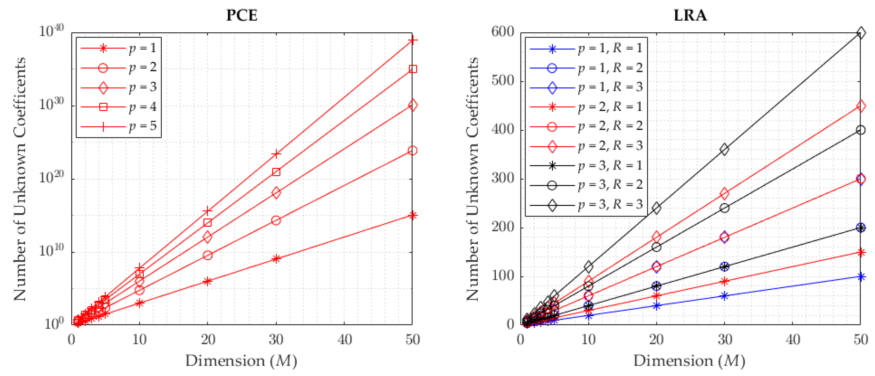The LRA method has been applied to several engineering disciplines recently, with particular focus on scaling with dimensionality; these topics include reliability-based optimisation [3,4,5], surrogate model strategies [6,7], uncertainty propagation [8,9,10], sensitivity analysis [11] and comparative studies with the Polynomial Chaos Expansion (PCE) method [12]. LRA is proposed as an alternative surrogate technique to the widely applied PCE. The number of unknown coefficients grows exponentially with the input size in the PCE method, whereas LRA has the advantage of only linearly increasing the number of coefficients with input size. In this study, LRA is therefore selected as a promising surrogate modelling method to overcome the burden of dimensionality as an alternative to PCE.

A number of related studies have been carried out in the literature. For instance, Blatman and Sudret [13] focused on uncertainty quantification and sensitivity analysis for high-dimensional problems; in particular, they calculated design variable sensitivities for different sizes of problems with the surrogate model using the Sparse Polynomial Chaos Expansion (SPCE) method. It was shown that SPCE was advantageous over PCE in terms of the number of analyses required to make an accurate prediction. In a following study, Blatmann and Sudret [14] combined SPCE with an adaptive algorithm to automatically determine the important polynomial coefficients. Comparing the results of the adaptive SPCE method with full PCE and stepwise SPCE demonstrated that the adaptive SPCE method could represent high-dimensional problems with fewer data. Konakli and Sudret [3] performed a reliability analysis for high-dimensional models using LRA, where the number of unknown coefficients increased linearly depending on the problem size. It was concluded that the LRA method outperformed the SPCE method while also using fewer analysis results. Papaioannou et al. [15] integrated the PCE method with the PLS method to approximate unknown orthogonal polynomial coefficients for high-dimensional problems and found that the PCE-PLS method provides more accurate estimations compared to the LRA method when a small number of simulations results are used. Recently, Son and Du [16] integrated the generalised dimension reduction algorithm with the PCE method for efficient uncertainty quantification of non-standard distribution types and Zuhal et al. [17] performed reliability analysis using the Kriging method integrated with the PLS algorithm instead of orthogonal polynomial-based methods for high-dimensional problems. Among multi-fidelity applications, Peterstorfer et al. [18] applied the multi-fidelity Monte Carlo (MFMC) method and Quaglino et al. [19] performed high-dimensional uncertainty quantification studies using the multi-level Monte Carlo method.

High-fidelity engineering simulations are usually computationally expensive, and uncertainty quantification processes using high-fidelity engineering models struggle with extreme computational cost. Multi-fidelity methods leverage both high-fidelity and low-fidelity data to reduce the high computational or experimental costs by achieving high accuracy simultaneously. As multi-fidelity surrogate modelling methods reduce the computational cost of simulations with an acceptable accuracy, this approach can be a remedy for uncertainty quantification processes [2]. In uncertainty quantification studies, orthogonal polynomial-based surrogate models such as multi-fidelity PCE [20] and SPCE [21] can be preferred since they successfully represent the general behaviour of computational models. In [20,21] studies, additive and multiplicative correction terms were used to extend the multi-fidelity versions of PCE and SPCE. In addition, there are studies in which multi-fidelity extensions of these methods are made with the Gaussian process such as [22]. Other widely used multi-fidelity methods are kernel-based methods such as the multi-fidelity Gaussian process [23], coKriging [24], and Stochastic Radial Basis function [25]. These methods are preferred in optimisation studies due to their success in capturing local properties and are also used in uncertainty analysis. In addition, there are methods such as Polynomial Chaos-coKriging [26] and Sparse Polynomial Chaos-Kriging [27], which combine the ability to capture global features of orthogonal-based methods with the ability to capture local features of kernel-based methods.

Regarding the uncertainty quantification for a low-boom aircraft design, the effects of uncertainties in flight conditions and atmospheric profile at the sonic boom level were studied by West et al. [28] using a mixed uncertainty quantification and second-order probability method; they performed the uncertainty quantification for flow analysis through a PCE surrogate model, which significantly increased the computational demand. Philips and West [29] and Nikbay et al. [30] studied the effect of aeroelastic impacts on sonic boom using the non-intrusive PCE method. Nikbay et al. [30] examined the effect of uncertainties due to the material properties on the sonic boom and reduced the number of uncertain parameters by performing sensitivity analysis. Rallabhandi et al. [31] used the PCE method for uncertainty calculation and performed robust low boom design using atmospheric uncertainties. West and Philips [32] measured the uncertainty in the sonic boom level using the results of a small number of expensive analyses and based on three different fidelity levels with the multi-fidelity PCE method. Tekaslan et al. [20] performed low-dimensional sonic boom uncertainty analysis using MFMC and MF-PCE methods. To the best of the authors’ knowledge, the LRA method has not been applied to any engineering problems in the aviation field yet and the LRA method has not been implemented within a multi-fidelity modelling approach. The authors implemented the LRA method into an uncertainty quantification process for sonic boom prediction and further developed a novel multi-fidelity approach of the LRA method which is called the MF-LRA method in this paper. This new approach is comprehensively compared with the multi-fidelity PCE method. In addition, it is observed that the literature lacks high-dimensional numerical multi-fidelity benchmark problems; so as a contribution of the authors, a new multi-fidelity extension of the Sobol’-Levitan function is implemented and presented in this study.

Within this perspective, this paper first aims to present a comprehensive performance assessment by constructing a multi-fidelity extension to a Low-Rank Approximation and comparing the results with a competing approach of multi-fidelity Polynomial Chaos Expansion for multi-fidelity analytical test cases. Then, the present approach is used for the uncertainty quantification of high-dimensional supersonic aircraft design problems within an application-oriented framework.

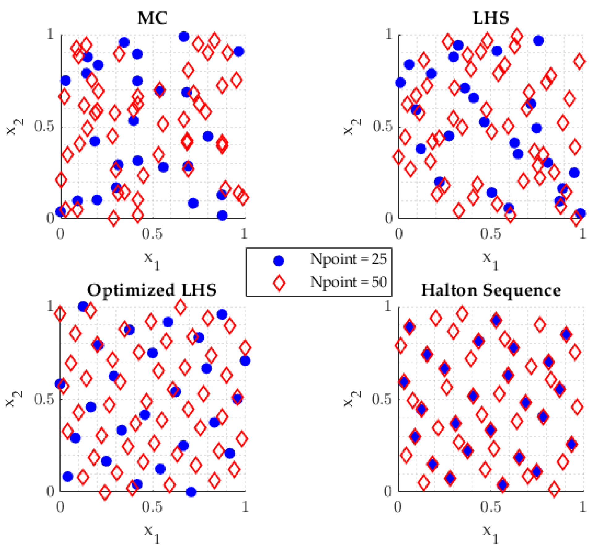
The remainder of the paper is as follows: In Section 2, some of the basic properties and concepts are introduced for the present methods and the details of the multi-fidelity extension of the surrogates are explained. In Section 3, the details of the computational experiment (e.g., the selected sampling strategy for the design of experiments (DoE)) are given; accuracy metrics and performance results for both analytical and high-dimensional engineering problem test cases are also demonstrated. In the final section, the results are discussed and current challenges along with the recommendations for further investigations are presented.

2. Methods

In this section, the concepts and basic terms are explained for the Polynomial Chaos Expansion and Low-Rank Approximation surrogate modelling strategies. For a more elaborate introduction and detailed descriptions of the models, one can refer to the following references within the uncertainty quantification framework [33,34].

2.1. Polynomial Chaos Expansion

The PCE method is based on the principle that a computational model can be obtained by an infinite series expansion of orthogonal polynomials as in Equation (1). In this equation, $\mathcal{M}$ represent the computational model with the outputs of the system, $\mathbf{Y}=\{Y_1,\cdots ,Y_N\}$, being dependent on the variables $\mathbf{X}=\{X_1,\cdots ,X_M\}$.

$$\mathcal{M}\left(\mathbf{X}\right)=\sum _{j=0}^{\infty }{\alpha }_j{\mathsf{\Psi }}_j\left(\mathbf{X}\right)$$

(1)

From a computational point of view, the infinite series should appropriately be truncated. The PCE method suggests that, as in Equation (2), the computational model can be expressed with a small error, $\epsilon$, by using a $P+1$ terms in the series expansion:

$$\mathcal{M}\left(\mathbf{X}\right)\approx {\mathcal{M}}^{PCE}\left(\mathbf{X}\right)\cong \sum _{j=0}^P{\alpha }_j{\mathsf{\Psi }}_j\left(\mathbf{X}\right)+\epsilon$$

(2)

The $\alpha$ terms in Equation (2) indicate unknown coefficients, and the $\mathsf{\Psi }$ vector are the multivariate orthogonal terms. Multivariate orthogonal (${\mathsf{\Psi }}_i\left(\mathbf{X}\right)$) terms are obtained by multiplying univariate orthogonal polynomials (${\psi }_{m_i^j}\left(x\right)$) as in Equation (3). $m_i^j$ in this equation represents the index of the univariate Hermite polynomial.

$${\mathsf{\Psi }}_j\left(\mathbf{X}\right)=\prod _{i=1}^M{\psi }_{m_i^j}\left(x_i\right)$$

(3)

Depending on the probability distribution of the inputs of the computational model, different orthogonal polynomials may be used. Legendre polynomials are used for uniformly distributed inputs and Hermite polynomials are used for normally distributed inputs. The definition of the first few two-dimensional Hermite polynomials is expressed in terms of the standard variable $\xi$ as in Equation (4) [35].

$$\begin{array}{cc}\hfill {\mathsf{\Psi }}_0\left(\mathit{\xi }\right)& ={\psi }_0\left({\xi }_1\right){\psi }_0\left({\xi }_2\right)=1\hfill \\ \hfill {\mathsf{\Psi }}_1\left(\mathit{\xi }\right)& ={\psi }_1\left({\xi }_1\right){\psi }_0\left({\xi }_2\right)={\xi }_1\hfill \\ \hfill {\mathsf{\Psi }}_2\left(\mathit{\xi }\right)& ={\psi }_0\left({\xi }_1\right){\psi }_1\left({\xi }_2\right)={\xi }_2\hfill \\ \hfill {\mathsf{\Psi }}_3\left(\mathit{\xi }\right)& ={\psi }_2\left({\xi }_1\right){\psi }_0\left({\xi }_2\right)={\xi }_1^2-1\hfill \\ \hfill {\mathsf{\Psi }}_4\left(\mathit{\xi }\right)& ={\psi }_1\left({\xi }_1\right){\psi }_1\left({\xi }_2\right)={\xi }_1{\xi }_2\hfill \\ \hfill {\mathsf{\Psi }}_5\left(\mathit{\xi }\right)& ={\psi }_0\left({\xi }_1\right){\psi }_2\left({\xi }_2\right)={\xi }_2^2-1\hfill \end{array}$$

(4)

There are different methods such as the Smolyak sparse grid [36], random sampling [37], tensor product quadrature [38] and regression to calculate unknown $\alpha$ coefficients. The methods other than the regression method are spectral projection methods, which consist of projecting the computational model responses against each basis function using inner products. Unlike projection methods, an arbitrary number of results from the analysis can be used to calculate unknown coefficients in the regression method. In the present work, the regression method is used to calculate the unknown coefficients. The PCE series expansion in Equation (2) is expressed in matrix notation as in Equation (5):

$$\mathbf{Y}=\mathsf{\Psi }\mathit{\alpha }+\mathit{e}$$

(5)

The expressions in Equation (5) are expressed in matrix form as in Equation (6) where $\mathit{e}$ are the residuals.

$$\mathbf{Y}=\left[\begin{array}{c}{Y}_1\\ Y_2\\ ⋮\\ Y_{N_s}\end{array}\right],\mathsf{\Psi }=\left[\begin{array}{cccc}1& {\mathsf{\Psi }}_1\left({\mathbf{X}}_{\mathbf{1}}\right)& \dots & {\mathsf{\Psi }}_p\left({\mathbf{X}}_{\mathbf{1}}\right)\\ 1& {\mathsf{\Psi }}_1\left({\mathbf{X}}_{\mathbf{2}}\right)& \dots & {\mathsf{\Psi }}_p\left({\mathbf{X}}_{\mathbf{2}}\right)\\ ⋮& ⋮& \ddots & ⋮\\ 1& {\mathsf{\Psi }}_1\left({\mathbf{X}}_{{\mathbf{N}}_{\mathbf{s}}}\right)& \dots & {\mathsf{\Psi }}_p\left({\mathbf{X}}_{{\mathbf{N}}_{\mathbf{s}}}\right)\end{array}\right],\mathit{\alpha }=\left[\begin{array}{c}{\alpha }_1\\ {\alpha }_2\\ ⋮\\ {\alpha }_{N_s}\end{array}\right],\mathbf{e}=\left[\begin{array}{c}{e}_1\\ e_2\\ ⋮\\ e_{N_s}\end{array}\right]$$

(6)

The unknown coefficients can be expressed as in Equation (7) with the ordinary least square method:

$$\mathit{\alpha }={\left({\mathsf{\Psi }}^T\mathsf{\Psi }\right)}^{-1}{\mathsf{\Psi }}^T\mathbf{y}$$

(7)

With the calculation of unknown coefficients, the estimation for a new design variable can be obtained as in Equation (8).

$${\mathcal{M}}^{PCE}\left(\mathbf{X}\right)=\mathsf{\Psi }\mathit{\alpha }$$

(8)

The number of terms to be included in the polynomial expansion in Equation (2) is calculated as in Equation (9). In this equation, M represents the number of random variables and p represents the maximum degree of the one-dimensional orthogonal polynomial.

$$N_s=P+1=\frac{(M+p)!}{M!p!}$$

(9)

In order to obtain the unknown polynomial coefficients correctly, the required number of analyses ($N_s$) must be greater than the number of polynomial coefficients $P+1$. Hosder et al. [39] suggest that $N_s=2(P+1)$ should be the number of analyses required for accurate surrogate modelling. It is observed from Equation (9) that the number of analyses required to obtain the correct result increases exponentially depending on the size of the problem.

In order to set up the PCE surrogate model, it is necessary to determine the degree of polynomial to be used. As the degree of polynomial increases, the number of unknowns also increases; this improves accuracy of the representation but also increases the number of required model evaluations. It is therefore necessary to determine the optimal maximum polynomial order. For the test cases in the present work, this is conducted by searching a limited interval through the use of an n-fold cross-validation metric.

2.2. The Low-Rank Approximation Method

The LRA method is constructed as an alternative to the PCE method to overcome the curse of dimensionality for high-dimensional problems [12]. As discussed in the previous section, in the PCE methodology, the response of the problem is expanded onto a basis of orthonormal multivariate polynomials. LRA instead relies on a tensor product form of multivariate basis, which accelerates the solution procedure of the unknown coefficients. In this study, LRA implementations are conducted using UQLab, an open-source MATLAB toolbox for uncertainty quantification [40].

A computational model ${\mathcal{M}}^{LRA}$, which represents a surrogate, maps the input variables to the response of the system. $\mathcal{M}$ represents the physical behaviour of the system outputs, which are denoted as $\mathbf{Y}=\{Y_1,\cdots ,Y_N\}$ and correspond to the variables $\mathbf{X}=\{X_1,\cdots ,X_M\}$. By considering a rank-one function of the input vector $\mathbf{X}$ in Equation (10),

$$w\left(\mathbf{X}\right)=\prod _{i=1}^M{v}^{\left(i\right)}\left(X_i\right)$$

(10)

where w is product of univariate component of the input variables and the LRA model in general form is given in Equation (11):

$$\mathcal{M}\left(\mathbf{X}\right)\approx {\mathcal{M}}^{LRA}\left(\mathbf{X}\right)\cong \sum _{l=1}^R{b}_l\left(\prod _{i=1}^M{v}_l^{\left(i\right)}\left(X_i\right)\right)$$

(11)

In this expression of the model, $v_l^{\left(i\right)}$ are univariate functions of $X_i$ in the $l^{th}$ rank-one component and $\{b_l,l=1,2,\cdots ,R\}$ are scalars defined as weighing factors. To approximate the response of the system, univariate functions $v_l^{\left(i\right)}$ are expanded onto the polynomial basis $\{{\psi }_k^{\left(i\right)},k\in \mathbb{N}\}$ that is orthonormal with respect to $f_{x_i}$.

$$\langle {\psi }_j^{\left(i\right)},{\psi }_k^{\left(i\right)}\rangle ={\int }_{{\mathcal{D}}_{x_i}}{\psi }_j^{\left(i\right)}{\psi }_k^{\left(i\right)}x\left(i\right)f_{x_i}\left(x_i\right)d{x}_i={\delta }_{jk}$$

(12)

${\mathcal{D}}_{x_i}$ represents a particular input variable while ${\delta }_{jk}$ is the Kronecker delta, which is 1 if $j=k$ and otherwise equal to 0. Accordingly, the polynomial basis representation leads to the equation,

$$v_l^{\left(i\right)}\left(X_i\right)=\sum _{k=0}^{p_i}{z}_{k,l}^{\left(i\right)}{\psi }_k^{\left(i\right)}\left(X_i\right)$$

(13)

where ${\psi }_k^{\left(i\right)}$ is the k-th degree univariate polynomial in the i-th input variable, $p_i$ is the maximum degree of ${\psi }_k^i$, and $z_{k,l}^i$ is the coefficient of ${\psi }_k^i$ in the l-th rank-one term. Then, using this expression in the LRA model in Equation (14),

$${\mathcal{M}}^{\mathrm{LRA}}\left(\mathbf{X}\right)=\sum _{l=1}^R{b}_l\left(\prod _{i=1}^M\left(\sum _{k=0}^{p_i}{z}_{k,l}^{\left(i\right)}{\psi }_k^{\left(i\right)}\left(X_i\right)\right)\right)$$

(14)

the approximation for the system outputs is obtained. Two stages are needed to construct LRA; one is to define the polynomial basis in each dimension and the other is to determine the polynomial coefficients. As indicated in the previous section, Legendre polynomials are used for uniformly distributed inputs, and Hermite polynomials are used for normally distributed inputs. While several algorithms have been implemented for computing unknown coefficients in the related literature, in this work the alternated least-squares (ALS) minimisation scheme is used [41]. The key feature of the ALS minimisation method is that the coefficients are obtained within each dimension while keeping the coefficients in remaining dimensions constant, thus accelerating the solution process.

The construction of the LRA methodology is based on both correction and updating steps in which the rank–one tensor is created in correction and the weighting factors are subsequently determined in the updating stages [12]. In the correction stage, assuming that ${\mathcal{R}}_r$ represents the residual after the r-th iteration,

$${\mathcal{R}}_r\left(\mathbf{X}\right)=\mathcal{M}\left(\mathbf{X}\right)-{\mathcal{M}}_r^{LRA}\left(\mathbf{X}\right)$$

(15)

the solution procedure is initiated by ${\mathcal{M}}_0^{LRA}\left(\mathbf{X}\right)=0$. By using the ALS scheme, the minimisation problem;

$${\mathbf{z}}_r^{\left(j\right)}=\underset{\zeta \in {\mathbb{R}}^{p_j}}{argmin}\parallel {\mathcal{R}}_{r-1}-\prod _{i\ne j}{v}_r^{\left(i\right)}\sum _{k=0}^{p_j}{\zeta }_k^{\left(i\right)}{\psi }_k^{\left(j\right)}{\parallel }_{ϵ}^2,j=1,2,\cdots ,M.$$

(16)

turns into smaller minimisation problems, with each considering the coefficients of one dimension. Correction step starts with arbitrary values of $\{v_r^{\left(i\right)},i=1,2,\cdots ,M\}$. The algorithm stops when the maximum iteration is reached or the error between iterations is smaller than the predetermined limit. As suggested by Konakli and Sudret [11] the maximum number of iterations is taken as $Imax=50$, while the predetermined limit for the error between iterations should be less than ${10}^{-6}$. Accordingly, in the updating step, the coefficients are obtained by solving the minimisation as in Equation (17).

$$\mathbf{b}=\underset{\beta \in {\mathbb{R}}^r}{argmin}{∥\mathcal{M}-\sum _{l=1}^r{\beta }_l{w}_l∥}_{ϵ}^2$$

(17)

The LRA methodology can be summarised in two steps; the correction stage consists of solving M minimisation problems of size $\{p_i+1,i=1,2,\cdots ,M.\}$ while the updating stage considers a minimisation of a smaller problem with size corresponding to rank r in the approximation.

The correction and updating stages are continued when the optimal rank and polynomial degree satisfies the predetermined error threshold between the iterations. Optimal rank is determined based on n-fold cross validation error. It is important to note here that the number of the unknowns in Equation (14) is $R·{\sum }_{i=1}^M(p_i+1)$, which grows linearly with the input dimensions, making the LRA a more preferred approach when compared to the PCE method, especially for high-dimensional problems. One can see that, by disregarding the redundant parameters, the number of unknown coefficients is drastically reduced when compared to PCE in Equation (2). Figure 1 demonstrates the advantage of LRA, with the number of unknown coefficients increasing linearly with problem dimensionality; in contrast, PCE demonstrates an exponential trend, making it prohibitively expensive for high dimensional problems.

For a conceptual comparison of the surrogates considered here; the general format of models are represented in

Table 1. The general form of the surrogates.

Model Name	Model Shape
Polynomial Chaos Expansion	${\sum }_{j=0}^P{\alpha }_j{\mathsf{\Psi }}_j\left(X\right)$
Low-Rank Approximation	${\sum }_{l=1}^R{b}_l{\prod }_{i=1}^M{v}_l^{\left(i\right)}\left(X_i\right)$

. As summarised in this table, both surrogate strategies belong to the family of univariate polynomials.

2.3. Multi-Fidelity Extension of PCE and LRA

In multi-fidelity surrogate modelling, by taking advantage of the low-cost computation of the low-fidelity model data, the accuracy of the surrogate model is increased by integrating a limited number of high-fidelity data with a larger number of low-fidelity data. In the present study, the additive and multiplicative correction approaches are implemented in order to use the orthogonal polynomial-based PCE and LRA methods in multi-fidelity surrogate modelling. Ng et al. [42] used the PCE method with the additive and multiplicative correction approach for multi-fidelity surrogate modelling and demonstrated that more accurate results were achieved with the correction approach as compared with those of the single-fidelity model. To the best of the authors’ knowledge, a multi-fidelity surrogate modelling study in which the LRA method is used does not exist. Thus, the authors are encouraged to investigate the cost and accuracy performance of the LRA method in multi-fidelity modelling in the present study where the LRA method is extended for multi-fidelity surrogate modelling with additive and multiplicative approaches similar to the PCE method.

The present multi-fidelity surrogate strategy is based on modelling the difference between low-fidelity $f_{lf}\left(\mathbf{X}\right)$ and high-fidelity $f_{hf}\left(\mathbf{X}\right)$ model responses. The additive and multiplicative correction approach essentially shifts and scales the low-fidelity model according to the high-fidelity model results. The additive ($C_a\left({\mathbf{X}}_{hf}\right):\mathbf{X}\to Y$) and multiplicative correction ($C_m\left({\mathbf{X}}_{lf}\right):\mathbf{X}\to Y$) functions are defined as in Equations (18) and (19), respectively.

$$C_a\left({\mathbf{X}}_{hf}\right)=f_{hf}\left({\mathbf{X}}_{hf}\right)-f_{lf}\left({\mathbf{X}}_{hf}\right)$$

(18)

$$C_m\left({\mathbf{X}}_{hf}\right)=\frac{f_{hf}\left({\mathbf{X}}_{hf}\right)}{f_{lf}\left({\mathbf{X}}_{hf}\right)}$$

(19)

Using the combination of the correction functions, the multi-fidelity surrogate model, which shifts the low-fidelity prediction to high-fidelity data, is given in Equation (20).

$${\tilde{f}}_{mf}\left(\mathbf{X}\right)=\gamma [{\tilde{f}}_{lf}\left(\mathbf{X}\right)+{\tilde{C}}_a\left(\mathbf{X}\right)]+(1-\gamma ){\tilde{f}}_{lf}\left(\mathbf{X}\right){\tilde{C}}_m\left(\mathbf{X}\right)$$

(20)

In Equation (20), the $\tilde{}$ expression represents the surrogate model, while ${\tilde{f}}_{lf}\left(\mathbf{X}\right)$, ${\tilde{C}}_a\left(\mathbf{X}\right)$, and ${\tilde{C}}_m\left(\mathbf{X}\right)$ represent the surrogate models established for the low fidelity, additive function, and multiplicative function results, respectively. Here, ${\tilde{f}}_{mf}\left(\mathbf{X}\right)$ refers to the multi-fidelity surrogate model established by the combination of these surrogate models. In this context, $\gamma$ is called the weight coefficient and represents the weights of the additive and multiplicative models. The authors of [42] proposed an expression for $\gamma$ that can be calculated using the norm of the additive and multiplicative correction in the mean-square sense as in Equation (21):

$$\gamma =\frac{\langle {\tilde{C}}_a^2\left(\mathbf{X}\right)\rangle }{\langle {\tilde{C}}_a^2\left(\mathbf{X}\right)\rangle +\langle {\tilde{C}}_m^2\left(\mathbf{X}\right)\rangle }$$

(21)

3. Computational Experiments

Real-world engineering applications are expected to be solved within limited computational budgets. For uncertainty quantification studies, the number of simulations increases drastically when propagating the input uncertainties to an output response through time consuming simulation processes. On the contrary, very limited amount of high fidelity data may be available to be used in surrogate modelling and uncertainty quantification studies. In this study, the goal is to investigate the cost and accuracy performance of the LRA method in multi-fidelity modelling with respect to the PCE method; in order to isolate the effects of surrogate performance, all accompanying computational strategies are kept the same, including design of experiments, local/global accuracy metrics, UQ metrics, and fidelity cost assignment criteria.

• Design of Experiments (DoE): Halton Sampling
  The key component of the surrogate modelling process is the design of experiments for the simulations. As already known from the associated studies, surrogate model predictions strictly depend on the applied design of experiments (DoE) set. In this study, several widely used DoE sampling types are demonstrated for a reliable performance assessment of the considered surrogates. To incorporate all the characteristics of the data over the sampling space, samples must be distributed homogeneously as much as possible. If this is achieved, the performance of the surrogate can be evaluated without the biased effect of the selected sampling strategy. With this in mind, Monte Carlo (MC) [43], Latin Hypercube (LHS) [44], Optimized Latin Hypercube (OLHS) [45] and Halton sequence (HS) sampling [46] strategies are compared in Figure 2 to visualise behavioural differences for several conventional sampling types.
  As indicated in the two-dimensional sampling strategy visualisations, Latin Hypercube sampling has the ability to fill the design space successfully. In contrast, Monte Carlo sampling may have some accumulated data areas that may result in learning deficits for the implemented surrogate model. The Halton sequence distributes the samples homogeneously over the design space. As the number of samples is increased, HS keeps the previous sampling set the same, while adding the new samples homogeneously distributed to the vacant regions of the design space. In the present work, Halton sequence is therefore selected as a DoE strategy in an effort to prevent potential bias effects from the sampling strategy.
• Local/Global accuracy metrics:
  In order to compare the accuracy of surrogate models, error metrics are calculated using the predicted values of the surrogate models and their corresponding analytical results at the same test points. The proposed metrics are selected to offer a comprehensive assessment of the surrogates both in terms of local and global characteristics of the modelling ability of the real functions. These metrics include coefficient of determination ($R^2$), root-mean square error ($RMSE$), and maximum absolute error ($MAE$); their formulas and normalised versions are later given in Equations (22)–(24).
  The coefficient of determination is a statistical measure of how well the regression estimate converges to the actual data points. $R^2$ takes a value between 0 and 1, with a high $R^2$ value indicating that the model fits well with the data used. Using the test data-set, the formulation is expressed as follows, where $\overline{y}$ is the mean of test data-set, $y_i$ is the exact value of the function and ${\widehat{y}}_i$ represents the surrogate model prediction.

  $$R^2=1-\frac{{\sum }_{i=1}^N{\left(y_i-{\widehat{y}}_i\right)}^2}{{\sum }_i^N{\left(y_i-\overline{y}\right)}^2}$$

  (22)
  The $RMSE$ metric expresses the standard deviation of the prediction error and measures how well the predicted values match the actual values in absolute terms. The $RMSE$ value ranges from 0 to ∞, with smaller values indicating that the method makes a more accurate prediction. In this respect, $RMSE$ is a global accuracy metric that represents the difference between the true value and the surrogate model value. It is used in the study to measure the success of the methods in capturing global behaviour. Using a test data-set, the formulation is expressed as in Equation (23).

  $$\begin{array}{c}RMSE=\sqrt{\frac{1}{N}\sum _{i=1}^N{\left(y_i-{\widehat{y}}_i\right)}^2}\\ NRMSE=\frac{RMSE}{\left(y_{max}-y_{min}\right)}\end{array}$$

  (23)
  The maximum absolute error value represents the greatest difference in the design space between the surrogate model prediction and the actual value. $MAE$ is frequently used in the literature to measure the prediction success of the surrogate model locally, and in this study, it is used to quantify how accurately the surrogate models capture the local features. The formulation is expressed using a test data-set as follows,

  $$\begin{array}{c}MAE=max\left(\left|y_i-{\widehat{y}}_i\right|\right)\\ NMAE=\frac{MAE}{\left(y_{max}-y_{min}\right)}\end{array}$$

  (24)
  The proposed assessment metrics might show different characteristics, as global accuracy may differ from local accuracy. In order to present a comprehensive performance evaluation of the surrogates, two different type of metrics are considered. A surrogate model’s ability to capture both local and global characteristics needs to be evaluated. For example, when considering a search for an optimum or any other local response of the surrogate, the $MAE$ has crucial importance to ensure that the model has no local deficits. At the same time, to facilitate an efficient evaluation of the surrogate performance, some kind of a compromise has to be observed between local and global accuracy of the models.
• Uncertainty quantification (UQ) metrics:
  Evaluation of the uncertainty quantification results is performed using the probability density function. In engineering problems, the terms mean, standard deviation, skewness and kurtosis, which express the behaviour of the density function, are used to numerically compare the results of the uncertainty quantification. The mean ($\overline{y}$) is the general tendency of the response based on the variation of the uncertain variables, and the standard deviation($\sigma$) refers to the variation in the analysis program’s response based on the distribution of the uncertain variable. The mean and standard deviation formulas are given in Equation (25), where N represents the number of responses.

  $$\overline{y}=\frac{{\sum }_{i=1}^N{y}_i}{N},\widehat{\sigma }=\sqrt{\frac{{\sum }_{i=1}^N{(y_i-\overline{y})}^2}{N-1}}$$

  (25)
  Skewness is a measure of the asymmetry of the probability density of response relative to the mean and is calculated as in Equation (26). Kurtosis, on the other hand, expresses a measure of whether the data contain an abundance of outliers or lack of outliers relative to a normal distribution and is calculated as in Equation (26).

  $$\mathrm{Skewness}=\frac{{\sum }_{i=1}^N{(y_i-\overline{y})}^3}{(N-1)·{\widehat{\sigma }}^3},\mathrm{Kurtosis}=\frac{{\sum }_{i=1}^N{(y_i-\overline{y})}^4}{(N-1)·{\widehat{\sigma }}^4}$$

  (26)
• Fidelity cost assignment criteria:
  Multi-fidelity surrogate assessments are usually depicted by using a constant number of low-fidelity analyses and adding high-fidelity data as necessary. Since design problems have to be solved with limited computational budget to complete the process within a reasonable amount of time, dominance of low fidelity data is more convenient. Preliminary cost assignment is determined by using single-fidelity performance results, which means the data are fixed for low-fidelity cases when an initial convergence occurs. Then, the number of low-fidelity runs are kept constant and high-fidelity runs are increased to a level when an acceptable convergence is reached by the multi-fidelity surrogate.

4. Numerical Results

Performances of the surrogate models are assessed by both analytical test cases and real-world engineering problems.

4.1. Analytical Test Cases

Beginning with analytical test cases, the primary purpose of this paper is to present performance assessments of the considered surrogates to determine whether they meet the requirements of a reliable uncertainty quantification process. This section therefore provides the analytical definitions of the selected benchmark functions to be used in the uncertainty quantification studies. These benchmarks are described for varying numbers of dimensions.

4.1.1. Problem 1: Park (1991) Function (4-D)

The Park (1991) function is a 4-D benchmark problem. It has been extended by Xiong [48] for multi-fidelity problems, and the high- and low-fidelity versions are given in Equations (27) and (28), respectively. For the presented problem, the design variable domain is defined as $x_i\in [0,1)$.

$$f_{hf}\left(\mathbf{x}\right)=\frac{x_1}{2}\left[\sqrt{1+\left(x_2+x_3^2\right)\frac{x_4}{x_1^2}}-1\right]+\left(x_1+3x_4\right)exp\left[1+sin\left(x_3\right)\right]$$

(27)

$$f_{lf}\left(\mathbf{x}\right)=\left[1+\frac{sin\left(x_1\right)}{10}\right]f\left(\mathbf{x}\right)-2x_1+x_2^2+x_3^2+0.5$$

(28)

Uncertainty quantification is performed using a surrogate model, and model training is conducted to determine the best parameters for the surrogate model to be used.

A surrogate model was created for single and multi-fidelity versions of the PCE and the LRA methods using different numbers of high-fidelity simulations results. The global and local accuracy metrics calculated at ${10}^5$ test points and the results of the performed surrogate models are demonstrated in Figure 3.

As is observed from Figure 3, an accurate surrogate model can be established by using the LRA method with only 10 high-fidelity simulations results. In contrast, when the PCE method is considered, a locally and globally accurate surrogate model can be established within approximately 35 high-fidelity simulations results. For the same simulation conditions (i.e., sampling strategy and number of simulations results), the PCE method therefore requires three times more data to achieve similar accuracy. In addition, by using the MF-PCE and MF-LRA methods, in which 35 low-fidelity simulations results are used, a multi-fidelity surrogate model can be created with the same number of high-fidelity simulations results. However, when few high-fidelity simulations results are used, the MF-LRA method gives better results for this problem. It is observed that, as the number of high-fidelity simulations increases, the MF-PCE method gives slightly more accurate results both globally and locally in comparison with the MF-LRA method. Single-fidelity simulations results demonstrate that a multi-fidelity surrogate model can be established with the MF-LRA method by using a smaller amount of low-fidelity simulations data. Moreover, for normalised $RMSE$ results, one can conclude that, even the single-fidelity version of LRA performs similarly to the multi-fidelity type of models. In addition, according to the $NMAE$, it can be inferred from the results that single-fidelity PCE gives erroneous results whereas MF-PCE gives competing results with MF-LRA.

Uncertainty quantification was performed by assuming that the variables defined in the Park equation change uniformly in the range of [0,1). The probability density function (PDF) for the surrogate models, where 20 high-fidelity results are used to observe the difference between the methods, are presented in Figure 4.

The PDF values are calculated by the MC method using ${10}^7$ sampling points and shown in Figure 4. It is observed in the figure that the results of the LRA and MF-LRA methods are close to the MC method performance. Although the surrogate model implementation results for the MF-PCE method produces similar accuracy values as the LRA and MF-LRA surrogate models, the behaviour of the confronted surrogates in terms of probability density function is quite different compared to the MC method. With regards to the presented results, there are significant differences between the PCE and the MC methods in terms of the uncertainty quantification metrics.

4.1.2. Problem 2: Borehole Function (8-D)

The Borehole function is an 8-D benchmark problem that models water flow through a borehole. The extension to multi-fidelity purposes is described by the following equation [48],

$$f_{hf}\left(x\right)=\frac{2\pi T_u\left(H_u-H_l\right)}{ln\left(r/r_w\right)\left(1+\frac{2L{T}_u}{ln\left(r/r_w\right)r_w^2{K}_w}+\frac{T_u}{T_l}\right)}$$

(29)

$$f_{lf}\left(x\right)=\frac{5T_u(H_u-H_l)}{ln(r/r_w)(1.5+\frac{2L{T}_u}{ln(r/r_w)r_w^2{K}_w}+\frac{T_u}{T_l})}$$

(30)

For this uncertainty quantification benchmark problem, parameter statistics are defined as shown in

Table 2. Borehole function parameter statistics.

Variable	Statistics
$r_w$	$\mathcal{U}(0.05,0.15)$
r	$\mathcal{U}(100,\text{50,000})$
$T_u$	$\mathcal{U}(\text{63,070},\text{115,600})$
$H_u$	$\mathcal{U}(990,1110)$
$T_l$	$\mathcal{U}(63.1,116)$
$H_l$	$\mathcal{U}(700,820)$
L	$\mathcal{U}(1120,1680)$
$K_w$	$\mathcal{U}(9855,\text{12,045})$

.

For the value ranges defined in Table 2, a surrogate model is established for the number of different high-fidelity analyses with the LRA, PCE, MF-PCE and MF-LRA methods. The accuracy metrics of the surrogate models established using different numbers of high-fidelity simulations results are shared in Figure 5.

As observed in Figure 5, a higher number of high-fidelity simulations results are required to establish an accurate surrogate model with PCE compared to other methods. It is also observed that the multi-fidelity versions of the methods are more accurate than the single-fidelity versions when using the same number of high-fidelity simulations. Remarkably, the surrogate model constructed by LRA with fewer high-fidelity simulation results is more accurate than the surrogate model constructed by MF-PCE. The accuracy values obtained by using only 10 high-fidelity data in the MF-LRA method are achieved by using 50 high-fidelity analyses in the MF-PCE method. When the single fidelity results of the methods are examined, it is observed that the LRA method gives more accurate results with a small number of simulation data as in the first application, while the PCE method produces more accurate results both locally and globally when many high-fidelity simulation data are used.

For the case where 50 high-fidelity simulations results are used, the PDF value obtained from the surrogate models is demonstrated in Figure 6. In this case, the surrogate model obtained by the PCE method is highly erroneous. The PDF value obtained by the PCE method is therefore quite different from the MC result. However, it is observed that the results obtained with other methods overlap with the results obtained with the MC method.

4.1.3. Problem 3: Sobol’-Levitan (1999) Function (30-D)

The Sobol’-Levitan (1999) function is an n-D single-fidelity benchmark problem as defined in Equation (31) [49]. The function is defined on the hypercube $x_i\in [0,1]$ for all dimensions.

$$\begin{array}{c}f\left(\mathbf{x}\right)=exp\left[{\displaystyle \sum _{i=1}^d}{b}_i{x}_i\right]-I_d+c_0,\mathrm{where}\\ I_d={\displaystyle \prod _{i=1}^d}\frac{exp\left(b_i\right)-1}{b_i}\end{array}$$

(31)

The value of the elements in the b vector ($b_1$, ..., $b_d$) indicates the significance of the corresponding x variables. The Sobol’-Levitan function is extended for multi-fidelity applications by defining two different b vectors for multi-fidelity applications. Within the scope of the study, the 30-D version of the Sobol’-Levitan (1999) function is used, and the b vectors used for the low- and high-fidelity versions are provided in Equation (32).

$$\begin{array}{c}{b}_{lf}=[1.25\times ones(1,15),0.9\times ones(1,15)],\mathrm{for}\mathrm{low}\text{-}\mathrm{fidelity}\mathrm{version}\\ b_{hf}=[1.25\times ones(1,15),1.0\times ones(1,15)],\mathrm{for}\mathrm{high}\text{-}\mathrm{fidelity}\mathrm{version}\end{array}$$

(32)

A surrogate model is established with single- and multi-fidelity versions of the LRA and PCE methods using a different number of high-fidelity simulation results. The surrogate model accuracy metrics calculated using the ${10}^6$ test data of the established surrogate models are given in Figure 7.

As observed in Figure 7, despite the increase in the number of high-fidelity analyses, no improvement is observed in the accuracy values of the PCE method. The main reason for this is that the number of unknown coefficients that need to be calculated for the estimation of the PCE method is very high and it requires a large number of high-fidelity simulations results for the estimation of the unknown coefficients. Similarly, the MF-PCE method also has low accuracy values, as errors in the single-fidelity version result in decreased accuracy values of the MF-PCE method. It is observed from the accuracy metrics of the LRA method that a globally accurate surrogate model can be created with a small number of high-fidelity simulations results. It has been observed that, with the help of the widespread information obtained from the low-fidelity model, the surrogate model established with the MF-LRA method is more accurate than the LRA method with few high-fidelity simulations results. The inconvenience observed in this particular benchmark problem is that the established surrogate models have locally high erroneous values at least at one point in the design space.

Uncertainty analysis is carried out by assuming uniform distribution for the variables of the equation. The obtained PDF values for uncertainty analysis are shown in Figure 8. As observed in Figure 8, the PDF functions obtained by the PCE and MF-PCE methods are quite different than the PDF values obtained by the MC method. The PDF values obtained by the LRA and MF-LRA methods are similar to the MC results, and it is observed that these methods successfully model the tail regions of the PDF.

4.2. Application for Real-World Engineering Problems

In order to assess orthogonal polynomial based multi-fidelity models over engineering problems, two sonic boom uncertainty quantification applications are implemented. Sonic boom analysis is performed using the aeroacoustic propagation method where the general process for sonic boom analysis is depicted in Figure 9. The process consists of two stages. In the first stage, a near-field pressure signature is obtained at several body lengths away from the air vehicle by flow analysis. Then, the pressure signature on the ground is obtained by propagating the near-field pressure signature to the ground with an aeroacoustic propagation code. The noise level is calculated using the pressure signature on the ground. The near-field pressure signature is calculated at 2 to 3 body lengths away from the air vehicle based on the assumptions of the acoustic solution [50].

In the current applications, the high-order panel method PANAIR [52], which solves the linearised potential flow equations, is used for low-fidelity flow analysis. The Euler solver in SU2 [53], which is developed by the Stanford University ADL Lab, is used for high-fidelity flow analysis. For sonic boom analysis, the sBoom program [50], developed at NASA Langley Research Center, is used. The flow analysis calculations needed in the sonic boom prediction process are time-consuming. Therefore, flow solvers with different fidelity levels are employed for multi-fidelity flow analysis, while the same high-fidelity solver in sBoom is used for sonic boom prediction.

Due to the limitations of the PANAIR program used in low-fidelity flow analyses, a wing-body combination is preferred over a fully realistic aircraft model. Therefore, the JAXA Wing-Body (JWB) model designed by JAXA for the Second AIAA Sonic Boom Prediction Workshop (SBPW-II) is used. The JAXA Wing-Body geometry is demonstrated in Figure 10.

For the Euler analysis performed by SU2, the flow domain is discretised into $12.8$ million elements using a hybrid mesh structure. An unstructured mesh is generated in the neighborhood of the air vehicle while the far-field of the solution domain is discretised with Mach-aligned prisms. The Mach number is equal to 1.6 and the Jameson-Schmidt-Turkel (JST) method is used as a convective flux scheme in all Euler analyses. For discretisation to be used in PANAIR, quadrilateral elements on the surface are created. Approximately 5360 elements are used to model the JWB geometry and wake region.

Euler analysis is performed on a workstation with a $2.4$ GHz processor with 36 cores and 192 GB of RAM. The solution converged to a ${10}^{-7}$ root mean square density at 566 iterations in 65 min. A PANAIR analysis takes approximately 15 min on a 2.4 Ghz processor with one core using supersonic solid surface boundary conditions. The pressure coefficient distributions on the surface obtained as a result of high and low fidelity flow analyses are depicted in Figure 11.

As an output of the flow analysis, the pressure signatures taken from two body lengths below the aircraft are illustrated in Figure 12a. As observed in the figure, high oscillations are observed in the rear region of the fuselage in the near-field pressure distribution obtained from the PANAIR program. These oscillations are due to the inability of the potential flow method used in the PANAIR program to properly model expansion waves and interactions. The pressure signature on the ground is obtained as the near-field pressure distribution is propagated to the ground using the sBoom code with standard atmospheric conditions; the result of this propagation is shown in Figure 12b. In this figure, the oscillations in the near field obtained from the PANAIR program are damped as they are propagated to the ground. Near-field pressure signatures are validated by SBPW-II participants’ results [54], and the ground signature are validated by studies of Carpenter et al. [55].

Aerodynamic coefficient and loudness values obtained from both fidelity levels are provided in

Table 3. The JWB model aerodynamic coefficients and loudness value.

	${\mathit{C}}_{\mathit{L}}$	${\mathit{C}}_{\mathit{D}}$	Loudness (dB)
SU2	0.0770	0.0069	80.0247
PANAIR	0.0772	0.0064	87.0811
Error (%)	6.1656	7.5190	10.0635

. For more detailed information and validation studies about flow and sonic boom analysis, reference [20] can be examined.

4.2.1. Problem 1: Sonic Boom Uncertainty Quantification

In this application, sonic boom uncertainty quantification with four uncertain variables is performed to show the success of the methods on low-dimensional engineering problems. The effect of angle of attack, Mach number, reflection factor and ground elevation uncertainties on the ground noise level have been examined, and the statistics of the uncertain variables are shared in

Table 4. Statistics of random variables.

Variable	Statistics
Angle of attack, (${}^{\circ }$)	$\mathcal{N}(3.07,0.1)$
Mach	$\mathcal{N}(1.6,0.0016)$
Reflection factor	$\mathcal{U}(1.8,2)$
Ground elevation, (ft)	$\mathcal{U}(0,5000)$

.

The accuracy metrics of the surrogate models are demonstrated in Figure 13. As can be observed in Figure 13, an accurate surrogate model was not obtained by PCE and MF-PCE methods using few high-fidelity analyses. With a small number of high-fidelity analyses, an accurate surrogate model is constructed with the LRA and MF-LRA method, and for the low-dimensional problem, there is no great difference between the LRA and MF-LRA surrogate model accuracy metrics. In general, the accuracy value obtained by using 40 high-fidelity simulations with the PCE and MF-PCE methods could be obtained by using only 10 high-fidelity simulations with the LRA and MF-LRA methods.

Using the considered surrogate models, the probability density functions (PDF) are calculated and the results are visualised in Figure 14. In addition, the PDF value calculated by using 100 high-fidelity analysis results is also demonstrated in Figure 14 as the reference solution. As observed in the figure, the MF-LRA method gives very close results to the reference result with a small number of high-fidelity analyses. Although the success of the LRA and MF-LRA methods are similar in surrogate model accuracy metrics, it is observed that the PDF obtained by the LRA method is somewhat different from the reference result. PCE and MF-PCE methods, on the other hand, have low success rates when few HF simulation results are used.

In order to make numerical comparisons, the results of the uncertainty quantification are shared in

Table 5. Comparison of descriptive statistics of sonic boom loudness ($N_{lf}=70$, $N_{hf}=40$).

	Mean (dB)	Standard Dev. (dB)	Skewness	Kurtosis
Reference	83.0656	0.8435	−0.4968	3.3274
PCE	82.9029	0.8354	0.0134	2.9538
LRA	83.0479	0.8493	−0.4080	3.2467
MF-PCE	83.0426	0.8060	−0.4811	4.3893
MF-LRA	83.0621	0.8478	−0.5038	3.3242

. If the results obtained from different methods are generally compared with the reference result, the mean, standard deviation, skewness, and kurtosis values estimated from the single- and multi-fidelity LRA methods are close to the reference results. However, if the results obtained with the single- and multi-fidelity PCE method are examined, the mean and standard deviation values are in good agreement with the reference result, while the skewness and kurtosis values have a higher error rate compared to the results obtained by the reference result.

4.2.2. Problem 2: Sonic Boom Uncertainty Quantification

The near-field and atmospheric propagation process involves several uncertain parameters that affect the ground noise prediction. Within the scope of this application, the effect of uncertainties in the atmospheric propagation process on the prediction of the ground noise is examined. The altitude-dependent temperature, relative humidity, and wind speeds in X and Y directions in the atmospheric propagation process all affect the aleatory uncertainties in the problem; the resulting uncertainty variable statistics are presented in

Table 6. Statistics of atmospheric propagation aleatory uncertain variables.

Variable	Statistics	Variable	Statistics
$H_1$ (m)	$\mathcal{N}(0,1)$	$R{H}_4(\%)$	$\mathcal{N}(66.96,15)$
$H_2$ (m)	$\mathcal{N}$(11,000, 1000)	$R{H}_5(\%)$	$\mathcal{N}(24.38,10)$
$H_3$ (m)	$\mathcal{N}$(20,000, 1000)	$R{H}_6(\%)$	$\mathcal{N}(8.49,5)$
$T_1$(oF)	$\mathcal{N}(59,5)$	$WX{H}_1$ (m)	$\mathcal{N}(0,1)$
$T_2$(oF)	$\mathcal{N}$ (−69.7,5)	$WX{H}_2$ (m)	$\mathcal{N}(5000,1000)$
$T_3$ (oF)	$\mathcal{N}$(−69.7,5)	$WX{H}_3$ (m)	$\mathcal{N}$(20,000, 1000)
$Z{H}_1$ (m)	$\mathcal{N}(0,1)$	$W{X}_1$ (m/s)	$\mathcal{N}(0,1)$
$Z{H}_2$ (m)	$\mathcal{N}(1520,500)$	$W{X}_2$ (m/s)	$\mathcal{N}(20,5)$
$Z{H}_3$ (m)	$\mathcal{N}(6400,1000)$	$W{X}_3$ (m/s)	$\mathcal{N}(30,10)$
$Z{H}_4$ (m)	$\mathcal{N}(7620,1000)$	$WY{H}_1$ (m)	$\mathcal{N}(0,1)$
$Z{H}_5$ (m)	$\mathcal{N}$(10,060, 1000)	$WY{H}_2$ (m)	$\mathcal{N}(5000,1000)$
$Z{H}_6$ (m)	$\mathcal{N}$(13,720, 1000)	$WY{H}_3$ (m)	$\mathcal{N}$(20,000, 1000)
$R{H}_1(\%)$	$\mathcal{N}(59.62,15)$	$W{Y}_1$ (m/s)	$\mathcal{N}(0,1)$
$R{H}_2(\%)$	$\mathcal{N}(67.06,15)$	$W{Y}_2$ (m/s)	$\mathcal{N}(10,5)$
$R{H}_3(\%)$	$\mathcal{N}(77.66,15)$	$W{Y}_3$ (m/s)	$\mathcal{N}(20,10)$
Temperature Profile	$H_i$: Altitude	$T_i$: Temperature
Humidity Profile	$Z{H}_i$: Altitude	$R{H}_i$: Relative Humidity
X-Wind Profile	$WX{H}_i$: Altitude	$W{X}_i$: X-wind
Y-Wind Profile	$WY{H}_i$: Altitude	$W{Y}_i:$ Y-wind

. Statistics of uncertain variables are taken from the study of Rallabhandi and et al. [31] and values are obtained by simplifying the atmosphere profiling defined in SBPW-II [54].

During the atmospheric propagation process, the change in the ground altitude and reflection factor values are considered as epistemic uncertainty parameters, and their statistics are shared in

Table 7. Statistics of atmospheric propagation epistemic uncertain variables.

Variable	Statistics
Ground altitude ($ft$)	$\mathcal{U}(0,5000)$
Reflection factor	$\mathcal{U}(1.8,2.0)$

. The value ranges of these parameters are chosen to be compatible with previous low-boom UQ studies [28,31].

As in the first sonic boom problem, the JWB geometry is used in this application. Sonic boom uncertainty quantification is performed using the near field pressure signature obtained from PANAIR for low-fidelity flow analysis and the SU2-Euler solver as high-fidelity flow analysis.

A surrogate model is established with single- and multi-fidelity versions of the PCE and LRA methods using different numbers of high-fidelity analyses. Surrogate model accuracy metrics calculated at ${10}^5$ test points are given in Figure 15. As observed from the metrics, an accurate surrogate model can be constructed for a 32-D engineering problem with the LRA method using 200 high-fidelity simulations results. With the MF-LRA method, it is observed that an accurate surrogate model is established using fewer high-fidelity simulations results, thanks to the information obtained from the low-fidelity model. PCE-based methods, on the other hand, require a large number of simulations results, because the number of unknown coefficients increases exponentially with problem size. Therefore, surrogate models with single and multi-fidelity PCE methods give erroneous results when few simulations results are used. When approximately 1000 simulations results are used with the PCE method, a moderately accurate surrogate model could be established.

The PDF values are obtained by using the established surrogate models and shared in Figure 16a. Since the PCE and MF-PCE methods are highly erroneous, the results of the LRA, MF-LRA and MC are shared in Figure 16b in order to make a proper comparison. The MC result is calculated using ${10}^6$ simulations results. As observed in Figure 16, the results obtained with the PCE and MF-PCE method are highly erroneous, while the LRA and MF-LRA results overlap with the MC results.

Uncertainty quantification results are shown in

Table 8. Comparison of descriptive statistics of sonic boom loudness.

	Mean (dB)	Standard Dev. (dB)	Skewness	Kurtosis
MC	83.5511	0.5062	−0.1590	3.1699
PCE	83.5649	0.7311	−0.0565	3.8712
LRA	83.5486	0.5000	−0.0357	2.8596
MF-PCE	28.9314	40.087	−0.6869	5.0330
MF-LRA	83.5507	0.5010	−0.0710	2.9130

. Since a small number of simulations results are used while creating the surrogate model, the accuracy of the surrogate model adopted by the PCE method is low. Therefore, the obtained results have discrepancies with the MC method. Similarly, the MF-PCE method also yields poor accuracy metrics for this small number of samples. When the LRA and MF-LRA results are examined, it is observed that, although few analysis results are used, obtained results are in good agreement with the MC method.

5. Discussion and Conclusions

In the uncertainty quantification studies, the required number of realisations become a computational burden due to the excessive number of unknown coefficients involved. Depending on the selected procedure for modelling the response, the curse-of-dimensionality may cause time-consuming computations and out-of-memory problems. Considering those drawbacks, the Low-Rank Approximation (LRA) method becomes a promising surrogate model, in which the unknown coefficients grow only linearly with respect to the input dimensions. In the present study, the LRA method is investigated and compared with widely used PCE methodology within an application-oriented framework. Their ability to capture the uncertainty propagation of sonic boom prediction with four uncertain variables is assessed for low-dimensional engineering problems. The LRA method is observed to generate more accurate results compared to the PCE method, even for higher dimensions and when very limited amount of data are available. Thus, the multi-fidelity extension of Low-Rank Approximation method is proposed by the authors and applied to uncertainty quantification of high-dimensional supersonic aircraft design.

The methodology already derived is demonstrated on several multi-fidelity uncertainty quantification benchmarks and applied to high-dimensional real-world engineering problems. Since the quantification of the uncertainty strictly depends on the success of the surrogate, the LRA and PCE methods are first compared in terms of surrogate modelling capabilities and through local and global accuracy metrics, with the purpose of displaying the surrogate performance of the LRA and PCE methods. Moreover, to demonstrate the efficiency of proposed multi-fidelity extensions for improving the convergence history, single-fidelity versions are taken into consideration for comparison.

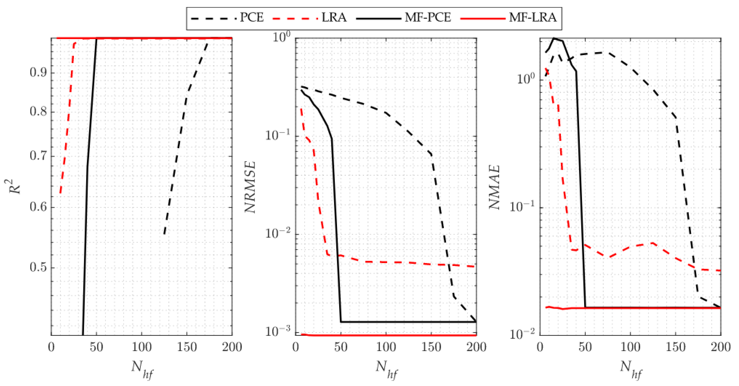
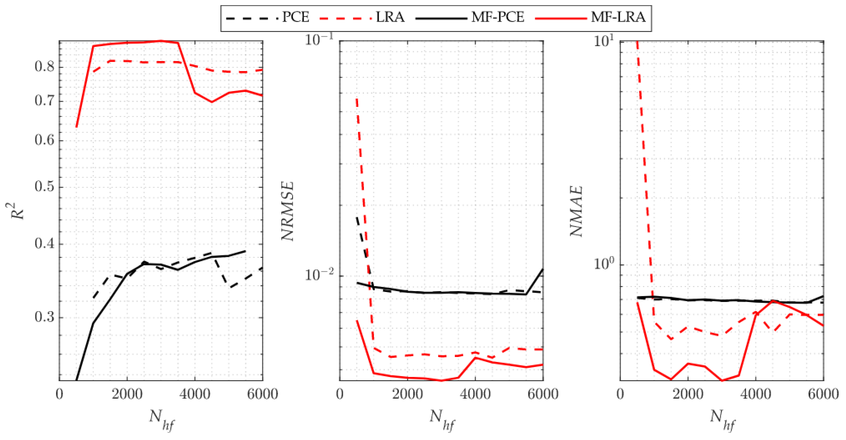
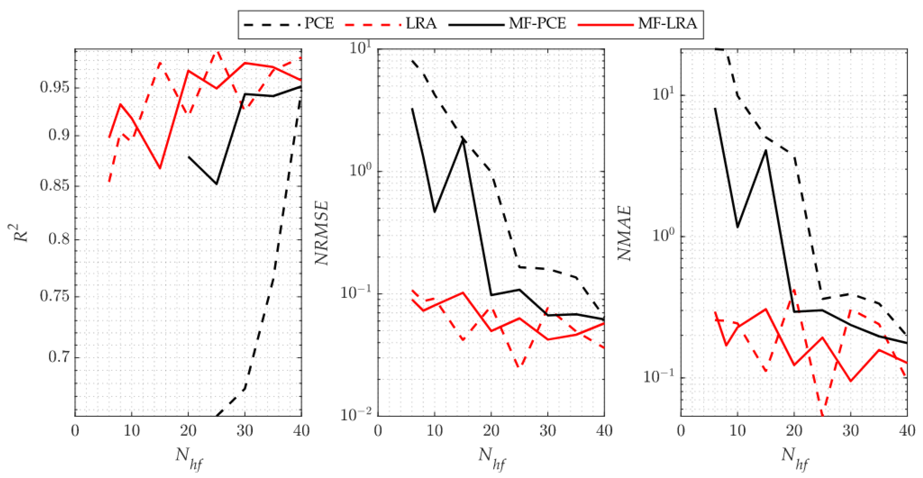
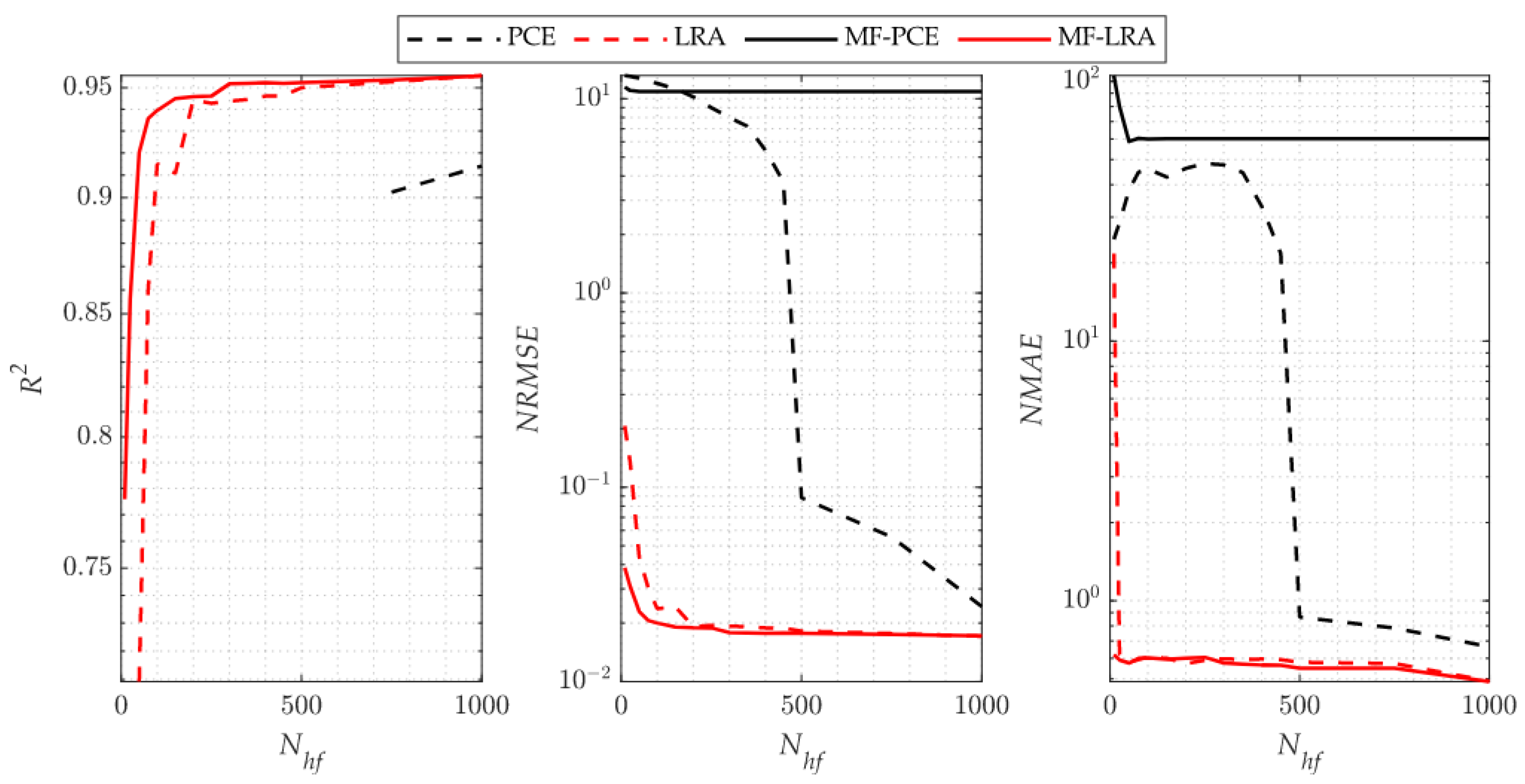
As it is indicated by the accuracy metrics of the single- and multi-fidelity surrogate models for the benchmark problems, an accurate surrogate model can be achieved with a small number of high-fidelity simulations by using the LRA method. When using the PCE method, however, many more high-fidelity simulations are required to set up a single- or multi-fidelity surrogate model with a similar accuracy. The number of high-fidelity simulations required in the single-fidelity PCE method is more than two to three times the number of high-fidelity simulations required in the LRA method for the 4-D Park and 4-D sonic boom uncertainty quantification implementations. However, as the problem dimension increases, it is observed that this ratio is five times in the 8-D Borehole function, and much higher than five times in the 30-D Sobol’-Levitan function and 32-D sonic boom uncertainty quantification problem. The performance difference is attributed to the fact that the LRA method contains fewer unknown coefficients than that of the PCE method due to the univariate polynomials that the LRA method employs. It is observed from the analytical test cases that the single- and multi-fidelity PCE and LRA methods are successful in capturing global features of the response. Since the surrogate modelling methods considered in the present study use orthogonal polynomials that show smooth behaviour in the design space, it can be observed from the $NMAE$ metric that the success of capturing local features is low. These methods are generally preferred in uncertainty and sensitivity analysis due to their ability to deal with the general behaviour of the design space. However, because of their inefficient ability to capture local features, they are generally not preferred for optimisation.

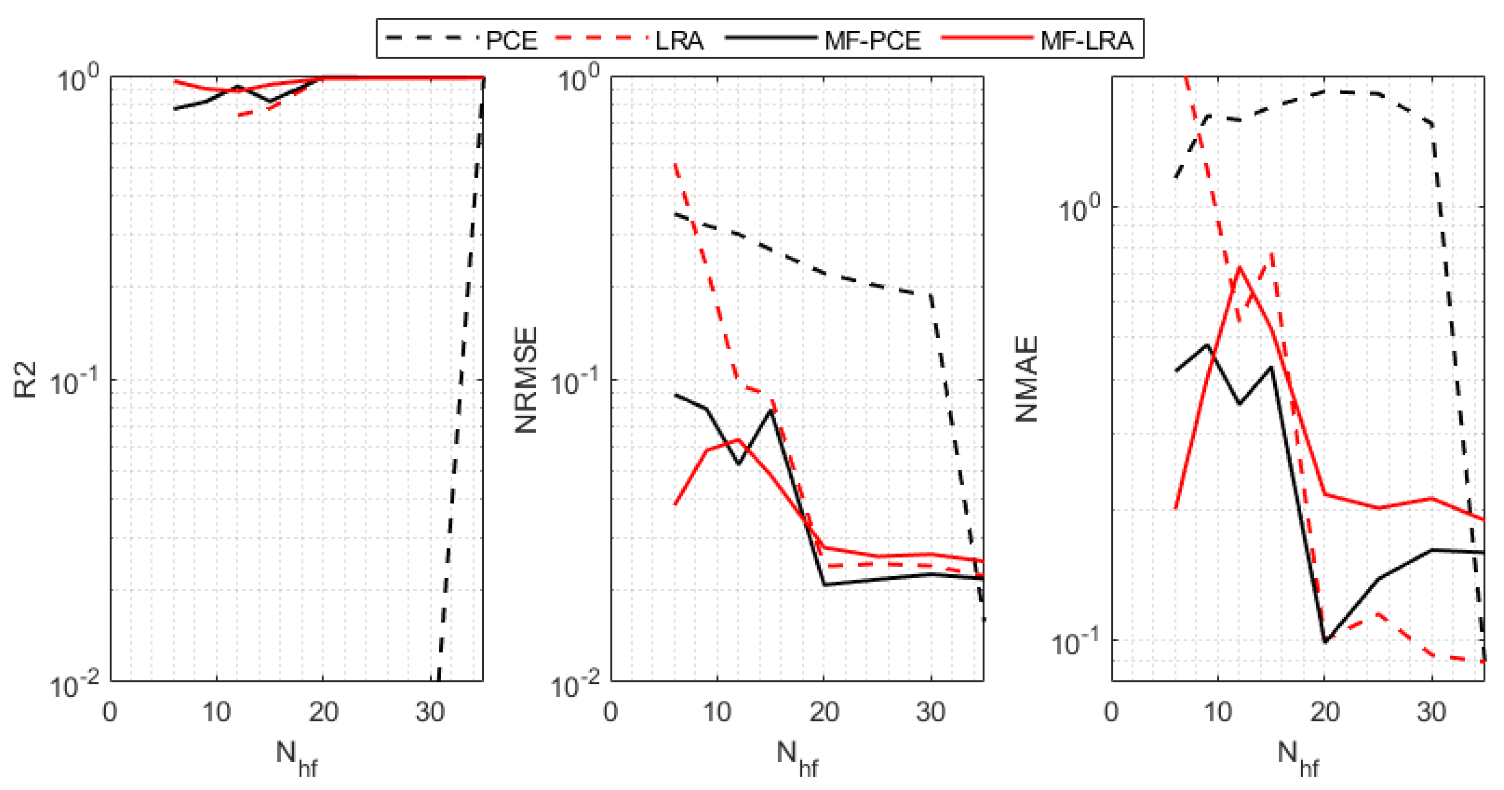
Considering the comparison of the multi-fidelity versions of the methods with the single-fidelity methods, when using the same number of high-fidelity analyses, the multi-fidelity surrogate versions produce more accurate results by making use of low-fidelity model information. When the high-fidelity simulations required to construct a surrogate model with similar accuracy using the LRA and MF-LRA methods are compared, it is observed that the number of high-fidelity simulations required in the LRA method is two to three times the number of simulations needed in the MF-LRA method. Considering the single- and multi-fidelity applications of the PCE method, the number of high-fidelity simulations required in the PCE method for low-dimensional problems is two to three times the number of simulations required by the MF-PCE method. In high-dimensional problems, it is observed that an accurate model cannot be obtained with the multi-fidelity PCE method. In this respect, a more accurate surrogate model can be established with fewer simulations in low- and high-dimensional problems with the LRA method compared to the PCE method. Moreover, with the multi-fidelity version of the LRA method, accurate surrogate models are constructed with only few simulations results. The number of unknowns increases exponentially with the problem dimension in both single- and multi-fidelity PCE methods. Thus, an accurate surrogate model can be established for low-dimensional problems. However, in high-dimensional problems, an accurate surrogate model cannot be established with a low number of simulations. Moreover, the accuracy level of the low-fidelity surrogate model directly affects the ability to model the response of the multi-fidelity surrogate model. The importance of the accuracy level of the low-fidelity model is especially noticeable when the number of high-fidelity analyses are increased in the multi-fidelity surrogate, and it causes the multi-fidelity model to have lower accuracy values than the single-fidelity model, as observed in the Sobol’-Levitan benchmark function and 32-D sonic boom uncertainty quantification problem.

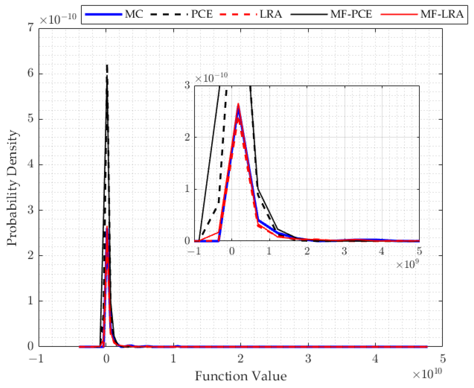
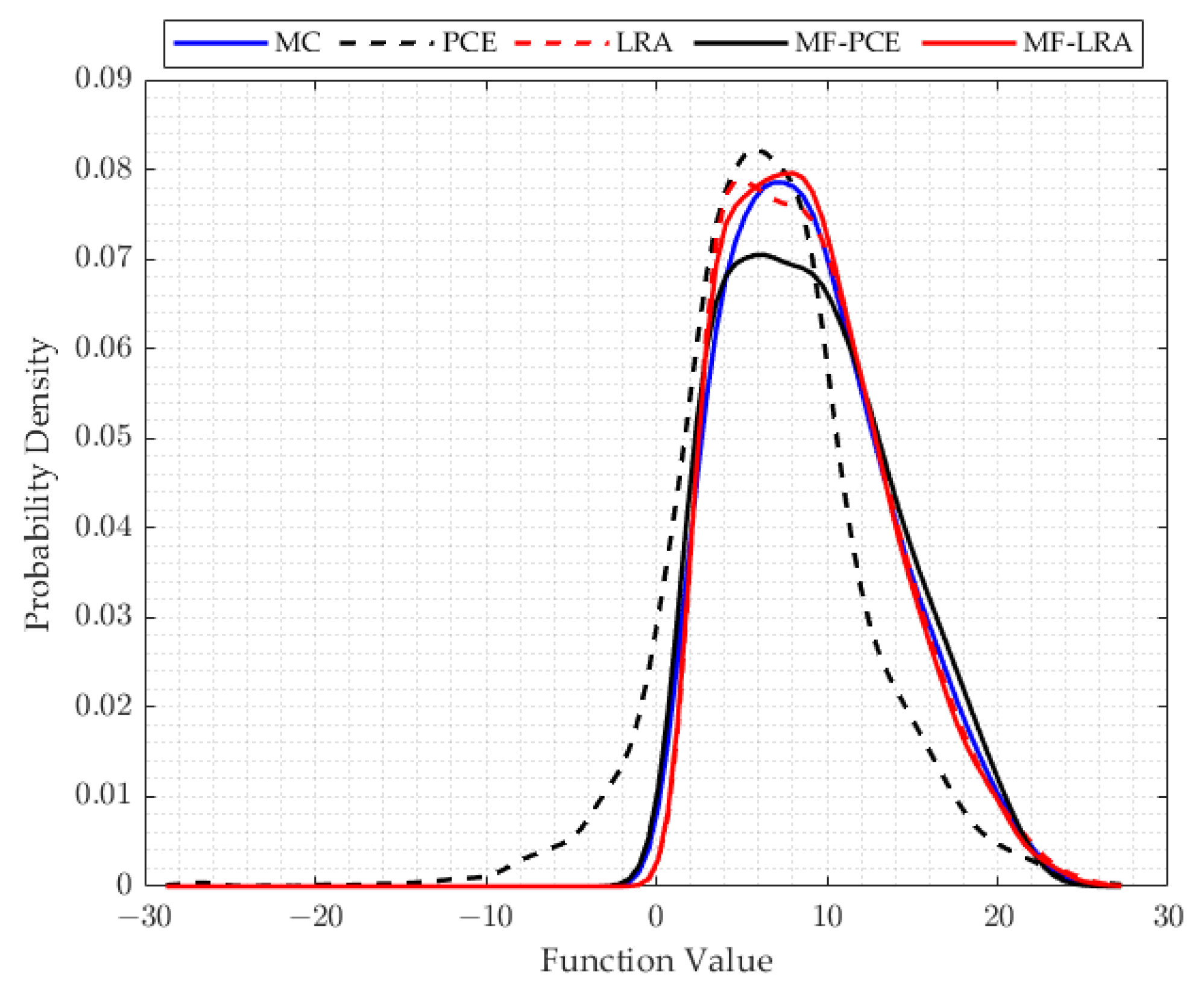
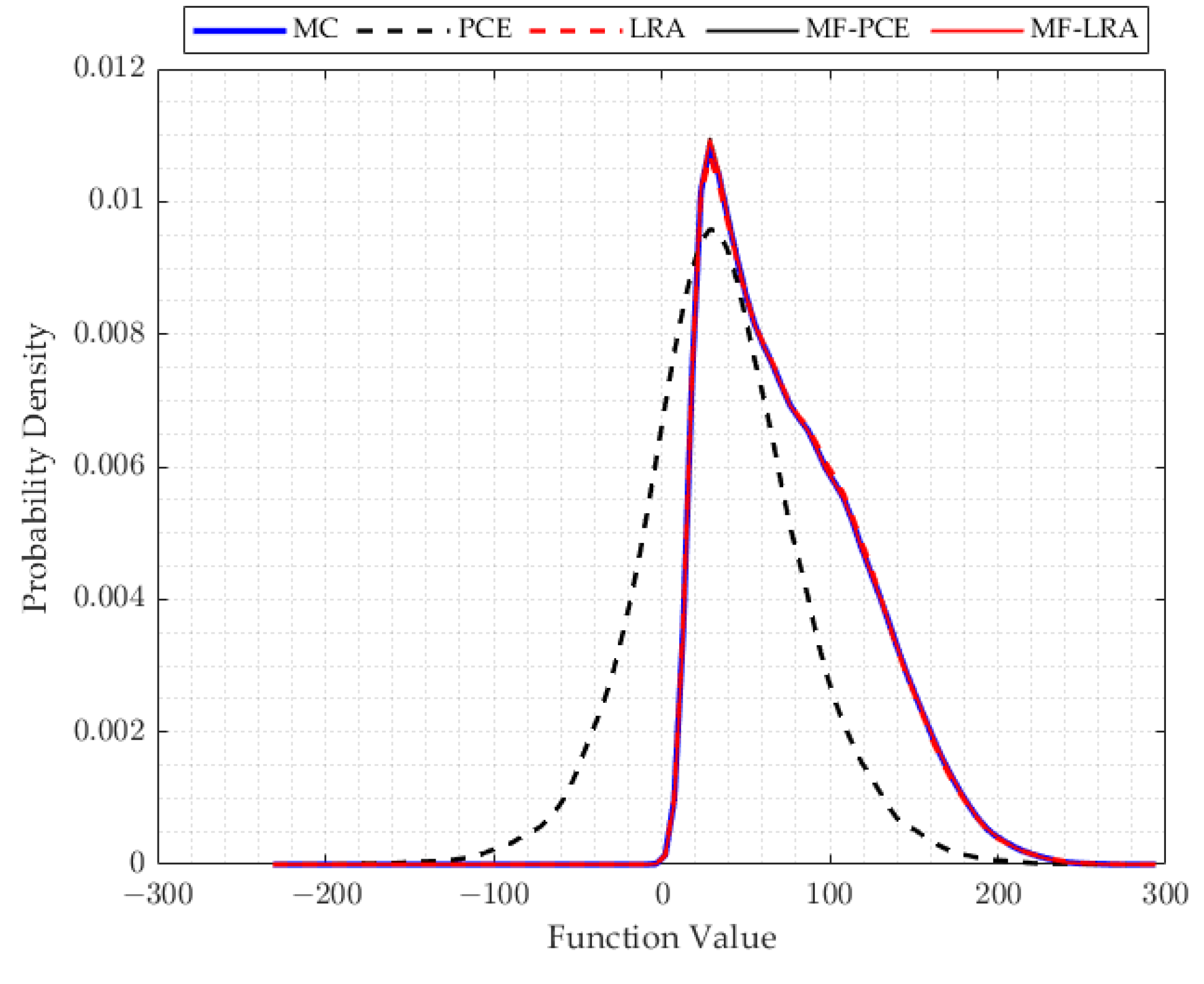
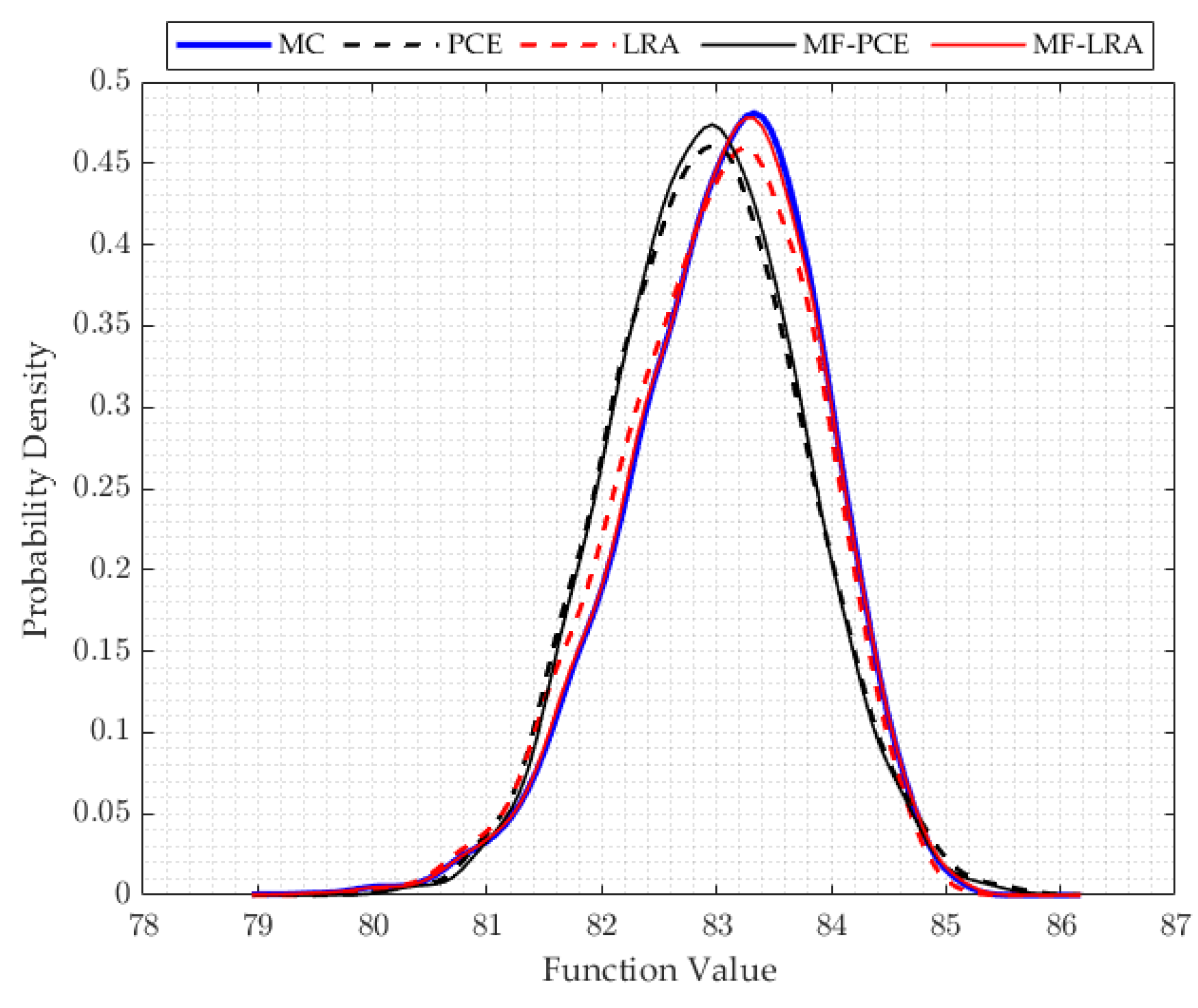
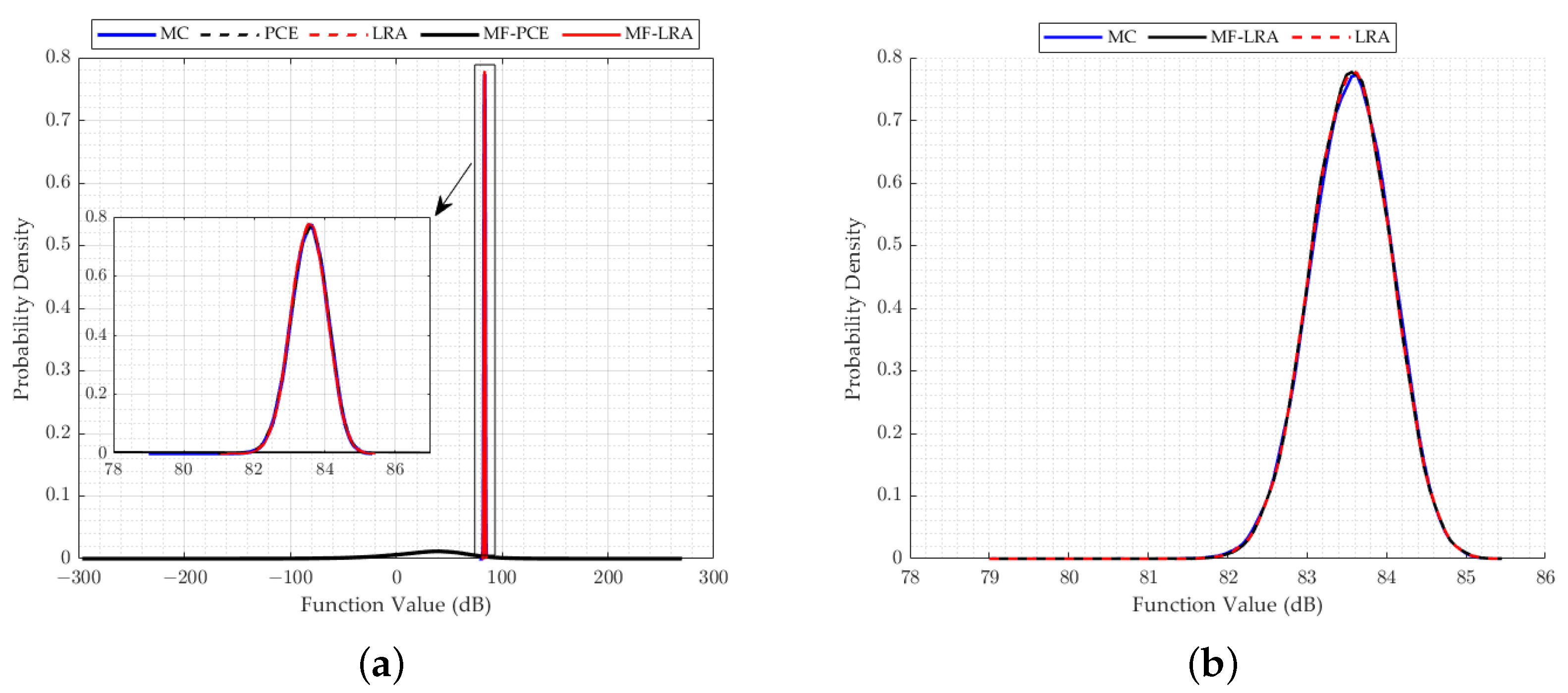
When examining the results of the uncertainty analysis tackled with different methods, it is observed that the PDF results of the LRA method are in good agreement with the MC results, although a small number of the analyses results are used in all applications of the single- and multi-fidelity LRA method. In many applications, when using the same number of results of the analyses, the PDF values obtained by the PCE method produce incompatible results with the MC method. A remarkable point in the results is that the single- and multi-fidelity LRA methods can model the tail region of the PDF very accurately, which has crucial importance in reliability studies. Small probabilities of exceedence used in the reliability analysis can be obtained more accurately by the LRA method which makes the LRA method more advantageous than the PCE method in reliability studies. In addition, the success of the LRA method in modelling the general behaviour of the computational model can be observed from the mean, standard deviation, skewness, and kurtosis values shared in the results of the engineering problem, which can also be observed in PDF functions. While the mean and standard deviation are obtained correctly with the single- and multi-fidelity PCE method, parameter estimates that explain the behaviour of the PDF function such as skewness and kurtosis contain high errors. However, the single- and multi-fidelity LRA method can estimate the mean and standard deviation values, as well as the skewness and kurtosis values, quite accurately.

Despite the outperforming results of the LRA method when compared to another popular polynomial basis approximation, PCE, further investigations are needed for challenging problems to observe the capturing capability for a wide range of benchmarks with diverse mathematical characteristics. Based on the present results, one particular challenge in some implementations may be the ability to capture local behaviours. Therefore, advanced investigations are required to enhance the ability to represent local characteristics. In addition, applications for higher dimensional industrial problems are currently underway.

References

1. Sudret, B.; Marelli, S.; Wiart, J. Surrogate models for uncertainty quantification: An overview. In Proceedings of the 2017 11th European Conference on Antennas and Propagation (EUCAP), Paris, France, 19–24 March 2017; pp. 793–797. [Google Scholar] [CrossRef]
2. Peherstorfer, B.; Willcox, K.; Gunzburger, M. Survey of Multifidelity Methods in Uncertainty Propagation, Inference, and Optimization. SIAM Rev. 2018, 60, 550–591. [Google Scholar] [CrossRef]
3. Konakli, K.; Sudret, B. Reliability analysis of high-dimensional models using low-rank tensor approximations. Probabilistic Eng. Mech. 2016, 46, 18–36. [Google Scholar] [CrossRef] [Green Version]
4. Konakli, K.; Sudret, B. Low-rank tensor approximations for reliability analysis. In Proceedings of the 12th International Conference on Applications of Statistics and Probability in Civil Engineering (ICASP12), Vancouver, BC, Canada, 12–15 July 2015. [Google Scholar]
5. Ehre, M.; Papaiannou, I.; Straub, D. Efficient estimation of variance-based reliability sensitivities in the presence of multi-uncertainty. In Proceedings of the 19th working conference of IFIP Working Group 7.5 on Reliability and Optimization of Structural Systems, Zurich, Switzerland, 26–29 June 2018. [Google Scholar]
6. Doostan, A.; Validi, A.; Iaccarino, G. Non-intrusive low-rank separated approximation of high-dimensional stochastic models. Comput. Methods Appl. Mech. Eng. 2013, 263, 42–55. [Google Scholar] [CrossRef] [Green Version]
7. Validi, A. Low-rank separated representation surrogates of high-dimensional stochastic functions: Application in Bayesian inference. J. Comput. Phys. 2014, 260, 37–53. [Google Scholar] [CrossRef] [Green Version]
8. Chevreuil, M.; Rai, P.; Nouy, A. Sampling based tensor approximation method for uncertainty propagation. Safety, reliability, risk and life-cycle performance of structures and infrastructures. In Proceedings of the 11th International Conference on Structural Safety and Reliability, ICOSSAR 2013, Columbia University, New York, NY, USA, 16–20 June 2013; pp. 3269–3274. [Google Scholar]
9. Konakli, K.; Sudret, B. Uncertainty quantification in high-dimensional spaces with low-rank tensor approximations. In Proceedings of the 1st International Conference on Uncertainty Quantification in Computational Sciences and Engineering (UNCECOMP 2015), Crete Island, Greece, 25–27 May 2015; Institute of Structural Analysis and Antiseismic Research School of Civil Engineering National Technical University of Athens (NTUA): Athens, Greece, 2015. [Google Scholar] [CrossRef] [Green Version]
10. Hadigol, M.; Doostan, A.; Matthies, H.G.; Niekamp, R. Partitioned treatment of uncertainty in coupled domain problems: A separated representation approach. Comput. Methods Appl. Mech. Eng. 2014, 274, 103–124. [Google Scholar] [CrossRef] [Green Version]
11. Konakli, K.; Sudret, B. Global sensitivity analysis using low-rank tensor approximations. Reliab. Eng. Syst. Saf. 2016, 156, 64–83. [Google Scholar] [CrossRef] [Green Version]
12. Konakli, K.; Sudret, B. Polynomial meta-models with canonical low-rank approximations: Numerical insights and comparison to sparse polynomial chaos expansions. J. Comput. Phys. 2016, 321, 1144–1169. [Google Scholar] [CrossRef] [Green Version]
13. Blatman, G.; Sudret, B. Efficient computation of global sensitivity indices using sparse polynomial chaos expansions. Reliab. Eng. Syst. Saf. 2010, 95, 1216–1229. [Google Scholar] [CrossRef]
14. Blatman, G.; Sudret, B. Adaptive sparse polynomial chaos expansion based on least angle regression. J. Comput. Phys. 2011, 230, 2345–2367. [Google Scholar] [CrossRef]
15. Papaioannou, I.; Ehre, M.; Straub, D. PLS-based adaptation for efficient PCE representation in high dimensions. J. Comput. Phys. 2019, 387, 186–204. [Google Scholar] [CrossRef]
16. Son, J.; Du, Y. Modified Dimension Reduction-Based Polynomial Chaos Expansion for Nonstandard Uncertainty Propagation and Its Application in Reliability Analysis. Processes 2021, 9, 1856. [Google Scholar] [CrossRef]
17. Zuhal, L.R.; Faza, G.A.; Palar, P.S.; Liem, R.P. Fast and adaptive reliability analysis via kriging and partial least squares. In Proceedings of the AIAA Scitech 2021 Forum, Virtual Event, Online. 11–15 & 19–21 January 2021; American Institute of Aeronautics and Astronautics: Washington, DC, USA, 2021. [Google Scholar] [CrossRef]
18. Peherstorfer, B.; Beran, P.S.; Willcox, K.E. Multifidelity Monte Carlo estimation for large-scale uncertainty propagation. In Proceedings of the 2018 AIAA Non-Deterministic Approaches Conference, Kissimmee, FL, USA, 8–12 January 2018; American Institute of Aeronautics and Astronautics: Washington, DC, USA, 2018. [Google Scholar] [CrossRef] [Green Version]
19. Quaglino, A.; Pezzuto, S.; Krause, R. High-dimensional and higher-order multifidelity Monte Carlo estimators. J. Comput. Phys. 2019, 388, 300–315. [Google Scholar] [CrossRef] [Green Version]
20. Tekaslan, H.E.; Yildiz, S.; Demiroglu, Y.; Nikbay, M. Implementation of multidisciplinary multi-fidelity uncertainty quantification methods in sonic boom prediction. In AIAA Aviation 2021 Forum; American Institute of Aeronautics and Astronautics: Washington, DC, USA, 2021. [Google Scholar] [CrossRef]
21. Rumpfkeil, M.P.; Beran, P.S. Multifidelity Sparse Polynomial Chaos Surrogate Models Applied to Flutter Databases. AIAA J. 2020, 58, 1292–1303. [Google Scholar] [CrossRef]
22. Xiao, D.; Ferlauto, M.; Song, L.; Li, J. Multi-fidelity sparse polynomial chaos expansion based on Gaussian process regression and least angle regression. J. Phys. Conf. Ser. 2021, 1730, 12091. [Google Scholar] [CrossRef]
23. Ficini, S.; Pellegrini, R.; Odetti, A.; Serani, A.; Iemma, U.; Caccia, M.; Diez, M. Uncertainty quantification of an autonomous surface vehicle by multi-fidelity surrogate models. In Proceedings of the 9th edition of the International Conference on Computational Methods for Coupled Problems in Science and Engineering, CIMNE, Virtual Event, Online. 13–16 June 2021. [Google Scholar] [CrossRef]
24. Rohit, R.J.; Ganguli, R. Co-kriging based multi-fidelity uncertainty quantification of beam vibration using coarse and fine finite element meshes. Int. J. Comput. Methods Eng. Sci. Mech. 2021, 23, 147–168. [Google Scholar] [CrossRef]
25. Piazzola, C.; Tamellini, L.; Pellegrini, R.; Broglia, R.; Serani, A.; Diez, M. Uncertainty quantification of ship resistance via multi-index stochastic collocation and radial basis function surrogates: A comparison. In AIAA Avition 2020 Forum; American Institute of Aeronautics and Astronautics: Washington, DC, USA, 2020. [Google Scholar] [CrossRef]
26. Nagawkar, J.; Leifsson, L. Applications of polynomial chaos-based cokriging to simulation-based analysis and design under uncertainty. In Proceedings of the 46th Design Automation Conference (DAC), San Francisco, CA, USA, 26–31 July 2020; American Society of Mechanical Engineers: New York, NY, USA, 2020; Volume 11. [Google Scholar] [CrossRef]
27. Rumpfkeil, M.P.; Bryson, D.; Beran, P. Multi-Fidelity Sparse Polynomial Chaos and Kriging Surrogate Models Applied to Analytical Benchmark Problems. Algorithms 2022, 15, 101. [Google Scholar] [CrossRef]
28. West, T.; Reuter, B.; Walker, E.; Kleb, W.L.; Park, M.A. Uncertainty quantification and certification prediction of low-boom supersonic aircraft configurations. In Proceedings of the 32nd AIAA Applied Aerodynamics Conference, Atlanta, GA, USA, 16–20 June 2014; American Institute of Aeronautics and Astronautics: Washington, DC, USA, 2014. [Google Scholar] [CrossRef] [Green Version]
29. Phillips, B.D.; West, T.K. Aeroelastic uncertainty quantification of a low-boom aircraft configuration. In Proceedings of the 2018 AIAA Aerospace Sciences Meeting, Kissimmee, FL, USA, 8–12 January 2018; American Institute of Aeronautics and Astronautics: Washington, DC, USA, 2018. [Google Scholar] [CrossRef]
30. Nikbay, M.; Stanford, B.; West, T.K.; Rallabhandi, S.K. Impact of aeroelastic uncertainties on sonic boom signature of a commercial supersonic transport configuration. In Proceedings of the 55th AIAA Aerospace Sciences Meeting, Grapevine, TX, USA, 9–13 January 2017; American Institute of Aeronautics and Astronautics: Washington, DC, USA, 2017. [Google Scholar] [CrossRef]
31. Rallabhandi, S.K.; West, T.K.; Nielsen, E.J. Uncertainty analysis and robust design of low-boom concepts using atmospheric adjoints. In Proceedings of the 33rd AIAA Applied Aerodynamics Conference, Dallas, TX, USA, 22–26 June 2015; American Institute of Aeronautics and Astronautics: Washington, DC, USA, 2015. [Google Scholar] [CrossRef]
32. West, T.K.; Phillips, B.D. Multifidelity Uncertainty Quantification of a Commercial Supersonic Transport. J. Aircr. 2020, 57, 491–500. [Google Scholar] [CrossRef]
33. Marelli, S.; Sudret, B. UQLab: A framework for uncertainty quantification in matlab. In Vulnerability, Uncertainty, and Risk; American Society of Civil Engineers: Liverpool, UK, 2014. [Google Scholar] [CrossRef] [Green Version]
34. Ghanem, R.; Higdon, D.; Owhadi, H. (Eds.) Handbook of Uncertainty Quantification; Springer International Publishing: New York, NY, USA, 2017. [Google Scholar] [CrossRef]
35. Eldred, M.; Burkardt, J. Comparison of non-intrusive polynomial chaos and stochastic collocation methods for uncertainty quantification. In Proceeding of the 47th AIAA Aerospace Sciences Meeting including The New Horizons Forum and Aerospace Exposition, Orlando, FL, USA, 5–8 January 2009; American Institute of Aeronautics and Astronautics: Washington, DC, USA, 2009. [Google Scholar] [CrossRef] [Green Version]
36. Smolyak, S. Quadrature and interpolation formulas for tensor products of certain classes of functions. Sov. Math. Dokl. 1963, 4, 240–243. [Google Scholar]
37. Field, R.V. Numerical methods to estimate the coefficients of the polynomial chaos expansion. In Proceedings of the 15th ASCE Engineering Mechanics Conference, New York, NY, USA, 4 June 2002; Columbia University in the City of New York: Columbia, NY, USA, 2002. [Google Scholar]
38. Maître, O.P.L.; Knio, O.M.; Najm, H.N.; Ghanem, R.G. A Stochastic Projection Method for Fluid Flow. J. Comput. Phys. 2001, 173, 481–511. [Google Scholar] [CrossRef] [Green Version]
39. Hosder, S.; Walters, R.; Balch, M. Efficient sampling for non-intrusive polynomial chaos applications with multiple uncertain input variables. In Proceedings of the 48th AIAA/ASME/ASCE/AHS/ASC Structures, Structural Dynamics, and Materials Conference, Honolulu, HI, USA, 23–26 April 2007; American Institute of Aeronautics and Astronautics: Washington, DC, USA, 2007. [Google Scholar] [CrossRef]
40. Konakli, K.; Mylonas, C.; Marelli, S.; Sudret, B. UQLab User Manual—Canonical Low-Rank Approximations; Technical Report, Report UQLab-V2.0-108; Chair of Risk, Safety and Uncertainty Quantification: Zurich, Switzerland, 2022. [Google Scholar]
41. Chevreuil, M.; Lebrun, R.; Nouy, A.; Rai, P. A Least-Squares Method for Sparse Low Rank Approximation of Multivariate Functions. SIAM/ASA J. Uncertain. Quantif. 2015, 3, 897–921. [Google Scholar] [CrossRef]
42. Ng, L.W.T.; Eldred, M. Multifidelity uncertainty quantification using non-intrusive polynomial chaos and stochastic collocation. In Proceedings of the 53rd AIAA/ASME/ASCE/AHS/ASC Structures, Structural Dynamics and Materials Conference, Honolulu, HI, USA, 23–26 April 2012; American Institute of Aeronautics and Astronautics: Washington, DC, USA, 2012. [Google Scholar] [CrossRef] [Green Version]
43. Morris, M.D.; Mitchell, T.J. Exploratory designs for computational experiments. J. Stat. Plan. Inference 1995, 43, 381–402. [Google Scholar] [CrossRef] [Green Version]
44. McKay, M.D.; Beckman, R.J.; Conover, W.J. Comparison of Three Methods for Selecting Values of Input Variables in the Analysis of Output from a Computer Code. Technometrics 1979, 21, 239–245. [Google Scholar] [CrossRef]
45. Rajabi, M.M.; Ataie-Ashtiani, B.; Janssen, H. Efficiency enhancement of optimized Latin hypercube sampling strategies: Application to Monte Carlo uncertainty analysis and meta-modeling. Adv. Water Resour. 2015, 76, 127–139. [Google Scholar] [CrossRef] [Green Version]
46. Kocis, L.; Whiten, W.J. Computational investigations of low-discrepancy sequences. ACM Trans. Math. Softw. 1997, 23, 266–294. [Google Scholar] [CrossRef]
47. Yildiz, S.; Cakmak, E.; Kara, E.; Nikbay, M. Uncertainty quantification of aeroelastic systems using active learning gaussian process. In Proceedings of the International Conference on Multidisciplinary Design Optimization of Aerospace Systems (AEROBEST 2021), Virtual Event, Online, 21–23 July 2021; Marta, A.C., Suleman, A., Eds.; IDMEC, Instituto Superior Técnico, Universidade de Lisboa: Lisboa, Portugal, 2021; pp. 1–758. [Google Scholar]
48. Xiong, S.; Qian, P.Z.G.; Wu, C.F.J. Sequential Design and Analysis of High-Accuracy and Low-Accuracy Computer Codes. Technometrics 2012, 55, 37–46. [Google Scholar] [CrossRef]
49. Sobol’, I.; Levitan, Y. On the use of variance reducing multipliers in Monte Carlo computations of a global sensitivity index. Comput. Phys. Commun. 1999, 117, 52–61. [Google Scholar] [CrossRef]
50. Rallabhandi, S.K. Advanced Sonic Boom Prediction Using the Augmented Burgers Equation. J. Aircr. 2011, 48, 1245–1253. [Google Scholar] [CrossRef]
51. Demiroglu, Y.; Yildiz, S.; Nikbay, M. Multi-fidelity sonic boom minimization of a supersonic aircraft by parametric wing shape design. In AIAA Scitech 2021 Forum; American Institute of Aeronautics and Astronautics: Washington, DC, USA, 2021. [Google Scholar] [CrossRef]
52. Carmichael, R.; Erickson, L. PAN AIR—A higher order panel method for predicting subsonic or supersonic linear potential flows about arbitrary configurations. In Proceedings of the 14th Fluid and Plasma Dynamics Conference. American Institute of Aeronautics and Astronautics, Palo Alto, CA, USA, 23–25 June 1981. [Google Scholar] [CrossRef]
53. Economon, T.D.; Palacios, F.; Copeland, S.R.; Lukaczyk, T.W.; Alonso, J.J. SU2: An Open-Source Suite for Multiphysics Simulation and Design. AIAA J. 2016, 54, 828–846. [Google Scholar] [CrossRef]
54. Park, M.A.; Nemec, M. Nearfield Summary and Statistical Analysis of the Second AIAA Sonic Boom Prediction Workshop. J. Aircr. 2019, 56, 851–875. [Google Scholar] [CrossRef]
55. Carpenter, F.L.; Cizmas, P.; Bolander, C.R.; Giblette, T.N.; Hunsaker, D.F. A multi-fidelity prediction of aerodynamic and sonic boom characteristics of the JAXA wing body. In AIAA Aviation 2019 Forum; American Institute of Aeronautics and Astronautics: Washington, DC, USA, 2019. [Google Scholar] [CrossRef]
Figure 1. Comparing number of unknown coefficients between the PCE and LRA methods for high dimensional problems.
Algorithms 15 00250 g001
Figure 2. Comparison of sampling methods [47].
Algorithms 15 00250 g002
Figure 3. Surrogate model error metrics for Park (1991) function ( N l f = 35 ).
Algorithms 15 00250 g003
Figure 4. Comparison of probability density function ( N h f = 20 , N l f = 35 ).
Algorithms 15 00250 g004
Figure 5. Surrogate model error metrics for Borehole function ( N l f = 200 ).
Algorithms 15 00250 g005
Figure 6. Comparison of probability density function ( N h f = 50 , N l f = 200 ).
Algorithms 15 00250 g006
Figure 7. Surrogate model error metrics for Sobol’-Levitan function ( N l f = 10,000).
Algorithms 15 00250 g007
Figure 8. Comparison of probability density function ( N h f = 2500 , N l f = 10,000).
Algorithms 15 00250 g008
Figure 9. Aeroacoustic propagation in sonic boom prediction. Reproduced with permission from Ref. [51].
Algorithms 15 00250 g009
Figure 10. The JAXA Wing-Body geometry.
Algorithms 15 00250 g010
Figure 11. Pressure coefficient distribution comparison (a) on the upper surface (b) on the lower surface.
Algorithms 15 00250 g011
Figure 12. Pressure signature comparison: (a) Near-field pressure signature (b); ground signature for JWB.
Algorithms 15 00250 g012
Figure 13. Surrogate model error metrics for sonic boom problem 1 ( N l f = 70 ).
Algorithms 15 00250 g013
Figure 14. Comparison of probability density function ( N l f = 70 , N h f = 40 ).
Algorithms 15 00250 g014
Figure 15. Surrogate model error metrics for sonic boom problem 2 ( N l f = 1000 ).
Algorithms 15 00250 g015
Figure 16. Comparison of probability density function (a) Results of all surrogate models (b) Results of LRA and MF-LRA ( N h f = 500 , N l f = 1000 ).
Algorithms 15 00250 g016