
Optimizing Finite-Difference Operator in Seismic Wave Numerical Modeling


Abstract
:1. Introduction
2. Methods
2.1. Finite-Difference Method
2.2. Modeling
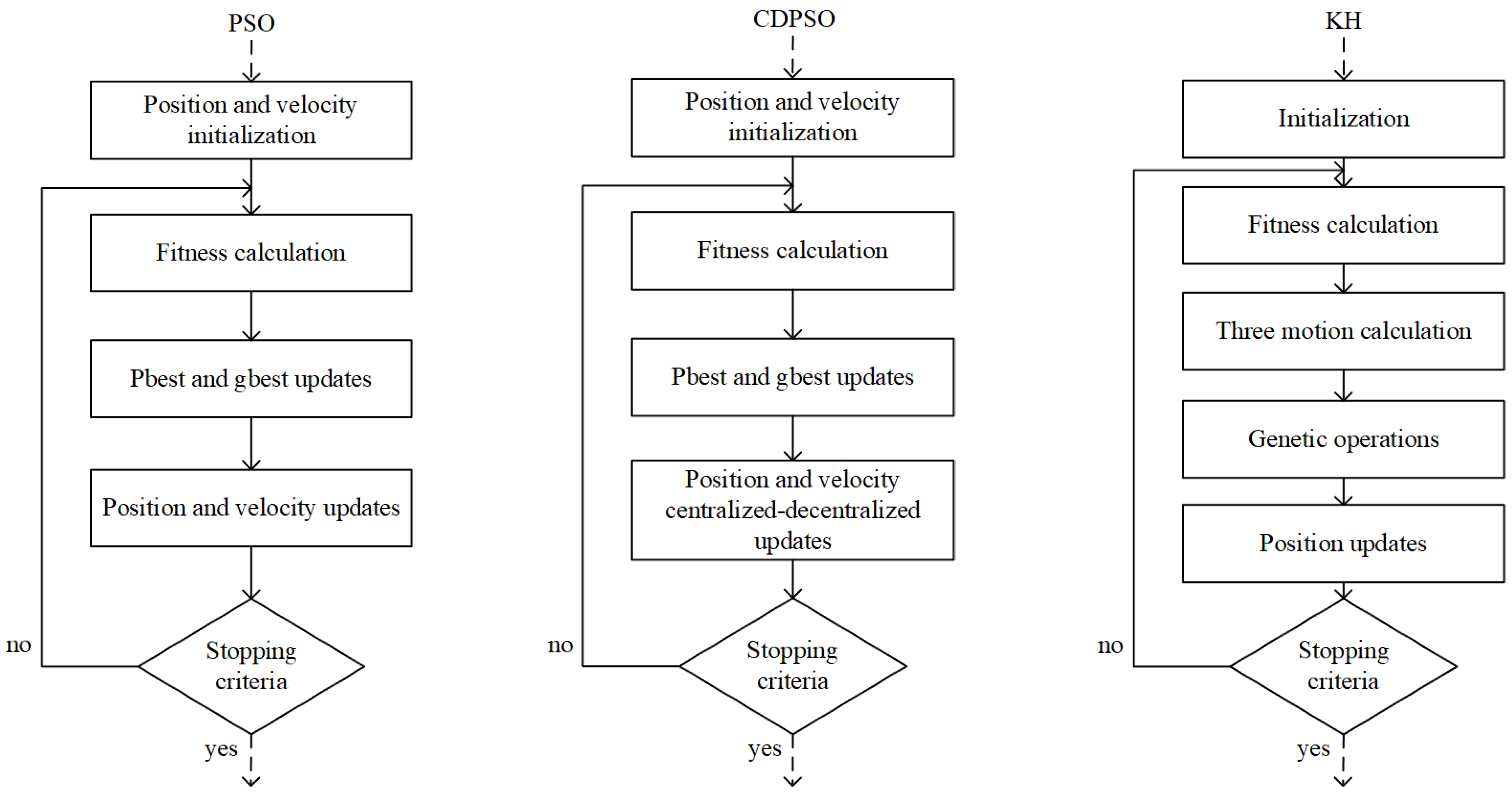
2.3. Three Optimization Algorithms
2.3.1. Particle Swarm Optimization
2.3.2. Center–Decenter PSO
2.3.3. Krill Herd Algorithm
3. Numerical Simulation
3.1. Simulation Setup
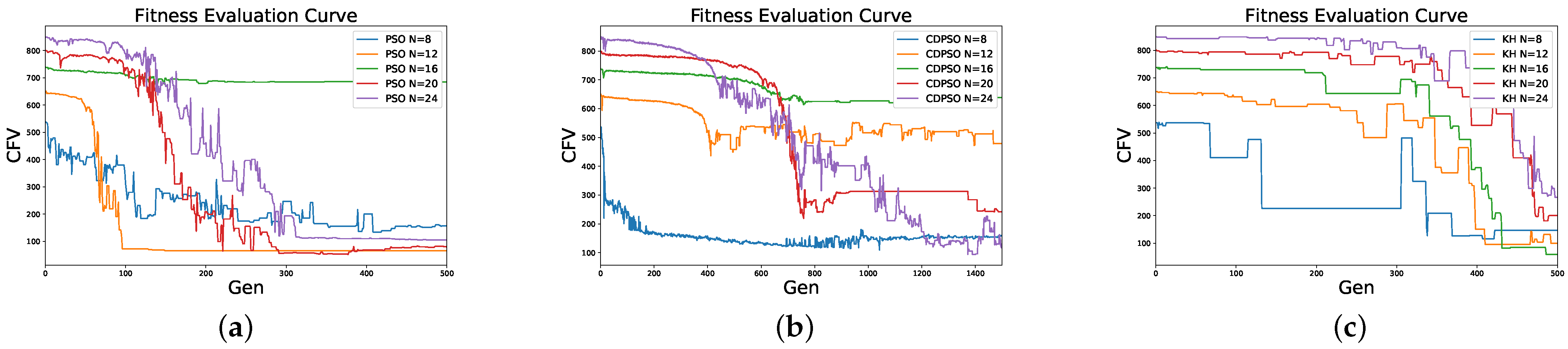
3.2. Coefficients Convergence
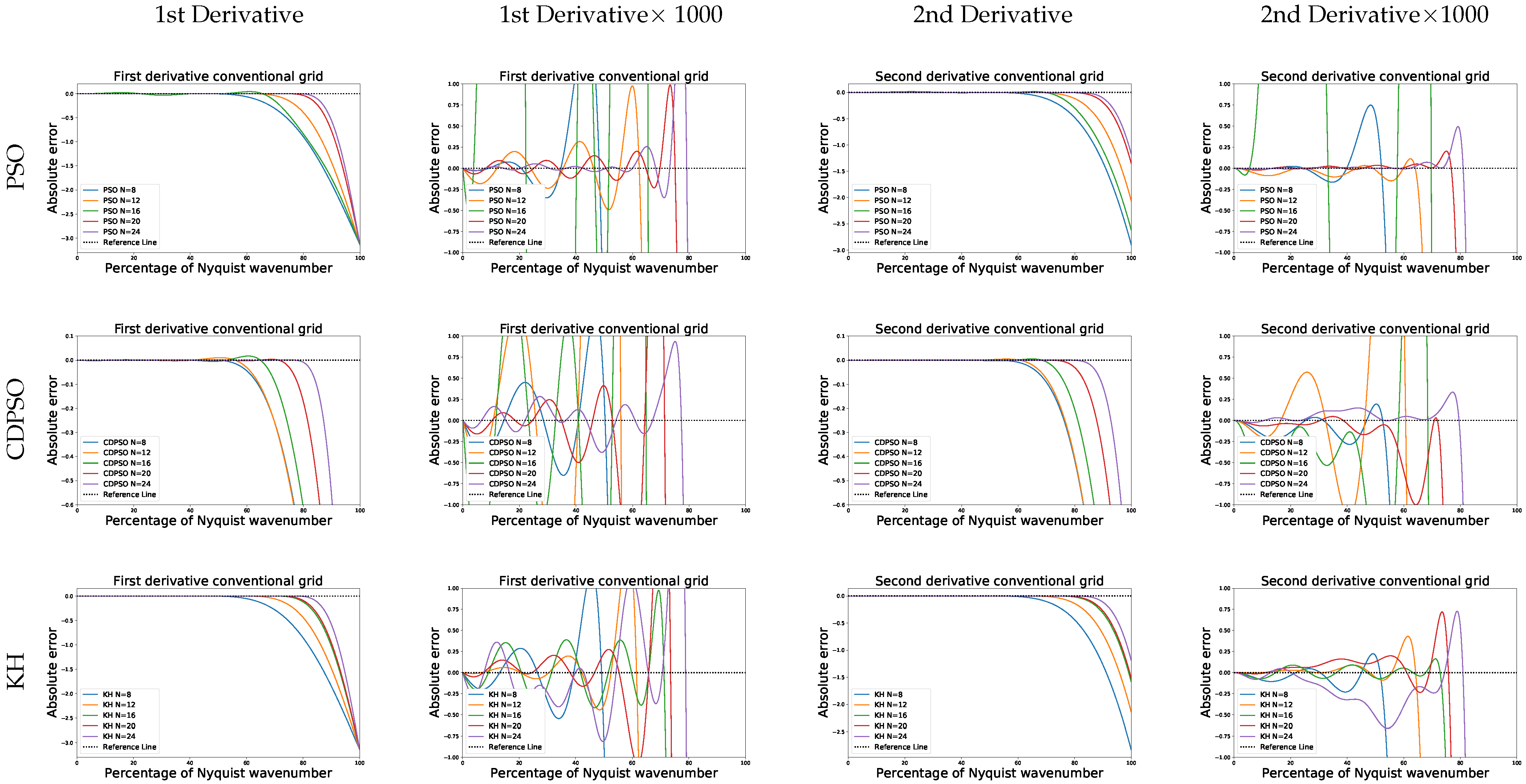
3.3. Stability
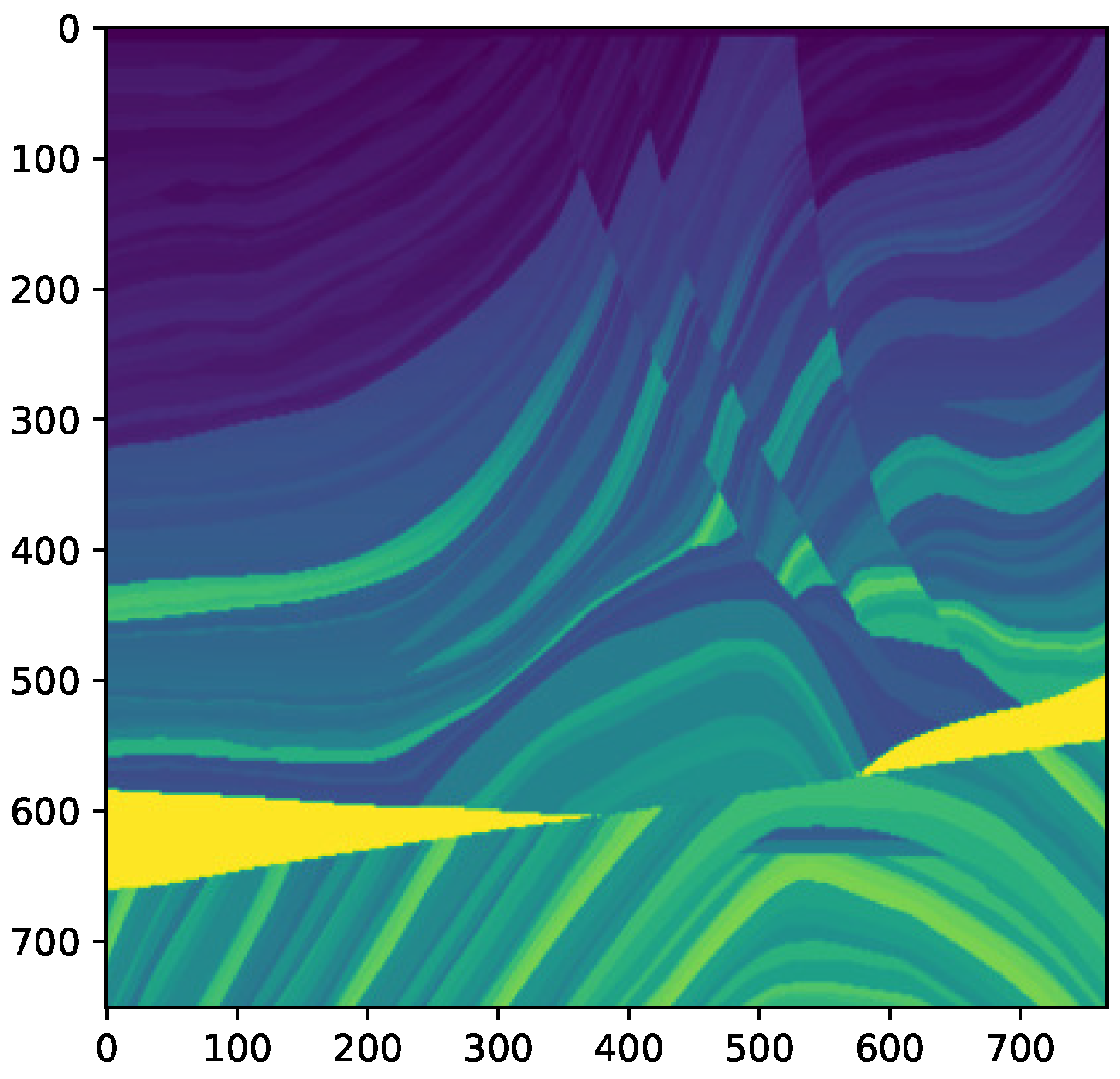
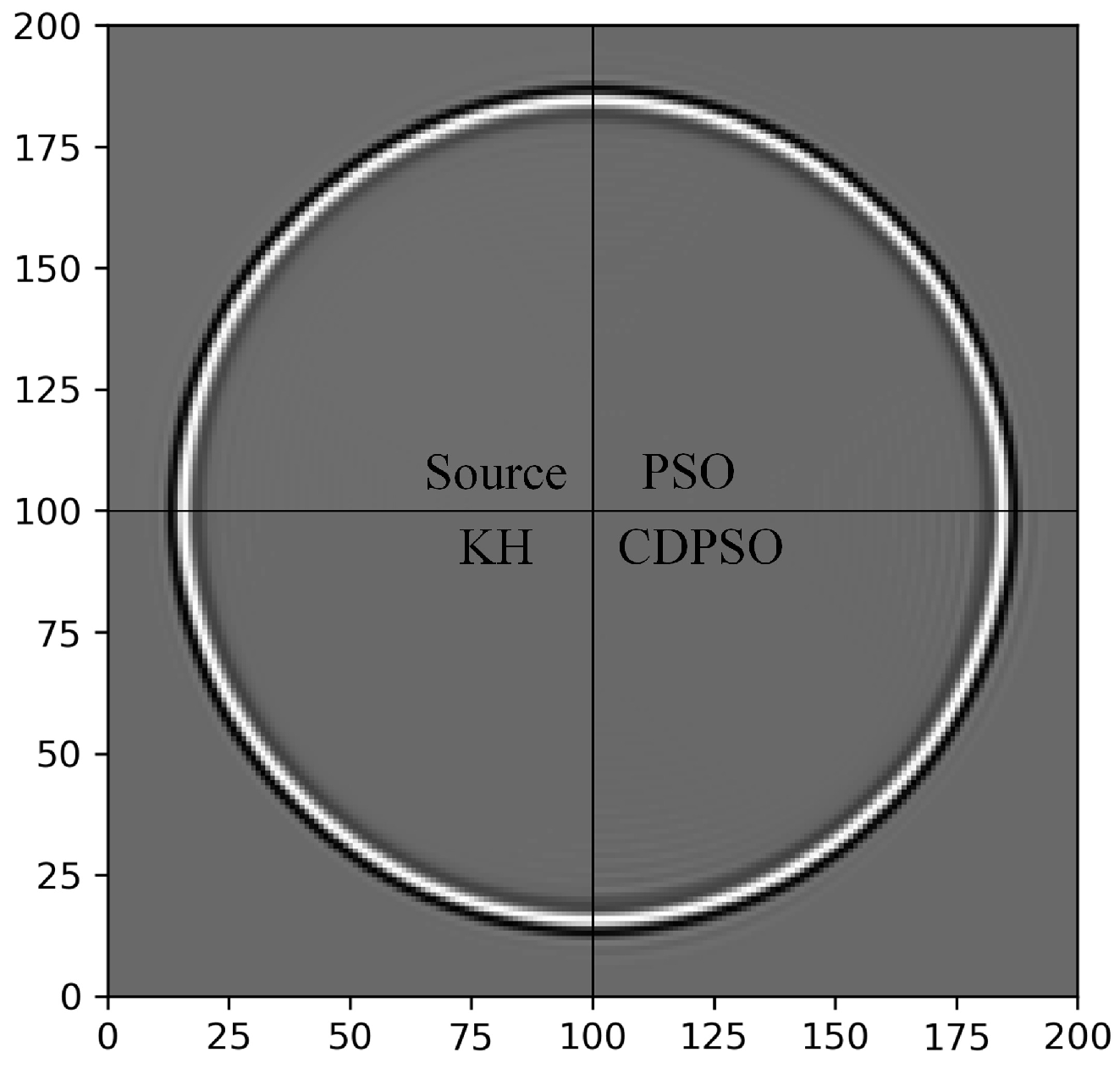
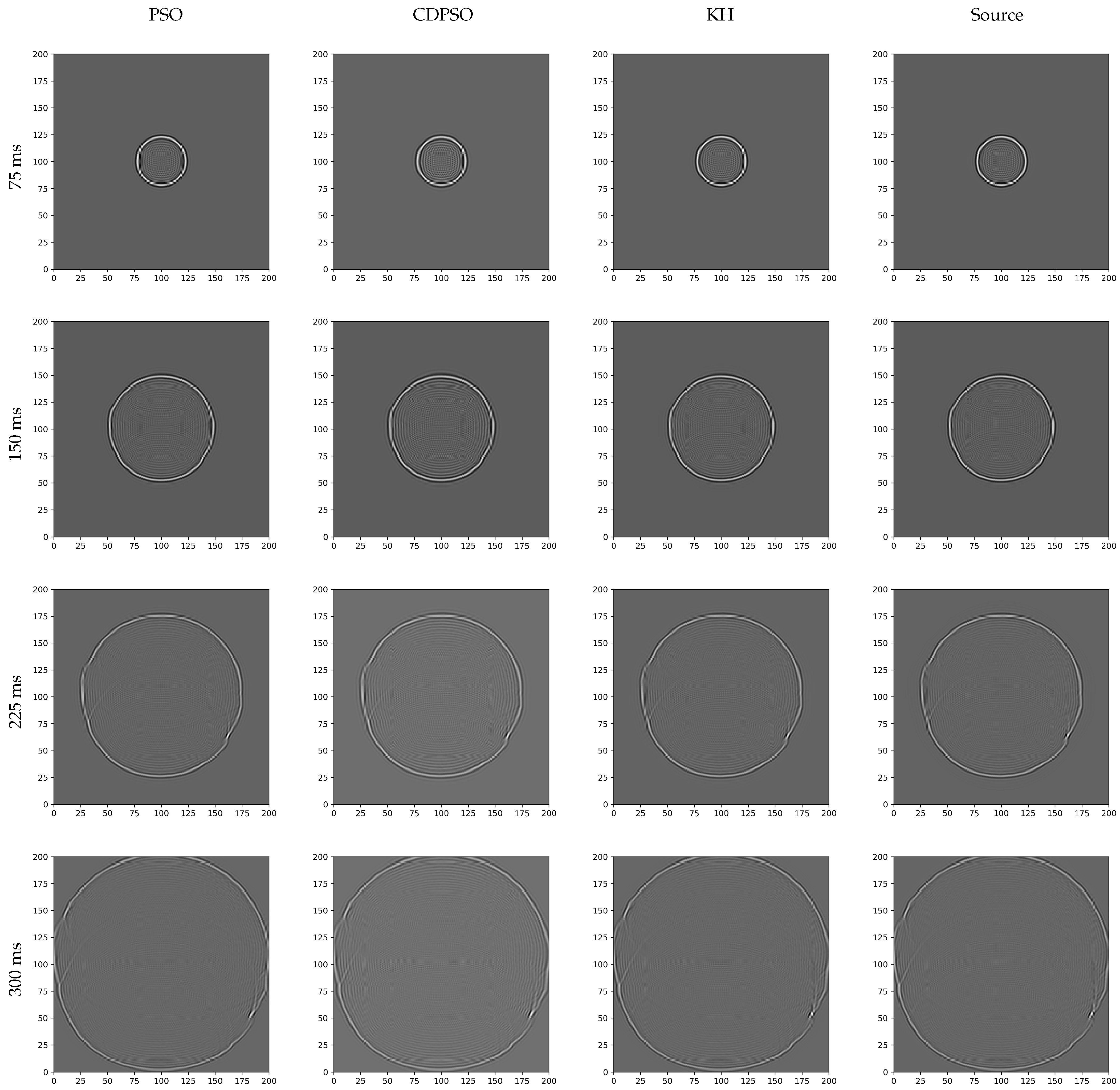
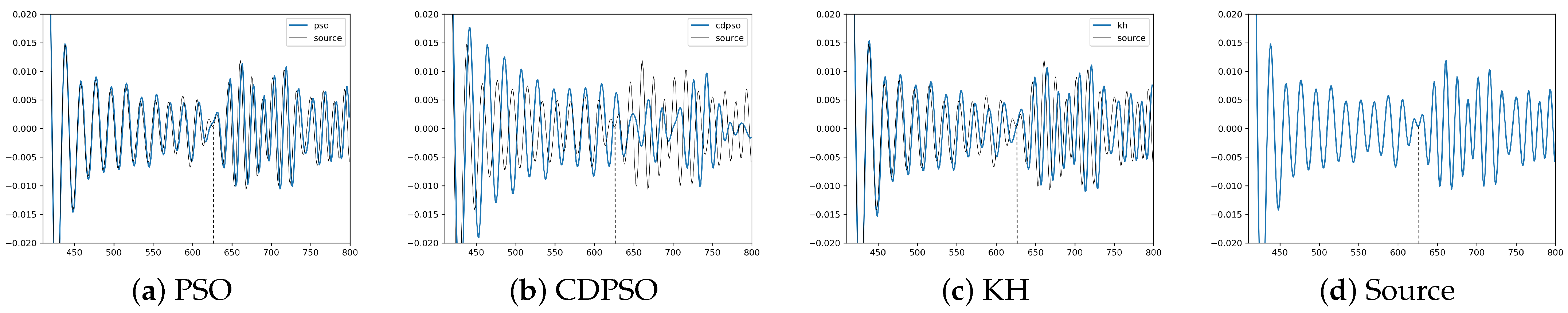
3.4. Model Test
4. Conclusions
Author Contributions
Funding
Data Availability Statement
Conflicts of Interest
Appendix A. FD Operator
Appendix A.1. The First and Second Derivatives of f
Appendix A.2. The FD Operator through Taylor’s Expansion
Appendix A.3. Fourier Transform
References
- Favorskaya, A.; Petrov, I.; Golubev, V.; Khokhlov, N. Numerical simulation of earthquakes impact on facilities by grid-characteristic method. Matem. Mod. 2017, 112, 1206–1215. [Google Scholar] [CrossRef]
- Sarchi, L.; Varum, H.; Monteiro, R.; Silveira, D. Seismic behavior of two Portuguese adobe buildings: Part II—Numerical modeling and fragility assessment. Int. J. Archit. Herit. 2018, 12, 936–950. [Google Scholar] [CrossRef]
- Chen, X.; Fu, J.; Xue, F.; Wang, X. Comparative Numerical Research on the Seismic Behavior of RC Frames Using Normal and High-Strength Reinforcement. Int. J. Civ. Eng. 2017, 15, 531–547. [Google Scholar] [CrossRef]
- Chen, J.; Tong, S.; Han, T.; Song, H.; Pinheiro, L.; Xu, H.; Azevedo, L.; Duan, M.; Liu, B. Modelling and detection of submarine bubble plumes using seismic oceanography. J. Mar. Syst. 2020, 209, 103375. [Google Scholar] [CrossRef]
- Lu, Z.; Zhang, Z.; Gu, J. Modeling of low-frequency seismic waves in a shallow sea using the staggered grid difference method. Chin. J. Oceanol. Limnol. 2017, 35, 1010–1017. [Google Scholar] [CrossRef]
- Yao, G.; Wu, D.; Debens, H.A. Adaptive finite difference for seismic wavefield modelling in acoustic media. Sci. Rep. 2016, 6, 30302. [Google Scholar] [CrossRef]
- Alterman, Z.; Karal, F. Propagation of elastic waves in layered media by Finite Difference methods. Bull. Seismol. Soc. Am. 1968, 58, 367–398. [Google Scholar]
- Lysmer, J.; Drake, L.A. A Finite Element Method for Seismology. Methods Comput. Phys. Adv. Res. Appl. 1972, 11, 181–216. [Google Scholar]
- SU, B.; Li, H.; Liu, S.; Yang, D. Modified symplectic scheme with finite element method for seismic wavefield modeling. Chin. J. Geophys. 2019, 62, 1440–1452. [Google Scholar]
- Jiang, X.; Adeli, H. Pseudospectra, MUSIC, and dynamic wavelet neural network for damage detection of highrise buildings. Int. J. Numer. Methods Eng. 2007, 71, 606–629. [Google Scholar] [CrossRef]
- Kalyani, V.K.; Sinha, A.; Pallavika; Chakraborty, S.K.; Mahanti, N.C. Finite difference modeling of seismic wave propagation in monoclinic media. Acta Geophys. 2008, 56, 1074–1089. [Google Scholar] [CrossRef]
- Fornberg, B. The pseudospectral method; comparisons with finite differences for the elastic wave equation. Geophysics 1987, 52, 483–501. [Google Scholar] [CrossRef]
- Zhou, B.; Greenhalgh, S. Seismic scalar wave equation modeling by a convolutional differentiator. Bull. Seismol. Soc. Am. 1992, 82, 289–303. [Google Scholar]
- Igel, H.; Mora, P.; Riollet, B. Anisotropic wave propagation through finite-difference grids. Geophysics 1995, 60, 1203–1216. [Google Scholar] [CrossRef]
- Hicks, G.J. Arbitrary source and receiver positioning in finite-difference schemes using Kaiser windowed sinc functions. Geophysics 2002, 67, 156–165. [Google Scholar] [CrossRef]
- Wang, Z.; Liu, H.; Tang, X.D.; Wang, Y. Optimized Finite-Difference Operators Based on Chebyshev Auto-Convolution Combined Window Function. Chin. J. Geophys. 2015, 58, 628–642. [Google Scholar]
- Zheng, W.Q.; Meng, X.H.; Liu, J.H.; Wang, J.H. High precision elastic wave equation forward modeling based on cosine modulated Chebyshev window function. Chin. J. Geophys. 2016, 59, 2650–2662. [Google Scholar]
- Wang, J.; Hong, L. Stable optimization of finite-difference operators for seismic wave modeling. Stud. Geophys. Geod. 2020, 64, 452. [Google Scholar] [CrossRef]
- Zhang, J.H.; Yao, Z.X. Optimized finite-difference operator for broadband seismic wave modeling. Geophysics 2012, 78, A13–A18. [Google Scholar] [CrossRef] [Green Version]
- Wang, Z.Y.; Bai, W.L.; Liu, H. An optimized finite-difference scheme based on the improved PSO algorithm for wave propagation. In SEG Technical Program Expanded Abstracts 2019; Society of Exploration Geophysicists: Houston, TX, USA, 2019. [Google Scholar]
- Ren, Y.J.; Huang, J.P.; Peng, Y.; Liu, M.L.; Chao, C.; Yang, M.W. Optimized staggered-grid finite-difference operators using window functions. Appl. Geophys. 2018, 15, 253–260. [Google Scholar] [CrossRef]
- Chu, C.; Stoffa, P. Determination of finite-difference weights using scaled binomial windows. Geophysics 2012, 77, W17–W26. [Google Scholar] [CrossRef]
- Bai, W.; Wang, Z.; Liu, H.; Yu, D.; Chen, C.; Zhu, M. Optimisation of the finite-difference scheme based on an improved PSO algorithm for elastic modelling. Explor. Geophys. 2020, 52, 419–430. [Google Scholar] [CrossRef]
- Thongyoy, W.; Boonyasiriwat, C. Least-Squares Finite Difference Operator. 2015. Available online: https://mcsc.sc.mahidol.ac.th/publications/reports/2015/2015-01.pdf (accessed on 8 April 2022).
- Lailly, P.; Rocca, F.; Versteeg, R. The Marmousi experience: Synthesis. In Proceedings of the EAEG Workshop-Practical Aspects of Seismic Data Inversion, Copenhagen, Denmark, 28 May–1 June 1990. [Google Scholar] [CrossRef]
- Kennedy, J.; Eberhart, R. Particle swarm optimization. In Proceedings of the ICNN’95—International Conference on Neural Networks, Perth, Australia, 27 November–1 December 1995; Volume 4, pp. 1942–1948. [Google Scholar]
- Eberhart, R.; Kennedy, J. A new optimizer using particle swarm theory. In Proceedings of the Sixth International Symposium on Micro Machine and Human Science, MHS’95, Nagoya, Japan, 4–6 October 1995; pp. 39–43. [Google Scholar]
- Gandomi, A.H.; Alavi, A.H. Krill herd: A new bio-inspired optimization algorithm. Commun. Nonlinear Sci. Numer. Simul. 2012, 17, 4831–4845. [Google Scholar] [CrossRef]


| Symbol | Meaning |
|---|---|
| sampling interval | |
| sampling point | |
| N | order |
| signal | |
| sample of | |
| window function | |
| , | truncation errors of the first and second derivative |
| , | FD coefficients of the first and second derivative |
| error limitation | |
| wavenumber | |
| max wavenumber | |
| cutoff wavenumber |
| 0.849367818 | 0.920977162 | 0.877587089 | 0.965287713 | 0.973893871 | |
| −0.25408939 | −0.3577484 | −0.288519626 | −0.433682998 | −0.449521466 | |
| 0.065186786 | 0.153433266 | 0.079759689 | 0.24111591 | 0.261752507 | |
| −0.009222605 | −0.058927291 | 0 | −0.139204287 | −0.161705926 | |
| 0.017640291 | 0 | 0.078452231 | 0.1 | ||
| −0.003169356 | −0.006035286 | −0.041571492 | −0.06002697 | ||
| 0.013566605 | 0.020009949 | 0.034157136 | |||
| −0.013048505 | −0.008365952 | −0.017995371 | |||
| 0.002801649 | 0.008513142 | ||||
| −0.00060467 | −0.003450766 | ||||
| 0.001103313 | |||||
| −0.000224999 |
| 0.860321205 | 0.86109756 | 0.897879165 | 0.945915193 | 0.973635331 | |
| −0.26835603 | −0.266916073 | −0.319377704 | −0.399220361 | −0.449084566 | |
| 0.074799005 | 0.070567648 | 0.112048086 | 0.198575497 | 0.261348878 | |
| −0.012312666 | −0.008783105 | −0.026268214 | −0.096211902 | −0.161442267 | |
| 7.08 × | 0.000414949 | 0.041381255 | 0.099999422 | ||
| −0.000970876 | −0.1.99 × | −0.014264206 | −0.06040469 | ||
| 0.002950187 | 0.003122273 | 0.034861698 | |||
| −0.002579216 | −0.000113252 | −0.018844889 | |||
| 0.5.24 × | 0.009398521 | ||||
| −0.000148269 | −0.004199285 | ||||
| 0.001607051 | |||||
| −0.000460175 |
| 0.85637065 | 0.91565981 | 0.953061594 | 0.956976127 | 0.973409618 | |
| −0.263266133 | −0.349228563 | −0.411757109 | −0.418632603 | −0.448750956 | |
| 0.071389175 | 0.144791061 | 0.213788114 | 0.222144041 | 0.260615495 | |
| −0.011184471 | −0.052565668 | −0.111261167 | −0.119424376 | −0.160355857 | |
| 0.014337537 | 0.053990931 | 0.060681453 | 0.098818855 | ||
| −0.002178404 | −0.023007227 | −0.027737712 | −0.059118172 | ||
| 0.007967749 | 0.010823998 | 0.033637319 | |||
| −0.00182424 | −0.003382806 | −0.01775192 | |||
| 0.000823068 | 0.008525232 | ||||
| −0.000185621 | −0.003794 | ||||
| 0.00150656 | |||||
| −0.000518958 |
| Source | −3.138521049 | 1.854196962 | −0.368305121 | 0.110295386 | −0.034584857 | 0.009637126 | −0.001978972 |
| PSO | −3.126061573 | 1.841954323 | −0.3577484 | 0.102288844 | −0.029463646 | 0.007056116 | −0.001056452 |
| CDPSO | −2.995218501 | 1.722195119 | −0.266916073 | 0.047045099 | −0.004391552 | 2.83 × | −0.000323625 |
| KH | −3.114688956 | 1.831319621 | −0.349228563 | 0.096527374 | −0.026282834 | 0.005735015 | −0.000726135 |
Publisher’s Note: MDPI stays neutral with regard to jurisdictional claims in published maps and institutional affiliations. |
© 2022 by the authors. Licensee MDPI, Basel, Switzerland. This article is an open access article distributed under the terms and conditions of the Creative Commons Attribution (CC BY) license (https://creativecommons.org/licenses/by/4.0/).
Share and Cite
Li, H.; Fang, Y.; Huang, Z.; Zhang, M.; Wei, Q. Optimizing Finite-Difference Operator in Seismic Wave Numerical Modeling. Algorithms 2022, 15, 132. https://doi.org/10.3390/a15040132
Li H, Fang Y, Huang Z, Zhang M, Wei Q. Optimizing Finite-Difference Operator in Seismic Wave Numerical Modeling. Algorithms. 2022; 15(4):132. https://doi.org/10.3390/a15040132
Chicago/Turabian StyleLi, Hui, Yuan Fang, Zhiguo Huang, Mengyao Zhang, and Qing Wei. 2022. "Optimizing Finite-Difference Operator in Seismic Wave Numerical Modeling" Algorithms 15, no. 4: 132. https://doi.org/10.3390/a15040132
APA StyleLi, H., Fang, Y., Huang, Z., Zhang, M., & Wei, Q. (2022). Optimizing Finite-Difference Operator in Seismic Wave Numerical Modeling. Algorithms, 15(4), 132. https://doi.org/10.3390/a15040132