Computational Approaches for Grocery Home Delivery Services

Abstract

The steadily growing popularity of grocery home-delivery services is most likely based on the convenience experienced by its customers. However, the perishable nature of the products imposes certain requirements during the delivery process. The customer must be present when the delivery arrives so that the delivery process can be completed without interrupting the cold chain. Therefore, the grocery retailer and the customer must mutually agree on a time window during which the delivery can be guaranteed. This concept is referred to as the attended home delivery (AHD) problem in the scientific literature. The phase during which customers place orders, usually through a web service, constitutes the computationally most challenging part of the logistical processes behind such services. The system must determine potential delivery time windows that can be offered to incoming customers and incrementally build the delivery schedule as new orders are placed. Typically, the underlying optimization problem is a vehicle routing problem with a time windows. This work is concerned with a case given by an international grocery retailer’s online shopping service. We present an analysis of several efficient solution methods that can be employed to AHD services. A framework for the operational planning tools required to tackle the order placement process is provided. However, the basic framework can easily be adapted to be used for many similar vehicle routing applications. We provide a comprehensive computational study comparing several algorithmic strategies, combining heuristics utilizing local search operations and mixed-integer linear programs, tackling the booking process. Finally, we analyze the scalability and suitability of the approaches.

1. Introduction

E-commerce, i.e., the purchase of goods or services over the internet, is a continuously growing business sector. In the 27 member states of the European Union (EU), the percentage of individuals that have ordered something over the internet in the past 12 months has risen from 36% in 2010 to 49% in 2015 and even further to 60% in 2021 [1,2]. Among the EU member states, with 92% of their citizens having purchased something online in 2021, Norway is leading this growth process. Denmark, the Netherlands, and Sweden are following with 91%, 89%, and 87%, respectively. One of the main reasons for this development is that e-commerce has brought many benefits to consumers over the past decade. This includes a wide range of products at competitive prices and easy-to-use and secure payment options. Due to these benefits, many people buy goods or services online on a regular basis. In 2021, 38% of the individuals living in the EU purchased something online one to five times within 3 months, while 9% of the individuals purchased something online more than 10 times. Considering clothing, online sales have become a well-established sales channel, as 39% of the individuals living in the EU ordered clothing online in 2021. Deliveries from restaurants or fast-food chains purchased online have spiked in 2021 due to the COVID-19 pandemic. While 17% of the individuals living in the EU ordered a meal online in 2020, this number increased dramatically to 24% in 2021 [3]. The Dutch were the most active in ordering meals online (53%). Internet sales of food and beverages (including meal kits) account only for a comparably small portion of e-commerce sales. Only 18% of the individuals of the EU member states ordered groceries online in 2021. This value varies strongly among the EU member states: 28% in The Netherlands, 10% in Germany, and only 3% in Serbia [3]. As a survey conducted by Nielsen [4] in 2015 shows, a similar strong trend towards the online sales of groceries can be observed worldwide. The global survey points out that around a quarter of all respondents are already ordering grocery products online for home delivery and that 55% are willing to do so in the future. Although only a small portion of grocery sales are currently conducted online, there is increasing pressure for all businesses, especially supermarket chains, to have an online presence. During the early stages of the COVID-19 pandemic, the home delivery of groceries and essential supplies became an effective measure to protect medically vulnerable persons [5].

In general, a large variety of groceries are sold online. Accordingly, there are several different delivery modes necessary due to the different transport requirements of the various grocery categories [6]. Beverages and non-perishable foods can be shipped with traditional parcel services. Some perishable products, such as meat, for which the correct temperature has to be maintained during shipment, can be shipped in isolated packages together with thermal packs or dry ice. This delivery approach is less practical for most groceries that are bought on a daily basis, as frozen goods, vegetables, fruits, and milk-based products are very sensitive to temperature changes and their quality quickly deteriorates when not being stored at the correct temperatures. The shipment of larger grocery purchases via postal services is also impractical due to size and weight.

Therefore, many supermarket chains currently offer home delivery services where the goods are transported in temperature-controlled vehicles. Additionally, “click-and-collect” services, where the customers can pick up their purchases at a physical location, are becoming more popular. When offering home delivery services, the grocery supply chain does no longer end at the supermarket shelves, but is extended towards the customers’ doors. Supermarkets that offer such services are now facing a “last-mile” delivery problem that must be dealt with efficiently. The company must ensure that the cold chain is not interrupted, and therefore the ordered products cannot be dropped off at the customer’s door unattended. Hence, the customer must be present when the delivery arrives. A common way to approach this last-mile delivery problem, from the supermarket or distribution center to the customer, is that the grocery vendor and the customer mutually agree on a delivery time slot during which the arrival of the delivery as well as the presence of the customer can be assured.

In the scientific literature, this kind of delivery service is widely known as the attended home delivery (AHD) problem [7]. AHD services offer several benefits for the customer, such as the nonstop opening hours of the online store, the avoidance of traveling to the brick-and-mortar stores, almost no interruptions of the cold chain when buying groceries, and no carrying of heavy or bulky items. Despite the huge potential and benefits for customers, online grocery shopping services pose several interrelated logistics and optimization challenges to the grocer. Deliveries may be dispatched from brick-and-mortar stores where the purchases are picked by store employees and then handed over to a delivery driver [8]. At a certain scale, the utilization of dedicated distribution centers, as commonly used by e-commerce giants, is a reasonable alternative [9]. So-called “dark stores”, i.e., supermarkets that are not open to the public but are only used for picking online grocery orders, are a common in-between solution.

This work focuses on the online shopping service of one of the world’s leading grocery chains. However, the basic principle of AHD services applies to many other applications besides groceries, such as maintenance and repair services [10], on-demand mobility services [11], or patient home-health-care services [12]. In this work, we provide a general framework for the operational planning of the “last-mile” delivery of groceries purchased online.

For a better understanding, we break down the planning and fulfillment process of the e-grocer into four phases (see also reference [13]). The first phase is called the tactical planning phase, which happens several months/weeks before delivery. During this period, the fleet of delivery vehicles is defined and drivers are assigned to them. Several weeks up to days/hours before delivery starts the ordering phase, in which the grocery chain accepts orders and starts planning the deliveries. Once all orders are placed (usually days/hours before delivery), the company prepares the accepted orders for delivery during the preparation phase (see Vazquez-Noguerol et al. [9] for a model that describes the order picking at a central warehouse). Finally, during the delivery phase, the delivery vehicles execute the orders according to the delivery schedule.

During the ordering phase, customers place their grocery orders using the company’s website or mobile app. This interaction with customers through the online store holds several computational challenges. Clearly, the website should respond to the customer requests with as little delay as possible to ensure a smooth booking process. The grocer must therefore decide if new orders can be accepted as quickly as possible, which means solving an online variant of a vehicle routing problem with time windows (VRPTW). From a computational point of view, the run time requirements for the optimization problems occurring in the ordering phase are much more challenging than in the other phases.

This work is therefore dedicated to providing a framework for tackling the iterative planning process during the ordering phase. The rest of this paper is organized as follows: In Section 2, we review the relevant literature. A summary of the planning steps that must be handled during the ordering phase is given in Section 3. Furthermore, formal models of the underlying mathematical problems are provided in this section. We propose our approaches based on local search operations and mixed-integer linear programming (MILP) formulations in Section 4 and, furthermore, we give suggestions on how to combine them to (i) decide acceptance of new orders, and to (ii) iteratively build the delivery schedule as new orders are being accepted. In Section 5, we present the set-up of our computational experiments and discuss their results. Finally, Section 6 concludes the paper.

2. Related Work

In this section, we briefly review relevant literature concerning attended home delivery (AHD) systems as well as solution methods for the underlying mathematical problems.

2.1. Attended Home Delivery

Campbell and Savelsbergh [7] describe an AHD system that decides if a new customer order is accepted. Furthermore, the system assigns accepted orders to a time window under consideration of the opportunity costs of the orders. In contrast to that, in our set-up, the customer makes the decision regarding which delivery time window her or his order is assigned to, which requires a different set-up and imposes different challenges. Campbell and Savelsbergh describe the fulfillment process by the following three phases: (i) order capture and promise, (ii) order sourcing and assembly, and (iii) order delivery. From an algorithmic point of view, the authors propose a two-step insertion heuristic to tackle the order capture and promise phase: in the first step, they employ a construction heuristic, where, starting from an empty schedule, all already accepted requests are inserted into the schedule, beginning with the “heaviest” requests. The second step evaluates if the new request can be inserted into the constructed schedule in one of its acceptable time windows. Furthermore, the authors approximate the expected profit of accepting an incoming request. In their experimental evaluation, the heuristic provides good results, however, only on instances with up to 100 customers, which is much smaller than the instances we consider in our application (500 to 2000 customers).

Agatz et al. [14] present issues and solution approaches for the AHD problem, where customers select the time window during which delivery shall take place, in a very similar set-up to our problem. Their particular focus is on supermarkets that sell groceries online. They discuss the tactical planning issues related to the design of a time slot schedule, i.e., which time slots to offer to customers. Furthermore, the paper covers dynamic time slotting (see Section 2.3 for more details) as well as using penalties and incentives to smoothen customer demands. Although this work is related to our application, however, it covers tactical considerations rather than operational challenges.

Han et al. [15] discuss an AHD problem that emerges as an operational problem at the depots of express courier companies. The problem combines a single-depot VRPTW and an appointment scheduling problem. In this setting, the couriers must arrange an appointment (via phone) to handover the delivery to the customer. Hence, uncertain customer behavior in responding to the arranged appointment, e.g., no-show, or random response times, are considered. Three main questions are addressed by the authors: (i) the allocation of the customers to the limited number of couriers, (ii) the sequences in which the couriers visit the customers, and (iii) the time to meet the next customer and the maximal time to wait for the customer to show. Consequently, the authors propose an integrated approach that tries to balance the customers’ inconvenience and the depot’s operational cost. However, although directly related to our problem, many assumptions of this work do not carry over to our problem setting. In general, the preparation of grocery deliveries requires longer lead times. Hence, the arrangement of delivery time windows takes place much earlier. Moreover, random customer behavior is neglect-able in our application.

Pan et al. [16] describe a data-driven two-stage approach that focuses on predicting the absence probability of customers for a grocery home delivery service. Moreover, the authors provide an excellent literature review of the online grocery shopping process and the corresponding logistical operations. Ehmke [17] gives an overview of the logistical challenges of AHD systems. As a result of a cooperation with a supermarket chain, Vazquez-Noguerol et al. [8], present a MILP model for store-based e-fulfillment strategies with multiple picking locations. The case where the orders are picked at a central warehouse is also elaborated by Vazquez-Noguerol et al. [9]. Gayialis et al. [18] present a framework for city logistics where the delivery and picking up of goods is considered. The article presents the development of an information system that supports the efficient delivery of goods within urban areas while bridging the gap between theory and business practices in freight transportation.

2.2. Determining Feasible Time Slots

Most approaches in the literature [7,19,20,21] follow Savelsbergh’s “forward time slack” approach [22], which we refer to as “simple insertion”, for validating the feasibility of all possible delivery time windows for each incoming order. The advantages of this approach lie in its simplicity and very short run times (see Section 4.1 for more details).

Hungerländer et al. [23] introduce the slot optimization problem (SOP) which aims to determine the maximal number of available delivery time windows for a new customer. They suggest an adaptive neighborhood search (ANS) to free up time during time windows in order to enable the insertion of new customers. In a computational study, they compare their ANS with two heuristics, the simple insertion method and a heuristic based on MILP formulations for a sub-problem of the TSPTW, and showed that the ASN is able to find much more time slots while still being fast enough for most online delivery services. Note that their approach is restricted to non-overlapping time windows. However, to the best of our knowledge, this is the only available paper which deals with a more effective feasibility check than the simple insertion method. As our work is not restricted to non-overlapping time windows, we must adapt the ANS [23] accordingly.

2.3. Slotting and Pricing

Agatz et al. [24] discuss how proven revenue management concepts can be translated to AHD services. The authors differentiate into static methods, i.e., forecast-based methods that are applied offline before the actual orders come in, and dynamic methods, i.e., order-based methods that are applied in real-time as new demand comes in. Moreover, capacity allocation or “slotting” (which time slots are made available to which customers), and pricing (using delivery fees to manage customer demand), are distinguished. Hence, this results in the following four categories of demand management: (i) differentiated (static) slotting: Defining the collection of delivery time windows based on geographical regions or the preferences of customer groups. Hence, the concentration of customer orders in a given area can be increased by limiting the availability of delivery options, see references [25,26]. (ii) differentiated (static) pricing: Differentiating between different delivery options (on a tactical level) offered to customers by charging different delivery fees. Offering off-peak time discounts or peak-time premiums allows to smoothen the demand over the day, see reference [27]. (iii) dynamic slotting: Deciding which delivery time slots to offer an incoming customer based on the currently available capacity. More sophisticated approaches may hide delivery time slots from unprofitable customers in order to reserve capacity for highly profitable future customers (that are predicted to arrive later on), see references [21,28,29,30]. (iv) dynamic pricing: Allows for finer levels of gradation of incentives than (dynamic) slotting. Offering price incentives can be used to increase the attractiveness of time slots during which the order can be delivered more efficiently, see references [19,31,32,33].

In contrast to the presented works in this subsection, we investigate the acceptance of new customer requests in terms of improving the chances of finding feasible insertions (given an incomplete delivery schedule) rather than developing new acceptance criteria for improving revenue management.

3. Problem Description and Formal Model

In this section, we provide a description of the ordering phase being the crucial part of the AHD planning process. First, in Section 3.1, we discuss the tasks that must be performed during the different steps of the ordering phase. We proceed with a formal description of the VRPTW in Section 3.2, continue with definitions for arrival times and feasible points of insertion in Section 3.3, and finally, state the SOP in Section 3.4.

3.1. Computational Steps during the Ordering Phase

When customers place their orders, the company must first decide if the order can be accepted, and, if the order is accepted, integrate the order into the delivery schedule. However, the naive approach of solving a new VRPTW instance from scratch for each new order is far from being applicable in an online environment, even when using comparatively fast meta-heuristics. 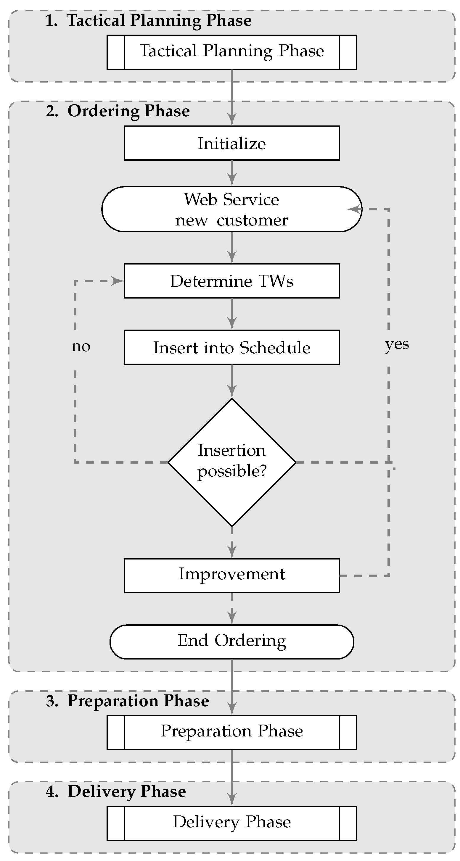An up-to-date taxonomic review of meta-heuristics for the most common variants of the vehicle routing problem can be found in Elshaer and Awad [34]. To efficiently deal with the ordering process, we propose to split the computations during the ordering phase into the following four steps (summarized in Figure 1).

3.1.1. Initialization Step

In the first step, the web service is being prepared to accept customer requests. Therefore, a new VRPTW instance is created, including all available vehicles with corresponding operation times. Since no orders have been placed yet, this results in an empty delivery schedule with a fixed fleet of vehicles.

3.1.2. Determination Step

When a new customer wants to place an order, the system has to determine the available delivery time windows that can be offered to this customer. This process has to be performed in milliseconds as customers are usually impatient when they have to wait for technical reasons. Note that for calculating the availabilities of time windows, the routing service has to calculate the travel times between all pairs of customers based on their provided addresses. The underlying mathematical problem of this step is the slot optimization problem (SOP) [23].

Optionally, for reasons of profit-maximizing, some available time windows can be hidden from the customer or be offered at different rates. In this work, we do not consider any (dynamic) slotting and pricing because the policy of our partnering grocery chain is to offer available time slots on a “first-come-first-served” basis, and each customer is accepted if possible. Nevertheless, we refer to Section 2.3, which provides a brief literature review about this topic.

3.1.3. Insertion Step

Given the list of time slots (determined in the previous step), the customer now chooses his or her preferred one. As it can take some time for the customer to decide on a time window or because many customers are booking simultaneously, the system must double-check if the selected time slot is still available. If the answer is yes, the customer can be added to the working schedule. If the answer is no, the system calls the determination step again to find an updated set of available time windows for the customer. This must be performed every time a customer wants to place an order. Note that we do not allow any simultaneous processing of the schedule to avoid queuing issues.

3.1.4. Improvement Step

In the last step, optimization techniques are applied to improve the schedule. These are important for two reasons: (a) to offer as many time windows as possible to the customers; (b) to serve as many customers as possible. This can be achieved by changing the assignments of customers to vehicles and, furthermore, by improving the routes of the delivery vehicles. We choose to minimize the total travel time as the objective function as this has proven to be reasonable in practice. During times with high customer frequencies, the improvement step can also be skipped or only invoked after a certain number of insertion steps to further improve the run time. At any time of the process, we allow for having exactly one working schedule in the system.

The time window determination step, as well as the insertion step, requires solving a feasibility version of the VRPTW. In contrast to that, the optimization version of the VRPTW must be solved during the improvement step.

Our approach is aimed at accepting as many customers as possible on a “first-come-first-served” basis, while offering each customer the largest possible selection of delivery time windows. Ideally, the working schedule would contain few large chunks of idle time rather than many short ones. As this is intractable to model in practice, we choose the total travel time as the objective function to avoid introducing an unnecessarily complicated model. Although Bent and Van Hentenryck [35] show that the use of a consensus function in their multiple-scenario approach results in more robust schedules and the acceptance of more customers, their approach is not applicable to our problem, as maintaining several scenarios would introduce additional complexity and require too much computational effort.

3.2. Vehicle Routing Problem with Time Windows

The vehicle routing problem with time windows (VRPTW) is concerned with finding a delivery schedule having the minimal total travel time for a fleet of vehicles with given capacity constraints to deliver goods to customers within assigned time windows. The problem is known to be NP-hard [36].

A VRPTW instance is defined by a set of customers $\mathcal{C},\left|\mathcal{C}\right|=p$, with a corresponding order weight function $c:\mathcal{C}\to {\mathbb{R}}^{>0}$, and a service time function $s:\mathcal{C}\to {\mathbb{R}}^{>0}$. In the considered AHD service, the individual items of an order $a\in \mathcal{C}$ are consolidated into several boxes of fixed size. The number of required boxes defines the corresponding order weight $c\left(a\right)$.

Secondly, the VRPTW consists of a set of time windows $\mathcal{W}=\left\{1,\dots ,q\right\}$, where each time window $u\in \mathcal{W}$ is defined through the times of its begin and end $(B_u,E_u)$. We assume that the time windows are unique, i.e., there do not exist time windows $u,v\in \mathcal{W},u\ne v$ with $B_u=B_v$ and $E_u=E_v$. We consider overlapping and non-overlapping time windows. Two time windows u and v are non-overlapping if and only if $E_u\le B_v$ or $E_v\le B_u$. Further, a function $w:\mathcal{C}\to \mathcal{W}$ is given that assigns to each customer a time window, during which the delivery vehicle has to arrive at the customer. All vehicles depart from and return to a depot d. The travel time between all points $a\in V=\mathcal{C}\cup \left\{d\right\}$ is given by a function $t:V\times V\to {\mathbb{R}}^{\ge 0}$, where we set the travel time from a customer a to itself to 0, i.e., $t(a,a)=0,a\in V$.

Each vehicle has an assigned tour. A tour $\mathcal{A}=(1,2,\dots ,n)$ contains n customers in the order they are visited by the vehicle and has an assigned capacity $C_{\mathcal{A}}$. Furthermore, each tour $\mathcal{A}$ has assigned start and end times that we denote as start${}_{\mathcal{A}}$ and end${}_{\mathcal{A}}$, respectively. Hence, the vehicle assigned to tour $\mathcal{A}$ can leave from the depot d no earlier than start${}_{\mathcal{A}}$ and must return to the depot no later than end${}_{\mathcal{A}}$. A schedule $\mathcal{S}=\left\{\mathcal{A},\mathcal{B},\dots \right\}$ consists of $\left|\mathcal{S}\right|=m$ tours.

3.3. Arrival Times and Feasibility

In this section, we define the feasibility of a schedule as well as the feasibility of inserting a new order into an existing schedule.

3.3.1. Earliest and Latest Arrival Times

We consider a fixed tour $\mathcal{A}=(0,1,\dots ,n,n+1)$, where 0 and $n+1$ denote the depot d and $(1,\dots ,n)$ denote the customers assigned to the tour. We use the concept of earliest and latest arrival time $e_i$ and ${\ell }_i$, as in reference [37], which give the earliest (latest) time at which the vehicle may arrive at customer i, while not violating time window and travel time constraints on the remaining tour:

$$\begin{array}{cccc}\hfill & e_0:=star{t}_{\mathcal{A}},\hfill & \hfill & e_{j+1}:=max\left\{B_{w(j+1)},e_j+s\left(j\right)+t(j,j+1)\right\},j\in {[n-1]}_0,\hfill \\ \hfill & \hfill & & e_{n+1}:=e_n+s\left(n\right)+t(n,n+1),\hfill \\ \hfill & {\ell }_{n+1}:=en{d}_{\mathcal{A}},\hfill & \hfill & {\ell }_{j-1}:=min\left\{E_{w(j-1)},{\ell }_j-t(j-1,j)-s(j-1)\right\},j\in \left[n\right]\setminus \left\{1\right\},\hfill \\ \hfill & \hfill & & {\ell }_0:={\ell }_1-t(0,1).\hfill \end{array}$$

Here, we assume $s\left(0\right)=s(n+1)=0$.

Following the definitions, vehicles always leave as early as possible from the depot. This generates unnecessary idle time before serving the first customer of a tour. Hence, once the delivery schedule is finalized, we alter the start times of the vehicles accordingly.

A schedule $\mathcal{S}$ is feasible if all its tours are feasible. A tour $\mathcal{A}$ is feasible if it satisfies both of the following conditions:

$$\begin{array}{ccc}\hfill & e_i\le E_{w\left(i\right)},i\in \left[n\right]\wedge e_{n+1}\le en{d}_{\mathcal{A}},\hfill & \hfill \mathrm{TFEAS}(\mathcal{A}),\\ \hfill & \sum _{i\in \left[n\right]}c\left(i\right)\le C_{\mathcal{A}},\hfill & \hfill \mathrm{CFEAS}(\mathcal{A}).\end{array}$$

While TFEAS($\mathcal{A}$) ensures that the arrival times at each customer assigned to tour $\mathcal{A}$ are within their assigned time windows, CFEAS($\mathcal{A}$) guarantees that the capacity of $\mathcal{A}$ is not exceeded. Note that we do not need to check for TFEAS($\mathcal{A}$) if $B_{w\left(i\right)}\le e_i,i\in \left[n\right],$ as this is ensured by the definition of $e_i$.

3.3.2. Insertion Points

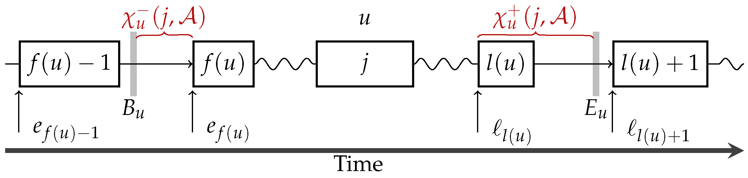
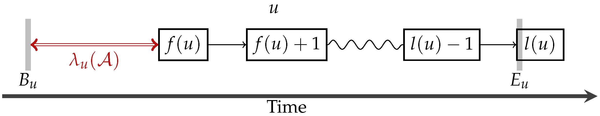
The set $\Theta (j,\mathcal{A})$ is required for the approaches applied in the time window determination step and defines after which customers we try to insert customer j into $\mathcal{A}$ during its (pre)assigned time slot. Accordingly, we define:

$$\begin{array}{cc}\hfill & \Theta (j,\mathcal{A}):=[{\Theta }^{-}(j,\mathcal{A}),{\Theta }^{+}(j,\mathcal{A})],\hfill \end{array}$$

where

$$\begin{array}{c}{\Theta }^{-}(j,\mathcal{A}):=\underset{i\in {\left[n\right]}_0}{min}\{i:B_{w\left(j\right)}+s\left(j\right)\le {\ell }_i\},\hfill \end{array}$$

(1)

$$\begin{array}{cc}\hfill & {\Theta }^{+}(j,\mathcal{A}):=\underset{i\in {\left[n\right]}_0}{max}\{i:e_i+s\left(i\right)\le E_{w\left(j\right)}\}.\hfill \end{array}$$

(2)

The index ${\Theta }^{-}(j,\mathcal{A})$ defines the first customer (or the depot) on tour $\mathcal{A}$ after which customer j could potentially be inserted. Likewise, ${\Theta }^{+}(j,\mathcal{A})$ defines the last customer. Clearly, if ${\Theta }^{-}(j,\mathcal{A})>{\Theta }^{+}(j,\mathcal{A})$, the insertion of j during $w\left(j\right)$ is infeasible.

3.3.3. Feasibility of an Insertion

The feasibility of the possible insertion points $\Theta (j,\mathcal{A})$ can be checked easily with earliest and latest arrival times, e.g., see reference [37]. Similar to the definitions above and with the help of $e_i$ and ${\ell }_i,i\in \mathcal{A}$, we define the earliest and latest arrival time ${\tilde{e}}_{j,i}$ and ${\tilde{\ell }}_{j,i}$ for inserting a new customer $j\notin \mathcal{A}$ after $i\in \Theta (j,\mathcal{A})\subseteq \mathcal{A}$ within the (pre)assigned time window $w\left(j\right)$ as follows:

$$\begin{array}{cc}\hfill & {\tilde{e}}_{j,i}:=max\left\{B_{w\left(j\right)},e_i+s\left(i\right)+t(i,j)\right\},\hfill \\ \hfill & {\tilde{\ell }}_{j,i}:=min\left\{E_{w\left(j\right)},{\ell }_{i+1}-t(j,i+1)-s\left(j\right)\right\}.\hfill \end{array}$$

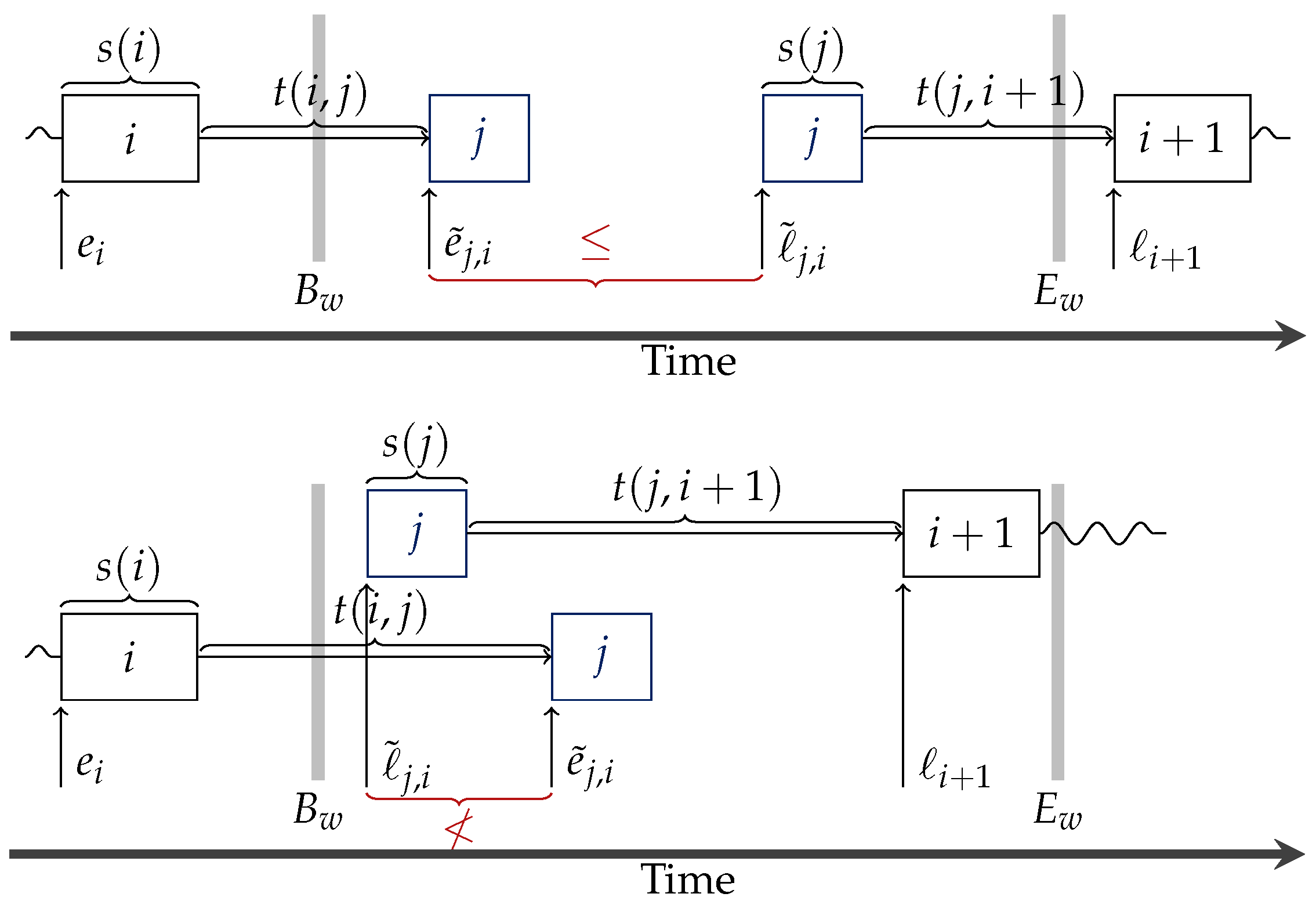
Thus, customer j can be inserted between customers i and $i+1$, such that j and all subsequent customers of $\mathcal{A}$ can be served within their assigned time windows if and only if the following condition holds.

$$\begin{array}{cccc}\hfill & {\tilde{e}}_{j,i}\le {\tilde{\ell }}_{j,i},\hfill & \hfill & \mathrm{TFEAS}(j,i,\mathcal{A}),\hfill \end{array}$$

We refer to Figure 2 for an illustration.

Additionally, we must check if the sum of the weights of the customer orders assigned to tour $\mathcal{A}$ does not exceed its capacity $C_{\mathcal{A}}$. The insertion of j into tour $\mathcal{A}$ is feasible with respect to capacity if the following condition holds:

$$\begin{array}{cccc}\hfill & \sum _{i\in \left[n\right]}c\left(i\right)+c\left(j\right)\le C_{\mathcal{A}},\hfill & \hfill & \mathrm{CFEAS}(j,\mathcal{A}).\hfill \end{array}$$

Assuming that all earliest (latest) arrival times and the sum of order weights on a tour $\mathcal{A}$ have already been calculated, TFEAS($j,i,\mathcal{A}$) and CFEAS($j,\mathcal{A}$) allow to check the feasibility of a possible insertion into a given time window in $\mathcal{O}\left(1\right)$ time provided that the sequence of $\mathcal{A}$ (except for j) stays the same. If the feasibility check was successful and we decide to insert j, we obtain a new tour $\tilde{\mathcal{A}}=\mathcal{A}{+}_{i}j=(0,1,\dots ,i,j,i+1,\dots ,n,n+1)$. Customer j is then assigned to index $i+1$, and all indices of succeeding customers are incremented. Clearly, the earliest and latest arrival times and the sum of order weights of the modified tour must be updated. This requires $\mathcal{O}\left(n\right)$ time [38]. In general, there exist cases where a feasible insertion of j is only possible when the order of $\mathcal{A}$ is changed, which makes the problem NP-hard.

3.4. Slot Optimization Problem

With the introduced notation, we can recall the formal definition of the slot optimization problem (SOP) [23], which arises in the time window determination step. We are given a feasible schedule $\mathcal{S}$ containing all scheduled customers $\mathcal{C}$, a new customer $j,j\notin \mathcal{C}$, and the given set of time slots $\mathcal{W}$. Then, the SOP asks for the largest set of time slots ${\mathcal{T}}_j\subseteq \mathcal{W}$ such that j can be serviced during each delivery slot $u\in {\mathcal{T}}_j$ by at least one vehicle of the fleet, while assuring that all other scheduled orders stay within their assigned time slot. Hence, the objective is to maximize $\left|{\mathcal{T}}_j\right|$.

In more detail, the SOP aims to find at least one feasible schedule for each of the VRPTW instances consisting of the already scheduled customers $\mathcal{C}$ and the new customer j being temporarily assigned to one of the time windows $u\in \mathcal{W}$. Choosing one delivery slot for the new customer order makes the SOP equivalent to the feasibility version of the VRPTW. As the VRPTW is strongly NP-hard [39], the SOP is also strongly NP-hard and consists of several feasibility problems that are all strongly NP-complete.

4. Algorithms for the VRPTW

We start with introducing the algorithms that we use to tackle our proposed AHD system in Section 4.1, Section 4.2, Section 4.3, Section 4.4. Then, in Section 4.5 we describe how they are combined and applied to the different steps of the ordering phase.

4.1. Simple Insertion Heuristic

The simple insertion heuristic, based on Savelsbergh [22], takes a new customer j and a tour $\mathcal{A}$, and tries to insert j into the temporarily assigned time window $w\left(j\right)\in \mathcal{W}$. It stops as soon as it finds a feasible insertion point $i\in \Theta (j,\mathcal{A})$, i.e., when TFEAS($j,i,\mathcal{A}$) and CFEAS($j,\mathcal{A}$) hold. Note, since the order of customers is not altered, the procedure has a linear run time $\mathcal{O}\left(\right|\mathcal{A}\left|\right)$. We iteratively apply the simple insertion heuristic to all time windows $u\in \mathcal{W}$ and all tours $\mathcal{A}\in {\mathcal{S}}_u$ to calculate the set of time windows that can be offered to the new customer j. ${\mathcal{S}}_u$ defines the set of tours including the time window u, i.e., $\mathcal{A}\in {\mathcal{S}}_u$ if and only if $star{t}_{\mathcal{A}}\le B_u<E_u\le en{d}_{\mathcal{A}}$. A time window is considered as being available if at least one feasible insertion point can be found.

4.2. Local Search Heuristic

We apply a local search heuristic that uses the following neighborhoods for exchanging customer orders between two tours. The 1move  neighborhood moves a customer j from a tour $\mathcal{A}$ to another tour $\mathcal{B}$, $\mathcal{A}\ne \mathcal{B}$. If at least one feasible insertion position for j in $\mathcal{B}$ is found, i.e., TFEAS($j,i,\mathcal{B}$) and CFEAS($j,\mathcal{B}$) hold, which additionally decreases the total travel time of the delivery schedule, we denote the 1move   as improving. The 1swap  neighborhood exchanges two customers between two different tours, e.g., it exchanges $j\in \mathcal{A}$ with $i\in \mathcal{B}$. Again, if a feasible swap with a decreased total travel time is found, we denote the 1swap   as improving. Savelsbergh [22] uses similar neighborhoods, calling them Relocate and Exchange. Clearly, if no improving 1move  (1swap) can be found for a pair of tours $(\mathcal{A},\mathcal{B})\in \mathcal{S}$, $\mathcal{A}\ne \mathcal{B}$, and both tours have not been modified meanwhile, then there is no need to perform those operations for this pair of tours again. Preliminary experiments showed that the computation times are reduced by a third by storing this information during the updates.

4.3. Adaptive Neighborhood Search Heuristic

We extend the ANS for solving the SOP proposed by Hungerläender et al. [23] such that it can also be applied to overlapping time windows. This results in different interdependencies between time windows as well as slightly weaker (in)feasibility conditions. In the following, we state all definitions required to describe our ANS.

4.3.1. First/Last Customer

For a given tour $\mathcal{A}$ we define the first and last customer belonging to a given time slot $u\in \mathcal{W}$ as

$$\begin{array}{cc}\hfill & f\left(u\right):=\underset{i\in \left[n\right]}{min}\left\{i:B_u\le B_{w\left(i\right)}\le E_{w\left(i\right)}\le E_u\right\},\hfill \\ \hfill & l\left(u\right):=\underset{i\in \left[n\right]}{max}\left\{i:B_u\le B_{w\left(i\right)}\le E_{w\left(i\right)}\le E_u\right\}.\hfill \end{array}$$

If above sets are empty, then the indices are not defined, i.e., $\left[f\right(u),l(u\left)\right]=\varnothing$. In case of non-overlapping time slots and if $w\left(j\right)=u,j\notin \mathcal{A},$ and u is not empty, i.e., there is at least one customer $i\in \mathcal{A}$ assigned to u, the following statement holds:

$$\Theta (j,\mathcal{A})\subseteq \left\{f\right(u)-1,\dots ,l(u\left)\right\}.$$

4.3.2. Neighborhoods

Our ANS heuristic considers two different neighborhoods for a time window $u\in \mathcal{W}$ and a tour $\mathcal{A}\in \mathcal{S}$.

• inside includes all operations with customers inside u:
  $in(u,\mathcal{A}):=\{i\in \mathcal{A}:i\in [f\left(u\right),l\left(u\right)\left]\right\};$
• outside represents operations with customers outside u:
  $out(u,\mathcal{A}):=\mathcal{A}\setminus \left(in\right(u,\mathcal{A})\cup \{0,n+1\left\}\right).$

The inside of u consists of customers $i\in \mathcal{A}$ that are: (a) assigned to time window $u=w\left(i\right)$; (b) assigned to a time window that is included in u: $s_u\le s_{w\left(i\right)}\le e_{w\left(i\right)}\le e_u$; or (c) captured by customers of u (or its included time windows), e.g., there exist two customers $j,k\in \mathcal{A}$ with $w\left(j\right)=w\left(k\right)=u$ such that $j<i<k$ and $i,j,k\in \left[n\right]$.

Clearly, $in(u,\mathcal{A})$ is dependent on the actual tour sequence. However, in case of non-overlapping time windows, the customers inside u are exactly those who are assigned to u, i.e., $in(u,\mathcal{A})=\{i\in \mathcal{A}:w(i)=u\}$.

In Figure 3, we illustrate the definitions that have been introduced so far. We display the position of the first $f\left(u\right)$ and last customers $l\left(u\right)$ of u in case of overlapping time windows. Moreover, we indicate the positions of the insertion points ${\Theta }^{-}(j,\mathcal{A})$ and ${\Theta }^{+}(j,\mathcal{A})$ (vertical lines). In the given example, we notice that $\Theta (j,\mathcal{A})$ and $\left\{f\right(u)-1,\dots ,l(u\left)\right\}$ differ as also the insertion of j after customer $l\left(u\right)+1$ must be considered. Furthermore, we observe that customer $f\left(u\right)+2$ is inside u although being assigned to time window $u-1$.

4.3.3. Loss and Free Time

For a tour $\mathcal{A}$ and a new customer j who has to be inserted into time slot u, we define

$$\begin{array}{cc}\hfill {\chi }_u^{-}(j,\mathcal{A})& :=max\left(e_{f\left(u\right)},\underset{i\in \Theta (j,\mathcal{A}),i\le f\left(u\right)}{max}{\tilde{e}}_{j,i}\right)-B_u,\hfill \\ \hfill {\chi }_u^{+}(j,\mathcal{A})& :=E_u-min\left({\ell }_{l\left(u\right)},\underset{i\in \Theta (j,\mathcal{A}),i\ge l\left(u\right)}{min}{\tilde{\ell }}_{j,i}\right).\hfill \end{array}$$

The value ${\chi }_u^{-}$ corresponds to the amount of time that is “lost” at the beginning of time slot u. This can be caused by the service time required for the last customer order before (outside) u or the travel time needed for going from that customer to the first customer inside u. Similarly, ${\chi }_u^{+}$ corresponds to the loss of time at the end of time slot u caused by the time required for traveling to the first customer after (outside) u or the service time at the last customer inside u.

Further, we denote ${\chi }_u(j,\mathcal{A}):={\chi }_u^{-}(\mathcal{A},j)+{\chi }_u^{+}(j,\mathcal{A})$ as the loss time of time window u. In case that $\left[f\right(u),l(u\left)\right]=\varnothing$, the loss time is given by

$${\chi }_u(j,\mathcal{A})=\underset{i\in \Theta (j,\mathcal{A})}{max}\left(({\tilde{e}}_{j,i}-s_u)+(e_u-{\tilde{\ell }}_{j,i})\right).$$

Figure 4 illustrates the values ${\chi }_u^{-}(j,\mathcal{A})$ and ${\chi }_u^{+}(j,\mathcal{A})$ for a tour with non-overlapping time windows. Clearly, if ${\chi }_u(j,\mathcal{A})=0$, then a violation of TFEAS($\mathcal{A}$) for j can only be repaired by removing (exchanging) customers that are inside u.

Furthermore, we want to quantify the amount of service and travel time that is needed for inserting j during time window u. For a given tour $\mathcal{A}$, the free time of time slot u is defined as

$$\begin{array}{c}\hfill {\lambda }_u\left(\mathcal{A}\right):=\underset{\left(I\right)}{\underbrace{\left(E_u-B_u\right)}}-\underset{\left(II\right)}{\underbrace{\sum _{i=f\left(u\right)}^{l\left(u\right)-1}\left(s\left(i\right)+t(i,i+1)\right)}},\end{array}$$

where $\left(I\right)$ is the length of u and $\left(II\right)$ is the amount of service and travel time that must be handled within u. In case that the indices $f\left(u\right)$ and $l\left(u\right)$ are not defined, i.e., $in(u,\mathcal{A})=\varnothing$, term $\left(II\right)$ is set to 0. In Figure 5, we provide an illustration of the free time.

Considering non-overlapping time windows, the insertion of customer j after a customer $i\in \{f\left(u\right)-1,\dots ,l(u\left)\right\}$ requires an additional amount of (travel and service) time that must be handled within time window u and can be calculated by ${\lambda }_u\left(\mathcal{A}\right)-{\lambda }_u\left(\mathcal{A}{+}_{i}j\right)$. This assumes that all customers between $f\left(u\right)$ and $l\left(u\right)$ can be moved arbitrarily (while maintaining their sequence) within time slot u, i.e., all customers assigned to u can be seen as one consecutive block, the length of which is given by $\left(II\right)$. Hence, the above statement is weakened in the case of overlapping time windows, as some customers inside u may be restricted by their assigned time windows such that no consecutive block of customers can be formed. Therefore, a larger amount of time than $\left(II\right)$ may be required for tour $\mathcal{A}$ after the insertion of customer j.

4.3.4. Feasibility and Infeasibility Conditions

The insertion of j into $\mathcal{A}$ is infeasible if the following holds:

$$\begin{array}{c}\hfill \underset{i\in \Theta (j,\mathcal{A})}{max}{\lambda }_u\left(\mathcal{A}{+}_{i}j\right)<0.\end{array}$$

(3)

We note that condition (1) solely depends on the customers inside u. Hence, in case of non-overlapping time windows, it is only dependent on the customers assigned to time slot u. Moreover, in case of non-overlapping time slots, the insertion of j into $\mathcal{A}$ is feasible for at least one insertion position if the following inequality holds:

$$\begin{array}{c}\hfill \underset{i\in \Theta (j,\mathcal{A})}{max}{\lambda }_u\left(\mathcal{A}{+}_{i}j\right)-{\chi }_u(\mathcal{A},j)\ge 0.\end{array}$$

(4)

Note that the statement does not hold in the case of overlapping time windows.

4.3.5. Algorithm

Finally, we can concisely describe the details of our ANS for the SOP as follows. We temporarily assign the new customer j to each time window $u\in \mathcal{W}.$ For each tour $\mathcal{A}\in {\mathcal{S}}_u$ we apply the steps described below, which try to insert j into $\mathcal{A}$ within its assigned time window $w\left(j\right)=u$. If this is possible, u is added to the set of available time windows ${\mathcal{T}}_j\subseteq \mathcal{W}$.

In step 1, we ensure that the current tour $\mathcal{A}$ fulfills CFEAS($j,\mathcal{A}$). If ${\displaystyle \sum _{i\in \left[n\right]}}c\left(i\right)+c\left(j\right)>C_{\mathcal{A}}$ holds, then customer a cannot be feasibly inserted into tour $\mathcal{A}$. In this case, we have to reduce the overall weight ${\displaystyle \sum _{i\in \left[n\right]}}c\left(i\right)$ of $\mathcal{A}$. This is achieved by applying local search operations 1move  and 1swap, while as few operations as possible are used. Therefore, as much weight as possible is moved in each step and the operations stop once there is sufficient spare capacity on $\mathcal{A}$ to insert j, i.e., ${\displaystyle \sum _{i\in \left[n\right]}}c\left(i\right)+c\left(j\right)\le C_{\mathcal{A}}$ holds. If we do not succeed in modifying $\mathcal{A}$ such that CFEAS($j,\mathcal{A}$) holds, we terminate.

In step 2, we aim to increase the free time ${\lambda }_u\left(\mathcal{A}\right)$ through local search operations within inside until the infeasibility condition (1) does not hold anymore. ${\lambda }_u\left(\mathcal{A}\right)$ is increased by applying as few operations as possible. That way, the previously optimized schedule ${\mathcal{S}}_u$ is not altered more than necessary. If a local optimum is reached, meaning no further improvements can be achieved by local search operations, and (1) is still satisfied, the algorithm stops because the following steps cannot result in a feasible insertion of the new customer.

Next, step 3 is concerned with reducing the loss time ${\chi }_u(j,\mathcal{A})$ of time slot u through local improvement operations within outside. The operations are applied until either the new customer order can be inserted into the tour, the loss time is equal to zero ${\chi }_u(j,\mathcal{A})=0$, or a local optimum is reached.

Finally, in step 4 we try to further increase the free time through local search operations within inside. The free time is increased until either the insertion of customer j is possible or a local optimum (of the free time objective) is reached and hence, we are not able to insert j within time slot u.

Note that we apply local search operations during steps 2–4 only if CFEAS($j,\mathcal{A}$) still holds. Further, we apply local search operations during step 3 only if the infeasibility condition (1) does not hold for the resulting tour $\mathcal{A}$.

4.4. Exact Approach for Solving a Sub-Problem

In this subsection we consider the TSPTW, a sub-problem of the VRPTW, which was first introduced by Savelsbergh [22]. The TSPTW is concerned with minimizing the travel time of a single tour $\mathcal{A}\in \mathcal{S}$ of the VRPTW, while all other tours in the schedule are fixed. Hungerländer and Truden [40] give two competitive MILP formulations for the TSPTW that we utilize in our hybrid approaches (described in Section 4.5): (i) a general model that can be applied to any TSPTW instance (having asymmetric travel times) regardless of the structure of the defined time windows $\mathcal{W}$; (ii) a second model that is tailored to the TSP with structured time windows (TSPsTW). It is assumed that the time windows $\mathcal{W}$ are pair-wise, non-overlapping, and that the number of customers $\left|\mathcal{C}\right|=p$ is much larger than the number of time windows $\left|\mathcal{W}\right|=q$, i.e., $p\gg q$, and therefore typically several customers are assigned to the same time window. This assumption allows a simplified MILP formulation that performs significantly better.

We refer the reader to the following paper in reference [40] for details on both MILPs as well as a short computational study that compares both formulations. In contrast to the VRPTW, the TSP(s)TW is concerned with single tours. Hence, it is unnecessary to include a capacity constraint in the MILP models, as the sum of order weights of a tour is independent of the actual sequence of the customers on the tour.

4.5. Solution Approaches

In this subsection, we describe how we combine the heuristics and MILPs presented above such that we can conduct the different steps of the ordering phase sufficiently fast.

First, in the determination step, we aim to quickly identify all time windows ${\mathcal{T}}_j\subseteq \mathcal{W}$ during which a new customer j can be inserted into (at least one of) the current tours. We compare to the following approaches.

• Simple insertion heuristic;
• ANS heuristic;
• A feasibility version of the suggested MILPs for solving the TSP(s)TW, which are applied for each time slot $u\in \mathcal{W}$ and for each $\mathcal{A}\in {\mathcal{T}}_u$.

Once customer j has selected a time window $u\in {\mathcal{T}}_j$, in the insertion step we double-check its availability in the same way as in the determination step and then immediately insert j into u at the best insertion point found. In contrast to the determination step, we run the simple insertion heuristic or the ANS over all tours and all insertion points and select the feasible insertion point that results in the lowest increase of the total travel time of the schedule. Thus, we do not stop the algorithm once the first feasible insertion point is found. In the case of the TSP(s)TW MILPs we apply their standard formulations for finding an optimal tour after the insertion of j, rather than their corresponding feasibility versions.

In the improvement step, we aim to reduce the total travel time of the schedule. We compare the following approaches.

• 1move  + (1swap). The computationally cheap yet quite effective local search heuristic builds the foundation of the improvement step. We apply 1move   (and 1swap)   operations, where we focus on the 1move   operations if possible, because they are computationally cheaper and, in general, more effective than 1swap   operations. We stop our local search heuristic once we reach a local minimum of the objective function with respect to the selected neighborhood;
• 1move  + 1swap  + TSP(s)TW. After applying the local search heuristic, we additionally run our TSP(s)TW MILP on all tours that have changed since the last improvement step. We use the current tours of our delivery schedule as the initial solution for TSP(s)TW MILP. While 1move and 1swap exchange customers between different tours, the TSP(s)TW MILP re-orders them within the tours, which makes it a useful complement to the local search heuristics. In practice, optimizing the single tours of a schedule to optimality has proven to be critical to ensure driver satisfaction as it guarantees that drivers do not encounter any inefficiencies on their routes.

Above presented improvement procedures are arranged in ascending order with respect to their computational effort.

During the ordering phase, the proposed local search procedures only perform improving operations. However, the algorithms can be simply altered to a simulated annealing approach [41] by allowing also non-improving operations. However, this is more suitable for the preparation phase, when more time is available for improving the delivery schedule.

5. Computational Study and Analysis

We want to provide a performance evaluation of the different steps and approaches of the ordering phase. First, in Section 5.1, we describe the design of our test instances. In Section 5.2, we analyze how well, in terms of run time and solution quality, the different approaches for the time window determination step perform. Then, we compare the different improvement approaches in Section 5.3. Finally, in Section 5.4, we compare the performances of different combinations of approaches for the determination and the improvement step.

5.1. Design of the Instances

The benchmark instances are derived from those originally proposed by reference [13]. They are designed to reproduce the characteristics of an online grocery shopping service offered by an international grocery retailer.

Each instance corresponds to one delivery region that is served by one depot, which has its assigned fleet of vehicles. All instances are based on a 20 $\mathrm{k}$$\mathrm{m}$× 20 $\mathrm{k}$$\mathrm{m}$ square grid. A total of 80% of the customer locations have been randomly assigned to 15 clusters. The center (location) of each cluster $\mu =({\mu }_x,{\mu }_y)$ is sampled from a two-dimensional uniform distribution. The shape of each cluster is defined by the covariance matrix $\Sigma =\left(\begin{array}{cc}{{\sigma }_x}^2& 0\\ 0& {{\sigma }_y}^2\end{array}\right)$, where ${{\sigma }_x}^2$ and ${{\sigma }_y}^2$ both follow a uniform distribution. Furthermore, the clusters have been rotated by a random angle between 0 and $2\pi$. Customer locations have been sampled from the multivariate normal distribution $N(\mu ,\Sigma )$ of the assigned cluster and all coordinates have been rounded to integers. The remaining 20% of the locations are sampled from a two-dimensional uniform distribution. The numbering of the customers is randomly permuted.

We consider two different placements of the depot: (a) at the center of the grid; (b) at the center of the top-left quadrant. In each test set-up, there are equally many instances for both variants. Each vehicle has a loading capacity of 200 units. The order weights of customers have been sampled from a truncated normal distribution with a mean of 7 and standard deviation of 2, where the lower bound is 1 and the upper bound is 15. The service time of each customer is 5. All tours have the same start and end times while vehicle operation times are set such that they do not overly restrict the problem.

We apply a very simple customer choice model to simulate the customer’s choice if they place an order or not after being presented the selection of time windows. Similar to Cleophas and Ehmke [28], every customer has just one desired delivery time window (defined in the benchmark instance). The customer refuses to place an order if this preferred time window is not offered. Furthermore, we assume that all delivery time windows are equally prominent among customers (randomly selected from $\mathcal{W}$) to obtain unbiased results that allow for an easier identification and clearer interpretation of the key findings.

We define three sets of delivery time windows $\mathcal{W}$: (a) ${\mathcal{W}}_{\mathrm{NO}}$: 10 non-overlapping time windows with a length of 1 h each, e.g., 08:00–09:00, 09:00–10:00, etc. (b) ${\mathcal{W}}_{\mathrm{OV}1.5}$: 10 overlapping time windows with a length of 1.5 h each (except for the last time window, which has a 1 h length), where each window overlaps the preceding time window by 30, e.g., 08:00–09:30, 09:00–10:30, etc. (c) ${\mathcal{W}}_{\mathrm{OV}3}$: 12 overlapping time windows, consisting of nine windows with a length of 1 h each, 08:00–09:00, 10:00–11:00, …, 16:00–17:00 and (as used by Köhler et al. [21]) three time windows of 3 h length, morning: 08:00–11:00, noon: 11:00–14:00, afternoon: 14:00–17:00.

In summary, our assumptions were chosen to find a good compromise between realistic instances and enabling a concise description and interpretation of the experimental set-up. All experiments were performed on an Ubuntu 14.04 machine powered by an Intel Xeon E5-2630V3 @ 2.4 GHz 8 core processor and 132 GB RAM. We implemented all algorithms in Java Version 8 and used Gurobi 8.1.0 as the MILP solver in single-thread mode. Parallelization of the applied methods is not considered. We run each experimental configuration on 100 instances and report average values. Note that the absence of overlapping time windows allows for the use of a more efficient MILP formulation of the TSPTW for ${\mathcal{W}}_{\mathrm{NO}}$ than for ${\mathcal{W}}_{\mathrm{OV}1.5}$ and ${\mathcal{W}}_{\mathrm{OV}3}$ (see Section 4.4).

5.2. Comparing Approaches for the Determination Step

In this subsection, we evaluate the performance of different approaches for the time window determination step, i.e., we compare the simple insertion heuristic, the ANS heuristic, and the TSP(s)TW insertion approach in terms of run time and solution quality.

To allow a proper comparison of the methods for solving the SOP, we constructed instances which consist of (a) a feasible schedule that contains p customers, and (b) a new customer order for which the availability of delivery time slots must be decided. To create SOP instances for benchmarking, we had to create feasible delivery schedules that are already filled with orders. Hence, we created delivery schedules by iteratively trying to insert 2000 customers into each schedule. The simple insertion heuristic was used to conduct the feasibility checks. The number of customers that are contained in the resulting schedule is denoted by $\widehat{p}$. We consider $\widehat{p}$ as being a sufficiently good approximation of the maximal number that can be inserted into a schedule considering a given configuration. Hence, we distinguish two scenarios: (i) in the first scenario, we perform no optimization between the insertion steps, and (ii) in the second scenario, the schedule is re-optimized by applying 1move after each customer insertion. This reduces the total travel time of the schedule. We restrict the improvement step to the most simple approach to avoid unwanted bias when evaluating the performance of the different approaches for the determination step. In general, the schedules in the second scenario contain more orders while utilizing the same number of vehicles.

Since the practical hardness of the SOP increases as the schedules are filled up with customers, we consider SOP instances with different fill levels. The fill level f of a schedule is defined as the ratio between the number of customers p in the schedule and the maximal number of customers $\widehat{p}$ that can be inserted into the schedule. For benchmarking at a given fill level f, we select the schedule that was generated by above described process, which contained $p=\lceil f·\widehat{p}\rceil$ orders. For each generated instance, we solve the SOP using the simple insertion heuristic, the TSP(s)TW insertion n approach, and the proposed ANS heuristic. In order to investigate the differences between the considered methods, we analyze their performance on all three sets of time windows (${\mathcal{W}}_{\mathrm{NO}}$, ${\mathcal{W}}_{\mathrm{OV}1.5}$, ${\mathcal{W}}_{\mathrm{OV}3}$), instance sizes, and fill levels. Hence, we run tests on benchmark instances with 60 tours (vehicles) and consider fill levels of 85%, 90%, 95%, and 99%.

We report the number of feasible time slots found by each method and required run times (mm:ss.zzz) for all scenarios, i.e., optimized and non-optimized schedules. We report the results for ${\mathcal{W}}_{\mathrm{NO}}$ in

Table 1. Summary of the computational experiments concerning the approaches for the determination step using ${\mathcal{W}}_{\mathrm{NO}}$ considering non-optimized and 1move-optimized schedules.

${\mathcal{W}}_{\mathbf{NO}}$ (10 Windows)—60 Vehicles
	Non-Optimized Schedules				Optimized Schedules
Avg. $\widehat{p}$	408.0				1907.3
Fill level	85%	90%	95%	99%	85%	90%	95%	99%
Avg. run time
(mm:ss.zzz)
simple insertion	00:00.001	00:00.001	00:00.001	00:00.001	00:00.001	00:00.001	00:00.001	00:00.001
TSP(s)TW insertion	00:00.223	00:00.422	00:01.112	00:01.970	00:00.592	00:00.580	00:00.743	00:00.455
ANS	00:00.024	00:00.089	00:00.468	00:04.031	00:00.049	00:00.052	00:00.077	00:01.377
Avg. number
of feasible slots
Simple insertion	9.82	9.47	7.67	2.00	9.98	9.98	9.83	4.20
TSP(s)TW insertion	9.85	9.62	8.60	4.30	9.98	9.98	9.83	4.29
ANS	9.96	9.94	9.93	9.39	9.98	9.98	9.98	9.63
Combined	9.96	9.94	9.93	9.43	9.98	9.98	9.98	9.63

, for ${\mathcal{W}}_{\mathrm{OV}1.5}$ in

Table 2. Summary of the computational experiments concerning the approaches for the determination step using ${\mathcal{W}}_{\mathrm{OV}1.5}$ considering non-optimized and 1move-optimized schedules.

${\mathcal{W}}_{\mathbf{OV}1.5}$ (10 Windows)–60 Vehicles
	Non-Optimized Schedules				Optimized Schedules
Avg. $\widehat{p}$	628.0				1880.0
Fill level	85%	90%	95%	99%	85%	90%	95%	99%
Avg. run time
(mm:ss.zzz)
Simple insertion	00:00.001	00:00.001	00:00.001	00:00.001	00:00.001	00:00.001	00:00.001	00:00.001
TSP(s)TW	00:03.505	00:11.182	00:52.761	02:22.804	00:41.024	01:01.611	01:03.537	00:11.598
ANS	00:00.032	00:00.138	00:00.683	00:07.837	00:00.036	00:00.040	00:00.066	00:08.343
Avg. number
of feasible slots
Simple insertion	9.57	9.05	7.40	0.76	9.98	9.98	9.68	0.72
TSP(s)TW insertion	9.84	9.68	8.96	5.04	10.00	10.00	9.84	0.70
ANS	9.99	9.95	9.83	8.43	10.00	10.00	9.84	6.36
Combined	9.99	9.95	9.87	8.76	10.00	10.00	10.00	6.36

, and for ${\mathcal{W}}_{\mathrm{OV}3}$ in

Table 3. Summary of the computational experiments concerning the approaches for the determination step using ${\mathcal{W}}_{\mathrm{OV}3}$ considering non-optimized and 1move-optimized schedules.

${\mathcal{W}}_{\mathbf{OV}3}$ (12 Windows)–60 Vehicles
	Non-Optimized Schedules				Optimized Schedules
Avg. $\widehat{p}$	406.0				1897.9
Fill level	85%	90%	95%	99%	85%	90%	95%	99%
Avg. run time
(mm:ss.zzz)
Simple insertion	00:00.001	00:00.001	00:00.001	00:00.001	00:00.001	00:00.001	00:00.001	00:00.001
TSP(s)TW insertion	00:02.645	00:15.541	01:27.422	05:20.061	00:56.969	00:54.405	01:04.239	00:17.879
ANS	00:00.012	00:00.112	00:00.847	00:08.412	00:00.052	00:00.057	00:00.073	00:08.981
Avg. number
of feasible slots
Simple insertion	11.84	11.02	8.54	1.21	12.00	12.00	11.90	0.73
TSP(s)TW insertion	11.93	11.73	10.78	6.65	12.00	12.00	11.92	0.69
ANS	12.00	11.98	11.94	10.16	12.00	12.00	12.00	7.59
Combined	12.00	11.99	11.97	10.73	12.00	12.00	12.00	7.59

. Moreover, we report the number of feasible time slots that are found by combining the findings of all three methods, denoted as “combined” in the tables. Additionally, we report $\widehat{p}$, the number of customers at a 100% fill level. All reported numbers are average values over 100 instances each.

As a reference to compare against, we select the simple insertion heuristic. Both other methods, TSP(s)TW insertion and ANS, are entitled to find at least the delivery time slots that are determined by the simple insertion heuristic. This property is guaranteed due to the construction of those methods. Unfortunately, we can not provide an upper bound for the number of feasible delivery time slots as, to the best of our knowledge, there is no more powerful search method applicable for the SOP in the current literature. In our experiments, we restrict the ANS to 1move operations, as preliminary experiments showed that allowing 1swap operations yields unacceptably long run times (up to some minutes). Additionally, the results are only insignificantly better. Primarily, we notice that the simple insertion heuristic returns solutions for the SOP in less than one millisecond for all considered instances. At fill level (85%) the instances are still rather easy and, hence, the simple insertion heuristic determines nearly all time slots as being feasible. While the simple insertion heuristic still performs well at 90% and 95% on optimized schedules, it performs poorly on non-optimized schedules with the same fill levels due to the lower quality of the schedules.

Furthermore, we observe that the TSP(s)TW insertion approach yields a slight improvement over the simple insertion heuristic in terms of available time windows at 85–95%. However, a significant improvement can be observed when it is applied to non-optimized schedules at a 99% fill level. TSP(s)TW insertion shows acceptable run times for ${\mathcal{W}}_{\mathrm{NO}}$. In contrast, run times for ${\mathcal{W}}_{\mathrm{OV}1.5}$ and ${\mathcal{W}}_{\mathrm{OV}3}$ are between 3 s and nearly 4 and are thus unacceptable. Hence, considering these findings, the TSP(s)TW insertion turns out to be impractical for AHD systems. Moreover, we notice that the ANS yields significantly more feasible time slots than the simple insertion heuristic (and TSP(s)TW insertion) on non-optimized schedules at 95% and 99%. Similar behavior can be observed on optimized schedules at 99%. The run times of the ANS stay below 1 s for nearly all experiments with up to a 95% fill level. The ANS clearly performs best in terms of solution quality on instances having a 99% fill level, resulting in up to 11 times more available delivery time windows than with simple insertion. However, on those instances its run time reaches up to 9 s. It is worth pointing out that the performance of the ANS is nearly constant over all three sets of time windows, showing that it can also deal with instances having overlapping delivery time windows.

In general, we notice a slight performance drop of the ANS (compared to the TSP(s)TW insertion approach) when being applied non-optimized schedules compared to optimized schedules. This can be explained by the fact that identifying feasible time windows is less hard for non-optimized schedules as they contain less orders on average. Additionally, there is more potential for improvement when applying TSP(s)TW insertion as the single tours have not been improved in any way after inserting the customers. Additionally, we observe that “combined” shows only a marginal improvement over the ANS for optimized schedules. On the other hand, we notice a strong improvement of “combined” compared to the TSP(s)TW insertion approach and ANS for non-optimized schedules at a 99% fill level. This can be explained by the fact that the TSP(s)TW insertion approach has a larger potential of finding a feasible insertions (compared to the simple insertion heuristic) if the tours are of low quality (as there is more room to rearrange the tours) due to the already observed weaker performance of the ANS in this case.

Our experiments show that the ANS heuristic is capable of finding a larger number of feasible delivery slots than the simple insertion heuristic, requiring run times that are still well suited for AHD services when dealing with moderately sized problem instances. However, to efficiently tackle very large instances, the parallelization of the ANS is advised. In summary, the ANS heuristic is clearly the best method for solving the SOP when being concerned with the solution quality while the simple insertion heuristic is the method of choice in cases of tight run time restrictions.

5.3. Comparing Approaches for the Improvement Step

To compare the proposed improvement approaches, we perform experiments where we iteratively insert new customers into the schedule, simulating customers placing orders online. Due to the iterative benchmark set-up, we can insert the new order without double-checking the availability of the selected delivery time slot. Again, to avoid bias, we stick to the most simple approach for the determination step, the simple insertion heuristic. Then, for the improvement step we compute the following metrics:

• Average improvement over insertion step: the average reduction of the objective function when applying the optimization approaches to the schedule after inserting the new customer (given in percentage);
• Average improvement of the cost of insertion: the average reduction of the objective function relative to the increase of the objective function caused by inserting the new customer (given in percentage);
• Average number of TSPsTW MILPs solved;
• Average run time of each improvement strategy.

Additionally, we report the average total number of customer orders that have been inserted into the final schedules. Note that for the MILPs we set a time limit of 60 s.

5.3.1. Average-Sized Grocery Home Delivery Problems

First, we want to analyze the improvement approaches for instance sizes which we found to appear most commonly in practice. Hence, we consider 500 customers that are served by $16/18/20$ vehicles with a capacity of 200 units each. The number of used vehicles corresponds to the practical difficulty of the instances. The numbers are chosen such that the instances are reasonably difficult. In that sense, using 20 vehicles results in accepting nearly all 500 customers on average. These instances are designed to reflect the majority of delivery regions as they were encountered during our project with a leading supermarket chain. The results for these experiments are reported in

Table 4. Summary of the computational experiments for the improvement approaches considering instances with 500 customers.

Average-Sized Grocery Home Delivery Problems
	${\mathcal{W}}_{\mathrm{NO}}$			${\mathcal{W}}_{\mathrm{OV}1.5}$			${\mathcal{W}}_{\mathrm{OV}3}$
Vehicles	16	18	20	16	18	20	16	18	20
Avg. $\widehat{p}$	450.80	491.60	498.00	459.60	495.80	499.20	453.00	496.60	499.00
Avg. number of
time windows offered	9.01	9.84	9.97	9.21	9.93	9.98	10.83	11.92	12.00
Avg. run time
(mm:ss.zzz)
1move	00:00.015	00:00.099	00:00.108	00:00.097	00:00.124	00:00.134	00:00.090	00:00.111	00:00.120
1move+1swap	00:00.632	00:00.776	00:00.766	00:00.952	00:01.170	00:01.145	00:00.925	00:01.106	00:01.106
1move+1swap+TSP(s)TW	00:00.678	00:00.833	00:00.821	00:03.481	00:03.757	00:03.655	00:01.314	00:01.478	00:01.485
Avg. improvement
over Insertion (%)
1move	0.30	0.29	0.29	0.37	0.37	0.37	0.34	0.34	0.34
1move+1swap	0.41	0.40	0.39	0.52	0.50	0.50	0.50	0.50	0.49
1move+1swap+TSP(s)TW	0.45	0.43	0.42	0.60	0.57	0.56	0.55	0.54	0.53
Avg. improvement
of cost of Insertion (%)
1move	35.82	38.00	38.76	38.36	40.75	41.66	37.11	39.39	39.58
1move+1swap	49.88	51.34	51.44	53.62	55.37	55.64	54.65	57.62	57.23
1move+1swap+TSP(s)TW	53.83	55.34	55.26	61.80	63.33	63.48	59.53	62.37	61.90
Avg. number of
MILPs solved
1move+1swap+TSP(s)TW	2.01	2.09	2.11	2.36	2.49	2.48	2.32	2.42	2.42

.

We observe that all approaches considered are applicable in an online service as the average run time per step is below 4 s, which is very reasonable for instances of this size. Furthermore, a reduction of our objective function by 0.29% to 0.60% per step is remarkable as between two improvement steps the schedule is altered only by the insertion of one customer. This can be further underlined by the reported average reduction of the cost of inserting the new customer ranging from 35.82% to 63.48%. These numbers show that our approaches meet the requirements of modern AHD systems. The experiments reveal that 1move  + 1swap clearly outperforms 1move in terms of improving the objective function (across all three types of time windows). Additionally, solving the TPS(s)TW afterwards results in a further improvement of the objective. Considering different delivery time windows, we notice that the approaches perform best with respect to run time on instances with ${\mathcal{W}}_{\mathrm{NO}}$ and worst on instances with ${\mathcal{W}}_{\mathrm{OV}1.5}$. While there is a slight difference for the local search operations, the difference is nearly 3 s when additionally applying the TSP(s)TW MILP. This is due to the fact that the absence of overlapping time windows allows for a more efficient MILP formulation (Section 4.4). Thus, during peak times and in case of overlapping time windows, we advise to stick to 1move   (or 1move  + 1swap). Furthermore, the average number of customers that can be inserted into the schedule deviates at most by 9 (+1.9%) between ${\mathcal{W}}_{\mathrm{NO}}$ and ${\mathcal{W}}_{\mathrm{OV}1.5}$. Hence, allowing overlapping time windows accounts for a small benefit concerning the degree of capacity utilization. Similarly, in case of overlapping time windows (${\mathcal{W}}_{\mathrm{OV}1.5}$ and ${\mathcal{W}}_{\mathrm{OV}3}$) the travel time reduction is slightly larger than for ${\mathcal{W}}_{\mathrm{NO}}$.

5.3.2. Dealing with Large-Problem Instances

Large supermarket chains offer their services across the whole country. Caused by the different geographies, the sizes of the delivery regions that are covered by a depot strongly vary ranging from a few hundred up to around 2000 customers per day. Dealing with such large delivery regions is especially challenging during periods where many customer requests arrive within a short time frame. To accommodate these periods of high request frequency, we propose to run the improvement step only after each ith successful insertion step, instead of after each.

We want to validate this idea by running computational experiments. We consider instances with 2000 customers (the largest number we encountered in practice) and 80 vehicles for these experiments and report the results in

Table 5. Summary of the computational experiments for the improvement approaches considering instances with 2000 customers served by 80 vehicles. The improvement step is triggered after every ith ($i=10,20,30$) successful insertions.

Large-Scale Problem Instances—80 Vehicles
	${\mathcal{W}}_{\mathrm{NO}}$			${\mathcal{W}}_{\mathrm{OV}1.5}$			${\mathcal{W}}_{\mathrm{OV}3}$
i	10	20	30	10	20	30	10	20	30
Avg. $\widehat{p}$	1997.20	1998.50	1998.50	1999.40	1999.40	1999.40	1999.80	1999.80	1999.80
Avg. number of
time windows offered	9.99	9.99	9.99	9.99	9.99	9.99	9.99	9.99	9.99
Avg. run time
(mm:ss.zzz)
1move	00:04.303	00:06:907	00:10:578	00:05.360	00:08.930	00:12.587	00:04.939	00:08.126	00:11.208
1move+1swap	00:59.003	01:28:161	01:57.892	01:25.017	02:02.721	02:31.010	01:13.358	01:40.780	02:10.395
1move+1swap+TSP(s)TW	00:59.980	01:29.274	01:59.241	01:40.952	02:25.107	02:56.644	01:16.316	01:50.400	02:14.499
Avg. improvement
over Insertion (%)
1move	1.62	3.27	4.93	1.69	3.54	5.12	1.60	3.29	4.82
1move+1swap	2.29	4.16	5.94	2.46	4.57	6.28	2.33	4.26	5.92
1move+1swap+TSP(s)TW	2.35	4.24	6.05	2.56	4.73	6.48	2.39	4.35	6.03
Avg. number of
MILPs solved
1move+1swap+TSP(s)TW	23.43	30.64	33.58	24.65	31.41	34.48	24.09	31.09	34.22

. Each column shows results for different values of i. For these experiments we can only report the average improvement of the schedule when applying the respective improvement strategy. First, we notice that the run time of the improvement step increases with i: the more often we skip an improvement step, the longer it takes to improve the schedule’s total travel time. Moreover, we observe an increased improvement per step with increasing i. Apparently, the improvement that was omitted can be made up (up to a certain extent), by applying the improvement step at a later point in time. It shows that performing the improvement step only after every ith successful insertion is a viable option.

While 1move stays below 6 s for $i=10$, its run time increases up to 13 s for $i=30$. The run times of 1move  + 1swap are between 1 and 2 (overlapping time windows), which is still acceptable. We observe that solving the TSP(s)TW MILP does increase the run times (on top of the local search heuristics) insignificantly while still showing some additional improvements of the objective. In general, the observations from the previous experiments with 500 customers carry over to this experiment. Again, we notice shorter run times for ${\mathcal{W}}_{\mathrm{NO}}$ than for ${\mathcal{W}}_{\mathrm{OV}1.5}$ and ${\mathcal{W}}_{\mathrm{OV}3}$. However, we observe less significant differences than for the experiments with 500 customers.

In summary, the results show that skipping the improvement step allows us to deal with temporarily high customer request rates, even for very large schedules with a vast number of customers. Furthermore, we see that applying the improvement step less often leads to an increased improvement per step at the cost of longer run times. Finally, note that triggering the improvement step dynamically when there are no new requests is also a valid option.

5.4. Interplay of Approaches for the Determination and the Improvement Step

In this final experiment, we want to find out which combinations of the different approaches for the determination and the improvement step are most beneficial and which should be avoided. From Section 5.2, we learn that simple insertion is the fastest method for the determination step, showing a solid performance, while the ANS is the best method in terms of solution quality. However the ANS has the drawback that it can only be applied when the customer request rate is moderate (or on small instances).

In Section 5.3, we observe that 1move is a solid approach for the improvement step that scales well for larger problem instances. The application of more sophisticated local search operations in combination with an exact approach for a selected sub-problem (1move  + 1swap  + TSP(s)TW) shows the best performance in terms of solution quality at the price of high (but still acceptable) run times.

Further evaluations are based on the average-sized grocery delivery-use case (Section 5.3) and will focus on aforementioned time window determination and improvement approaches. Hence, we compare the resulting four combinations $\{\mathrm{simple}\mathrm{insertion},\mathrm{ANS}\}$ ×$\{1\mathrm{move},1\mathrm{move}+1\mathrm{swap}+\mathrm{TSP}(s\left)\mathrm{TW}\right\}$ concerning the following key figures:

• Average run time of the determination and improvement step;
• Average number of offered delivery time windows;
• Average total number of customer orders that have been inserted into the final schedules.

In

Table 6. Summary of the computational experiments for different combinations of time window determination ($\mathrm{simple}\mathrm{insertion},\mathrm{ANS}$) and improvement approaches ($1\mathrm{move},1\mathrm{move}+1\mathrm{swap}+\mathrm{TSP}\left(\mathrm{s}\right)\mathrm{TW}$) considering instances with 500 customers.

Average-Sized Grocery Home Delivery Problems
	${\mathcal{W}}_{\mathrm{NO}}$			${\mathcal{W}}_{\mathrm{OV}1.5}$			${\mathcal{W}}_{\mathrm{OV}3}$
Vehicles	16	18	20	16	18	20	16	18	20
Determination: simple insertion, Improvement: 1move
Avg. $\widehat{p}$	453.35	491.80	498.65	455.75	495.10	498.65	451.00	495.50	499.60
Avg. number of
time windows offered	9.07	9.84	9.97	9.15	9.90	9.98	10.81	11.88	11.99
Avg. run time
(mm:ss.zzz)
Determination	0:00.001	0:00.001	0:00.001	0:00.001	0:00.001	0:00.001	0:00.001	0:00.001	0:00.001
Improvement	0:00.076	0:00.103	0:00.114	0:00.103	0:00.134	0:00.138	0:00.096	0:00.123	0:00.127
Determination: simple insertion, Improvement: 1move  + 1swap  + TSP(s)TW
Avg. $\widehat{p}$	454.25	494.00	499.05	456.95	495.95	499.00	452.80	496.00	499.65
Avg. number of
time windows offered	9.09	9.87	9.98	9.15	9.92	9.98	10.86	11.91	12.00
Avg. run time
(mm:ss.zzz)
Determination	0:00.001	0:00.001	0:00.001	0:00.001	0:00.001	0:00.001	0:00.001	0:00.001	0:00.001
Improvement	0:00.758	0:00.852	0:00.957	0:03.139	0:03.234	0:03.133	0:01.345	0:01.672	0:01.598
Determination: ANS, Improvement: 1move
Avg. $\widehat{p}$	455.35	498.50	499.55	458.00	499.05	499.75	453.10	499.44	499.80
Avg. number of
time windows offered	9.11	9.97	9.99	9.16	9.98	9.99	10.88	11.99	12.00
Avg. run time
(mm:ss.zzz)
Determination	0:00.098	0:00.022	0:00.017	0:00.090	0:00.014	0:00.012	0:00.120	0:00.020	0:00.017
Improvement	0:00.060	0:00.077	0:00.086	0:00.073	0:00.091	0:00.100	0:00.073	0:00.092	0:00.098
Determination: ANS, Improvement: 1move  + 1swap  + TSP(s)TW
Avg. $\widehat{p}$	455.55	498.95	499.65	457.85	499.15	499.75	452.90	499.55	499.80
Avg. number of
time windows offered	9.12	9.98	9.99	9.16	9.99	9.99	10.87	11.99	12.00
Avg. run time
(mm:ss.zzz)
Determination	0:00.104	0:00.026	0:00.020	0:00.088	0:00.014	0:00.014	0:00.114	0:00.023	0:00.019
Improvement	0:00.713	0:00.889	0:00.862	0:00.898	0:01.138	0:01.099	0:00.883	0:01.158	0:01.161

, we report the results of this experiment. First, we notice that now when analyzing the interplay of the determination and the improvement step the differences between ANS and the simple insertion heuristic become less evident. ANS shows little benefit compared to the simple insertion heuristic in terms of the number accepted orders $\widehat{p}$ (at most a 0.4% improvement) and the number of offered time windows. The use of ANS reduces the run time of the improvement step. This effect is most evident when overlapping time windows are used (${\mathcal{W}}_{\mathrm{OV}1.5}$ and ${\mathcal{W}}_{\mathrm{OV}3}$), especially for the 1move  + 1swap +  TSP(s)TW approach where a reduction of the run time of up to 71.4% is observed. Presumably, ANS creates better schedules when inserting the new customer, and therefore the improvement approaches have a better starting solution.

In summary, we can conclude that using the ANS for the time window determination (and the insertion) step is preferred as long as the instances are sufficiently small (as in our use case) such that it can still be performed in accordance with the run-time requirements of the considered AHD service. However, the ANS gives a slight improvement compared to the simple insertion heuristic  (as already shown in Section 5.3) and should therefore be utilized if the frequency of incoming orders is sufficiently low, such that the additionally required run times do not cause issues. If the expected time between incoming order requests temporarily increases, e.g., during peak times, one can switch to the 1move heuristic without having to fear major drawbacks.

6. Conclusions

In this work, we considered an attended home delivery (AHD) system in the context of an online grocery shopping service offered by an international retailer. AHD systems are used whenever the customers must be present when their deliveries arrive. For an efficient delivery process, the supermarket and the customer must both agree on a time window during which the delivery can be guaranteed.

We focused on the phase during which customers place their orders through a web service. Generally, this is the most challenging phase of an AHD system from a computational point of view. As for most AHD approaches in the literature, we considered a vehicle routing problem with time windows to be the underlying optimization problem. The online characteristic of this phase requires that the delivery schedule is built dynamically as new orders are placed. We split the computations into four steps and proposed solution approaches that allow to determine which delivery time windows can be offered to potential customers and to iteratively build the schedule.

Finally, we presented a comprehensive experimental evaluation of the proposed heuristic approaches, which are based on local search operations and mixed-integer linear programming formulations. Our goal was to determine the efficiency of the approaches on benchmark sets motivated by an international supermarket chain’s online grocery shopping service. We elaborated certain aspects of the problem by varying the structure of the time windows, the number of available vehicles, and the number of total customer requests. In particular, we compared different approaches for inserting new customers into the existing delivery schedule and for re-optimizing the schedule once a new customer has been added to the schedule. The computational study shows that the suggested algorithms can solve the considered benchmark instances sufficiently fast to comply with the run time restrictions of an grocery home delivery service having high customer request rates. It can be a guideline for practitioners when designing a grocery delivery system.

For future research, a variety of extensions of the framework are possible and could be integrated without major changes to its general architecture. Primarily, incorporating dynamic slotting methods into the decision process as well as the use of vehicles having different temperature compartments (where applicable) could largely improve the practical performance of any AHD system. A combination of the home delivery approach and dedicated pick-up locations would be another interesting research direction.