The t/k-Diagnosability and a t/k Diagnosis Algorithm of the Data Center Network BCCC under the MM* Model

Abstract

The evaluation of the fault diagnosis capability of a data center network (DCN) is important research in measuring network reliability. The g-extra diagnosability is defined under the condition that every component except the fault vertex set contains at least g+1 vertices. The t/k diagnosis strategy is that the number of fault nodes does not exceed t, and all fault nodes can be isolated into a set containing up to k fault-free nodes. As an important data center network, BCube Connected Crossbars (BCCC) has many excellent properties that have been widely studied. In this paper, we first determine that the g-extra connectivity of $B{C}_{n,k}$ for $0\le g\le n-1$. Based on this, we establish the g-extra conditional diagnosability of $B{C}_{n,k}$ under the MM* model for $1\le g\le n-1$. Next, based on the conclusion of the largest connected component in g-extra connectivity, we prove that the t/k-diagnosability of $B{C}_{n,k}$ under the MM* model for $1\le k\le n-1$. Finally, we present a t/k diagnosis algorithm on BCCC under the MM* model. The algorithm can correctly identify all nodes at most k nodes undiagnosed. So far, t/k-diagnosability and diagnosis algorithms for most networks in the MM* model have not been studied.

1. Introduction

As the infrastructure for cloud computing, the study of data center networks is a hot topic that has emerged in recent years. A data center network serves as a bridge that connects the data center and a series of servers in distributed computing. As a widely used server-centric DCN, BCCC [1] can provide good network performance using inexpensive commodity off-the-shelf switches and commodity servers with only two network interface card (NIC) ports. Based on this construction method, BCCC has many excellent properties such as high scalability, near-equal-length parallel path and a small diameter. The Hamilton property and fault tolerant routing of BCCC have been studied [2,3,4].

Fault tolerance is the maximum number of failed nodes allowed, provided the network is working properly. This paper evaluates the fault tolerance of networks by measuring the additional connectivity of networks. The g-extra connectivity proposed by Fàbrega et al. [5] is defined as the minimum number of nodes required to disconnect the entire network when each connected component has at least g + 1 vertices. Li et al. [6] estabished the $\left\{1,2,3\right\}$-extra connectivity of enhanced hypercubes. Zhang et al. [7] proposed $\left\{1,2\right\}$-extra connectivity of DQcube. Cheng and Dongqin [8] proved that $\left\{1,2\right\}$-extra connectivity of 2-dimensional torus networks for $n\ge 4$. On the basis of traditional connectivity, additional connectivity adds specific conditions, which is more suitable for the needs of large-scale network reliability [9,10,11].

With the increasing scale of a data center network, server failure is inevitable. Fault diagnosis is an important index for assessing the operation status when networks have faulted servers. In fact, the diagnosis of DCN servers is similar to that of multiprocessors. Each server represents a processor of multiprocessor systems. In order to diagnose system faults more efficiently, many diagnostic models have been proposed. One major model is the MM model, which is based on the comparison model, proposed by Maeng and Malek [12]. The MM model is diagnosed by comparing the response of a pair of processors to perform tests. The MM* model is a variant of the MM model. It is suitable for diagnosing large interconnected networks with multiple adjacent nodes by comparison. The MM* model has been applied to many fault diagnosis works [13,14,15,16]. We introduce this model in detail in Section 2.

Extra conditional diagnosability [17] is a newly proposed conditional diagnostic strategy. It is defined as the number of faulty processors that the system can diagnose, given that each connected component in the system has at least g + 1 processors. Cheng et al. [18] estabished the g-extra diagnosability of the generalized exchanged hypercube. Wang et al. [19] proved the g-extra diagnosability of the balanced hypercube under the PMC and MM* model.

Meanwhile, the t/k diagnostic strategies, proposed by Somani and Peleg [20], refers to a test symptom when the fault set F exists, in which the number of fault nodes does not exceed t, and all fault nodes can be separated into a set $F^{\prime }$ containing up to k fault-free nodes and $\left|F^{\prime }\right|\le \left|F\right|+k$. It has been proven that when the number of fault-free nodes misdiagnosed as faulty nodes is excessively small, the t/k-diagnosis significantly enhances the autodiagnosis of networks. Xie et al. [21] studied the t/s-diagnosability of the k-ary n-cube under the PMC model. Liu [22] explored the relationship between the k-extra connectivity and t/k-diagnosability for regular networks under the classic PMC diagnostic model. Li et al. [23] proved the t/k-diagnosability of the data center network DCell and proposed an efficient t/k-diagnosis algorithm under the PMC model.

In the t/k diagnosis strategy, we represent the number of misdiagnosed nodes with k. Meanwhile, in BCCC(n,k), different dimensions are represented with k. Hence, in order to differentiate them, we replace k with h to represent the number of misdiagnosed nodes in the t/k diagnosis.

For any integers $n\ge 3$, $k\ge 2$, we use $B{C}_{n,k}$ to denote a k-dimensional BCCC with n-port switches. In this paper, we first explore the g-extra connectivity and g-extra conditional diagnosability of $B{C}_{n,k}$. Next, based on the conclusion of the largest connected component in g-extra connectivity, we study the t/k-diagnosability of $B{C}_{n,k}$ and propose a t/k diagnosis algorithm under the MM* model for $1\le k\le n-1$. The major contributions are as follows:

(1)

The g-extra connectivity of $B{C}_{n,k}$ is $(g+1)(k-1)+n$, where $n\ge 3$, $k\ge 2$ and $0\le g\le n-1$.

(2)

The g-extra conditional diagnosability of $B{C}_{n,k}$ is $(g+1)k+n$ under the MM* model, where $n\ge 3$, $k\ge 2$ and $1\le g\le n-1$.

(3)

$B{C}_{n,k}$ is $\left[(h+1)(k-1)+n\right]/h$-diagnosable under the MM* model, where $n\ge 3$, $k\ge 2$ and $0\le h\le n-1$.

(4)

We give an $O\left(N\right(n+k-1\left)\right)$ t/h diagnosis algorithm, where N is the number of vertices in $B{C}_{n,k}$. Provided the number of faulty nodes $\left|F\right|\le (h+1)(k-1)+n$, the algorithm can correctly identify all nodes except at most k nodes undiagnosed.

The remainder of this paper is organized as follows. Section 2 introduces the BCCC structure and related knowledge of graph theory. Section 3 evaluates the g-extra connectivity of $B{C}_{n,k}$; Section 4 establishes the g-extra conditional diagnosability of $B{C}_{n,k}$ under the MM* model; Section 5 determines the t/k-diagnosability of $B{C}_{n,k}$ under the MM* model; Section 6 presents the t/k diagnosis algorithm, analyzes its time complexity and proves its correctness and validity; Section 7 draws a conclusion.

2. Preliminaries

2.1. Terminology and Notation

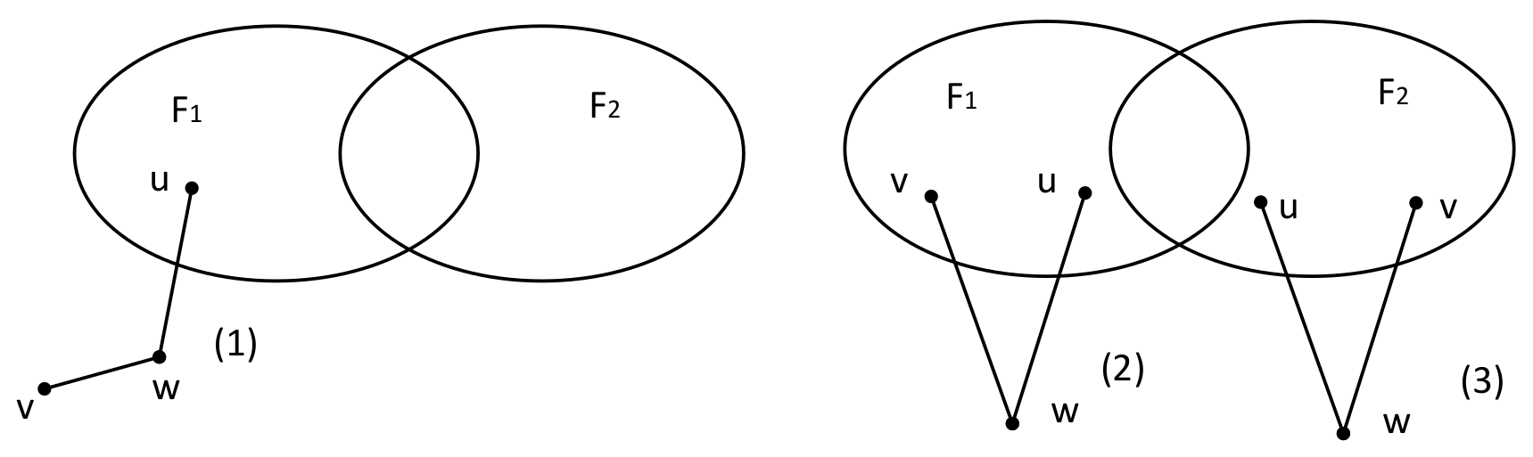
Given a simple graph G, $V\left(G\right)$ and $E\left(G\right)$ are denoted as the vertex set and the edge set, respectively. The number of vertices in G is called the order, denoted by N. An edge with end vertices u and v is denoted by $(u,v)$. For each vertex $v\in V\left(G\right)$, if $(u,v)\in E\left(G\right)$, we say that u is a neighbor of v or u is adjacent to v. For any set S, let $\left|S\right|$ denote the number of vertices in S (resp. cardinality). The set of all the neighborhoods of v is called the neighbor set of v in G, denoted by $N_G\left(v\right)$. The vertex number of the maximal independent set in G is called the dependent number of G, denoted by $\alpha \left(G\right)$. The degree of u in G is denoted by $de{g}_G\left(u\right)$, and let $\delta \left(G\right)=min\left\{de{g}_G\left(u\right)|u\in V\left(G\right)\right\}$. The largest connected component in G is named $mc\left(G\right)$.

2.2. The MM* Model

The MM model is based upon comparison. It conducts a diagnosis by comparing the responses of processor execution testing. The set of all comparisons performed by system $G=\left(V\right(G),E(G\left)\right)$ can be inscribed as a multiple graph $M=\left(V\right(G),P)$. $V\left(G\right)$ is the set of processors in the system. P denotes the set of edges and $P={(x,y)}_z$. ${(x,y)}_z$ denotes a comparison: the comparison processor z sends the same test to the two compared processors x and y and compares their responses. Side ${(x,y)}_z\in P$ is equivalent to $(x,z)\in E$ and $(y,z)\in E$, where $x,y\in N_G\left(z\right)$.

A symptom of a system is denoted by the symbol $\sigma$, defined as the set of all comparison results in the system G. A set of all nodes are tested under a $\sigma$ faulty syndrome, then the set is called a fault set F. Two faulty sets $F_1$, $F_2$ are distinguishable if $\sigma \left(F_1\right)\cap \sigma \left(F_2\right)=\varnothing$; otherwise, they are indistinguishable. The following are sufficient conditions for two fault sets $F_1$ and $F_2$ to be distinguishable pairs under the MM* model. Let $F_1△F_2$ denote the symmetric difference between $F_1$ and $F_2$, i.e., $F_1△F_2=(F_1-F_2)\cup (F_2-F_1)$.

Lemma 1 ([24]). 

Let $G=\left(V\right(G),E(G\left)\right)$ be a multiprocessor system. For any two distinct sets $F_1$, $F_2\subseteq V\left(G\right)$, $F_1$ and $F_2$ are distinguishable under the MM* model if and only if one of the following conditions is satisfied:

(1) 

There are two vertices v, $w\in V\left(G\right)-F_1\cup F_2$, and there is a vertex $u\in F_1△F_2$ such that $(u,w)\in E\left(G\right)$ and $(v,w)\in E\left(G\right)$.

(2) 

There are two vertices u, $v\in F_1\cup F_2$, and there is a vertex $w\in V\left(G\right)-F_1\cup F_2$ such that $(u,w)\in E\left(G\right)$ and $(v,w)\in E\left(G\right)$.

(3) 

There are two vertices u, $v\in F_2\cup F_1$, and there is a vertex $w\in V\left(G\right)-F_1\cup F_2$ such that $(u,w)\in E\left(G\right)$ and $(v,w)\in E\left(G\right)$.

Figure 1 shows an illustration for Lemma 1.

Figure 1. An illustration for Lemma 1.

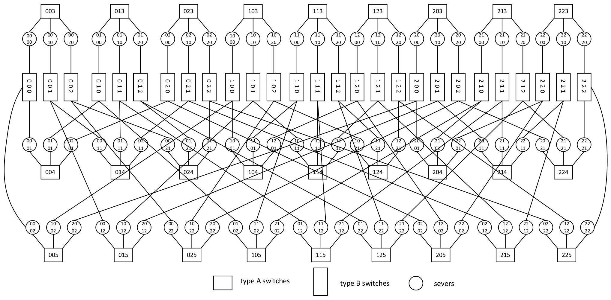
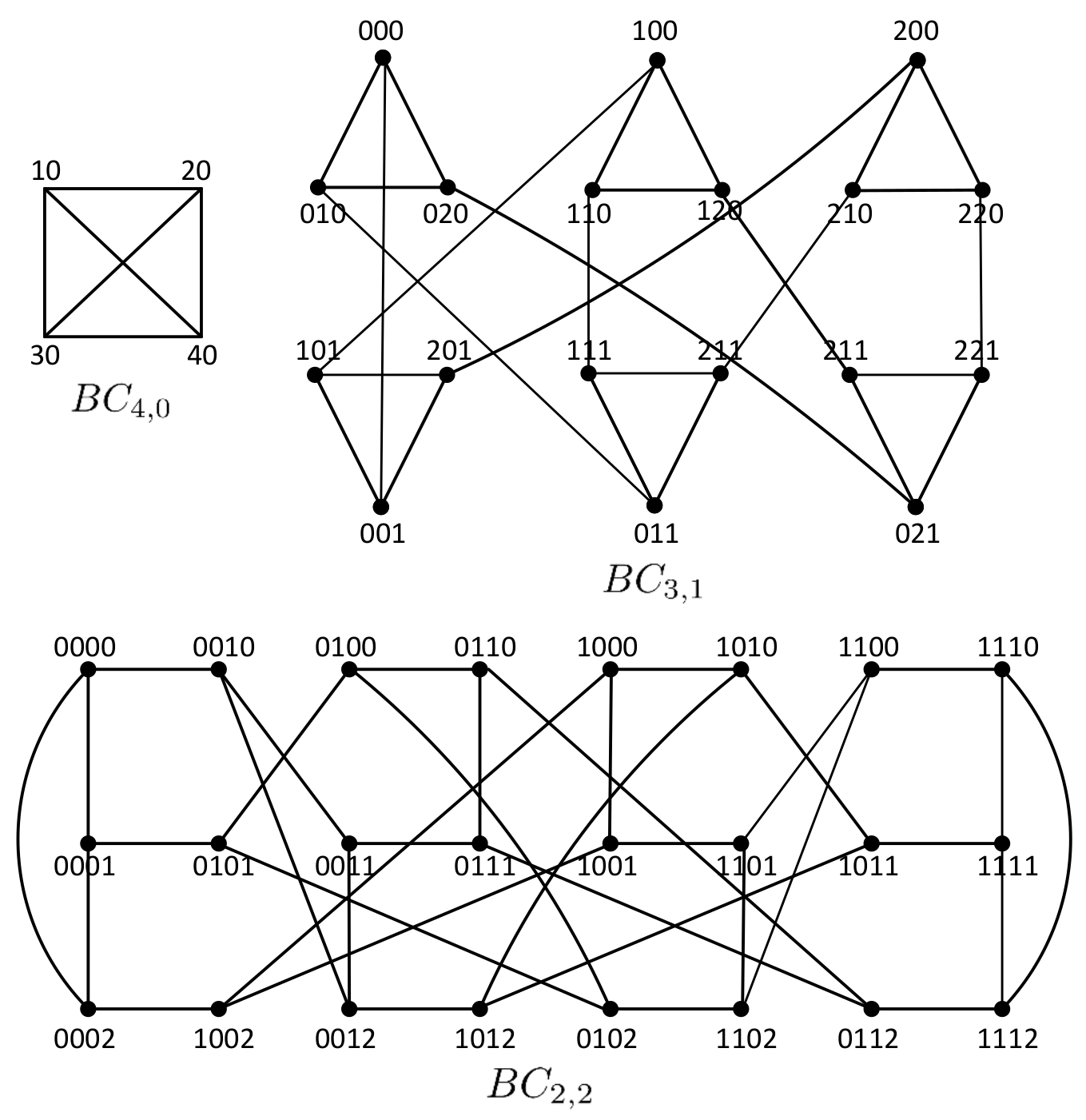
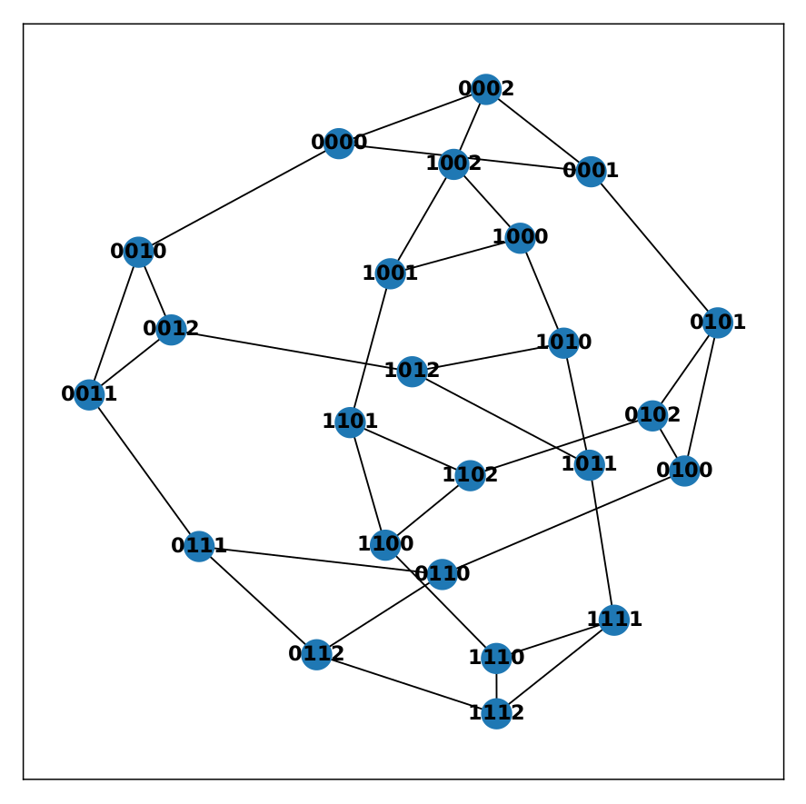
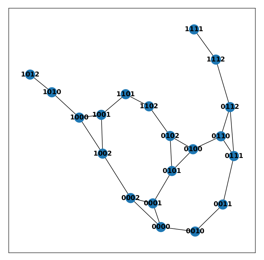
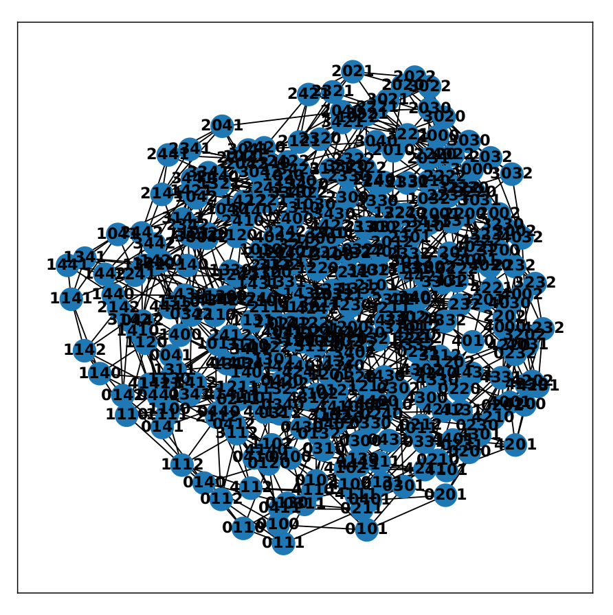
2.3. Structure and Properties of BCCC

BCCC is a structure that recursively connects servers layer by layer. In BCCC(n,k), n denotes the n-port server and k denotes the dimension. First, we let n servers connect to an n-port switch as an element, denoted by BCCC(n,0). BCCC(n,k) is composed of n BCCC(n,k-1)s connecting $n^k$ elements. Two types of switches are used in BCCC, which are type A switch and type B switch. A type A switch has n ports for forming an element, and a type B switch has $(k+1)$ ports for connecting different elements. Overall, to build BCCC(n,k), we need $(k+1)n^{k+1}$ dual-port servers, $(k+1)n^k$ type A switches and $n^{k+1}$ type B switches.

An example of BCCC(3,2) is shown in Figure 2. The study of the connectivity and diagnosability of the structure requires the equivalence of the network to a graph, which is calculated using knowledge of graph theory, where the vertices represent servers and the edges represent links. Switches are considered as transparent devices.

Figure 2. Structure of BCCC(3,2).

Definition 1. 

For any integers $k\ge 0$ and $n\ge 2$, the k-dimensional transparent BCCC network with n-port switches is denoted by a simple graph $B{C}_{n,k}=(V_{B{C}_{n,k}},E_{B{C}_{n,k}})$ with N vertices, where $V_{B{C}_{n,k}}=a_{k+1}{a}_k{a}_{k-1}...a_0$, where $a_0\in \left[0,k\right]$ and $a_i\in \left[0,n-1\right]$, $1\le i\le k+1$. Two servers $a_{k+1}{a}_k{a}_{k-1}...a_0$ and $a_{k+1}^{\prime }{a}_k^{\prime }{a}_{k-1}^{\prime }...a_0^{\prime }$ are neighbors, if and only if $\exists i$, $i=a_0+1$ or $i=0$, such that $a_i\ne a_i^{\prime }$, and $\forall j$, $0\le j\le k+1$, $i\ne j$, such that $a_j=a_j^{\prime }$. A $B{C}_{n,k}$ contains n $B{C}_{n,k-1}$ subgraphs.

Figure 3 shows three examples of $B{C}_{n,k}$s.

Figure 3. Several transparent $B{C}_{n,k}$s with small parameters n and k.

Lemma 2 ([1]). 

$B{C}_{n,k}$ has the following properties:

(1) 

$B{C}_{n,k}$ is (n+k-1)-regular graph. $N=(k+1)n^{k+1}$.

(2) 

The connectivity of $B{C}_{n,k}$ is $\kappa \left(B{C}_{n,k}\right)=n+k-1.$

(3) 

There are $n^k$ vertex-disjoint paths connecting different $B{C}_{n,k-1}$ in $B{C}_{n,k}$.

Lemma 3 ([25]). 

For any integers $n\ge 3$, $k\ge 2$ and $0\le g\le n-1$, there exists a complete graph C of order $g+1$ in $B{C}_{n,k}$ such that $\left|N_{B{C}_{n,k}}\left(V\left(C\right)\right)\right|=(g+1)(k-1)+n$, and $V\left(B{C}_{n,k}\right)-N_{B{C}_{n,k}}V\left(C\right)$ has exactly two connected components: one is V(C) and the other is $V\left(B{C}_{n,k}\right)-N_{B{C}_{n,k}}\left[V\left(C\right)\right]$, where $\delta (BCC{C}_{n,k}-N_{B{C}_{n,k}}\left[V\left(C\right)\right])\ge g$.

3. The g-Extra Connectivity of the BCCC Network

In this section, we prove the the upper and lower bounds on the g-extra connectivity separately, and finally, obtain the g-extra connectivity of the $B{C}_{n,k}$.

For any two vertices x and y in $B{C}_{n,k}$, the two numbers differ only by one digit. Let $diffp$ denote a different position from left to right. For example, $diffp(x,y)=0$ denotes the different $a_0$ number of x and y.

Lemma 4 ([1]). 

For any integers $n\ge 3$ and $k\ge 2$, let x and y be any two distinct vertices in $B{C}_{n,k}$; the two have only one digit number. Then

$$|N_{B{C}_{n,k}}\left(x\right)\cap N_{B{C}_{n,k}}\left(y\right)|\left\{\begin{array}{cc}=k-1,\hfill & \hfill ifdiffp(x,y)=0\\ =n-2,\hfill & \hfill if1\le diffp(x,y)\le k+1\\ \le 1,\hfill & \hfill if(x,y)\notin E\left(B{C}_{n,k}\right)\end{array}\right.$$

(1)

Lemma 5. 

For any integers $n\ge 3$, $k\ge 2$, $n\ge k+1$ and $0\le g\le n-1$, if $D\subseteq V\left(B{C}_{n,k}\right)$ with $\left|D\right|=g+1$, we have $\left|N_{B{C}_{n,k}}\left(D\right)\right|\ge (g+1)(k-1)+n$.

Proof. 

According to Lemma 3, when $\left|N_{B{C}_{n,k}}\left(D\right)\right|=(g+1)(k-1)+n$, $B{C}_{n,k}$ is divided into two subgraphs, each of them has least $g+1$ vertices. The lemma holds. Next, we consider that vertices are located in different connected components.

According to Lemma 1, for any two vertices u, v and $(u,v)\notin E\left(B{C}_{n,k}\right)$, they have one common neighbor at most. Similarly, for two different connected components A and B, $N_{B{C}_{n,k}}\left(A\right)\cup N_{B{C}_{n,k}}\left(B\right)\le 1$. Thus, $g+1$ vertices can be divided into $\epsilon$ disjoint vertex sets, say $D_1$,$D_2$,…,$D_{\epsilon }$. Suppose that $\left|D_i\right|=g_i$, where $2\le i\le \epsilon$, we have ${\sum }_{i=1}^{\epsilon }\left|D_i\right|=\left|D\right|=g+1$ and $\left|N_{B{C}_{n,k}}\left(D_i\right)\right|\ge g_i(k-1)+n-1$. Thus, we have

$$\begin{array}{cc}\hfill N_{B{C}_{n,k}}\left(D\right)& \ge \left|N_{B{C}_{n,k}}\left(D_1\right)\right|+\left|N_{B{C}_{n,k}}\left(D_2\right)\right|+\dots +\left|N_{B{C}_{n,k}}\left(D_{\epsilon }\right)\right|\hfill \\ \hfill & \ge \left[g_1(k-1)+n-1\right]+\left[g_2(k-1)+n-1\right]+\dots +\left[g_{\epsilon }(k-1)+n-1\right]\hfill \\ \hfill & =\sum _{1\le i\le \epsilon }\left[g_i(k-1)+n-\epsilon \right]\hfill \\ \hfill & =(g+1)(k-1)+\epsilon n-\epsilon \hfill \end{array}$$

(2)

Let $f\left(\epsilon \right)=(g+1)(k-1)+\epsilon n-\epsilon$ be a function on $\epsilon$, where $2\le \epsilon \le g+1$, it is easy to verify that $f^{\prime }\left(\epsilon \right)=n-1$. Since $n\ge 3$, we have $f^{\prime }\left(\epsilon \right)>0$. Therefore, $f^{\prime }\left(\epsilon \right)$ is an increasing function, $f\left(\epsilon \right)\ge f\left(2\right)$. We have

$$\begin{array}{cc}\hfill N_{B{C}_{n,k}}\left(D\right)& \ge (g+1)(k-1)+\epsilon n-\epsilon \hfill \\ \hfill & \ge (g+1)(k-1)+2n-2\hfill \\ \hfill & >(g+1)(k-1)+n\hfill \end{array}$$

(3)

In summary, if $D\subseteq V\left(B{C}_{n,k}\right)$ with $\left|D\right|=g+1$, we have $\left|N_{B{C}_{n,k}}\left(D\right)\right|\ge (g+1)(k-1)+n$. The lemma holds.    □

Lemma 6. 

For any integers $n\ge 3$, $k\ge 2$, $n\ge k+1$ and $0\le g\le n-1$, if $F\subseteq V\left(B{C}_{n,k}\right)$ with $\left|F\right|\le (g+1)(k-1)+n-1$, then $B{C}_{n,k}-F$ has one large component, and the remaining small components have at most g vertices in total.

Proof. 

Let $C_1$, $C_2$,…, $C_{\gamma }$, $C_{\gamma +1}$ be the components of $B{C}_{n,k}-F$, where $C_{\gamma +1}$ is the largest component. Let ${\sum }_{i=1}^{\gamma }\left|C_i\right|=\left|C\right|$. Assume that $\left|C\right|\ge g+1$. According to Lemma 5, $\left|N_{B{C}_{n,k}}\left(C\right)\right|\ge (g+1)(k-1)+n$, this is in contradiction to $\left|F\right|\le (g+1)(k-1)+n-1$. Hence, $\left|C\right|\le g$. The lemma holds.    □

Lemma 7. 

For any integers $n\ge 3$, $k\ge 2$, $n\ge k+1$ and $0\le g\le n-1$, if $F\subseteq V\left(B{C}_{n,k}\right)$ with $\left|F\right|\le (g+1)(k-1)+n-1$, then $B{C}_{n,k}-F$ has one large component at least $N-\left|F\right|-g$ vertices.

Proof. 

According to Lemma 6, $\left|C\right|\le g$ with $\left|F\right|\le (g+1)(k-1)+n-1$. We have

$$\begin{array}{cc}\hfill \left|C_{\gamma +1}\right|& =N-\left|F\right|-\left|C\right|\hfill \\ \hfill & \ge N-\left|F\right|-g\hfill \end{array}$$

(4)

Thus, the lemma holds.    □

Lemma 8. 

For any integers $n\ge 3$, $k\ge 2$, $n\ge k+1$ and $0\le g\le n-1$, the upper bound of g-extra connectivity is ${\kappa }_g\left(B{C}_{n,k}\right)\le (g+1)(k-1)+n$.

Proof. 

According to Lemma 3, when $\left|N_{B{C}_{n,k}}\left(V\left(C\right)\right)\right|=(g+1)(k-1)+n$, $V\left(B{C}_{n,k}\right)-N_{B{C}_{n,k}}V\left(C\right)$ has exactly two connected components: one is V(C) and the other is $V\left(B{C}_{n,k}\right)-N_{B{C}_{n,k}}\left[V\left(C\right)\right]$, where $\delta (BCC{C}_{n,k}-N_{B{C}_{n,k}}\left[V\left(C\right)\right])\ge g$. Meanwhile, we have $\left|C\right|=g+1$ and $|V\left(B{C}_{n,k}\right)-N_{B{C}_{n,k}}\left[V\left(C\right)\right]|=N-(g+1)-\left[(g+1)(k-1)+n\right]>g+1$. Thus, $N_{B{C}_{n,k}}\left(V\left(C\right)\right)$ is an g-extra vertex cut of $B{C}_{n,k}$. The upper bound of g-extra connectivity is ${\kappa }_g\left(B{C}_{n,k}\right)\le (g+1)(k-1)+n$.    □

Lemma 9. 

For any integers $n\ge 3$, $k\ge 2$, $n\ge k+1$ and $0\le g\le n-1$, the lower bound of g-extra connectivity is ${\kappa }_g\left(B{C}_{n,k}\right)\ge (g+1)(k-1)+n$.

Proof. 

For the sake of contradiction, suppose that F is an $R_g-$cut of $B{C}_{n,k}$ with $\left|F\right|\le (g+1)(k-1)+n-1$. By Lemma 7, $B{C}_{n,k}-N_{B{C}_{n,k}}\left(V\left(H\right)\right)$ has the largest component containing at least $N-\left|F\right|-g$ vertices, where $0\le g\le n-1$. After excluding the largest connected component, the number of remaining small connected components have the most g vertices. Hence, F is not an g-extra vertex cut of $B{C}_{n,k}$ with $\left|F\right|\le (g+1)(k-1)+n-1$, a contradiction. We have the lower bound of g-extra connectivity ${\kappa }_g\left(B{C}_{n,k}\right)\ge (g+1)(k-1)+n$.    □

According to Lemma 8 and Lemma 9, we have the following Theorem.

Theorem 1. 

For any integers $n\ge 3$, $k\ge 2$, $n\ge k+1$ and $0\le g\le n-1$, the g-extra connectivity is ${\kappa }_g\left(B{C}_{n,k}\right)=(g+1)(k-1)+n$.

4. The g-Extra Conditional Diagnosiability of the BCCC Network under the MM* Model

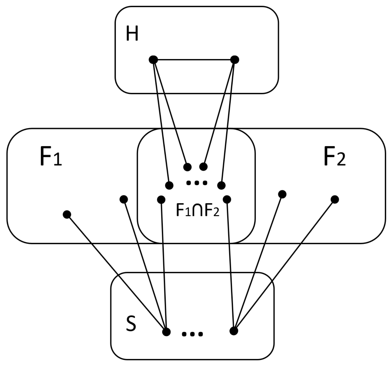
In this section, we will determine the g-extra conditional diagnosability $t_g\left(B{C}_{n,k}\right)$ of $B{C}_{n,k}$ under the MM* model for $1\le g\le n-1$.

Definition 2 ([14]). 

A simple undirected graph G = (V,E) is g-extra conditionally t-diagnosable if and only if for each pair of distinct faulty g-extra vertex sets $F_1$, $F_2\subseteq V\left(G\right)$ such that $\left|F_1\right|\le t$, $\left|F_2\right|\le t$, $F_1$ and $F_2$ are distinguishable. The g-extra conditional diagnosability of G, denoted as $t_g\left(G\right)$, is the maximum value of t such that G is g-extra conditionally t-diagnosable.

Lemma 10 ([26]). 

Let G be a connected graph with order $N\ge 2{\kappa }_g\left(G\right)+2g+\alpha \left(G\right)$ and minimum degree $\delta \left(G\right)\ge 3$, where ${\kappa }_g\left(G\right)$ is the g-extra connectivity of G, $\alpha \left(G\right)$ is the independence number of G and $g\ge 0$. If G satisfies the following conditions:

(1) 

there is a connected subgraph H of G with $\left|V\right(H\left)\right|=g+1$ such that $N_G\left(H\right)$ is a minimum g-extra cut of G;

(2) 

${\kappa }_g\left(G\right)\ge g+2$, ${\kappa }_{g+1}\left(G\right)\ge {\kappa }_g\left(G\right)+g$;

(3) 

$mc(G-F)\ge N-\left|F\right|-(g+1)$ for any vertex set $F\subseteq V\left(G\right)$ with $\left|F\right|\le {\kappa }_{g+1}\left(G\right)-1$; then, $t_g\left(G\right)={\kappa }_g\left(G\right)+g$ under the MM* model.

Lemma 11. 

The vertex number of the maximal independent set $\alpha \left(B{C}_{n,k}\right)=0$ in $B{C}_{n,k}$.

Proof. 

We first prove that $V\left(B{C}_{n,k}\right)-(F_1\cup F_2)\ne \varnothing$. If $F_1\cup F_2=\varnothing$, there are no isolated vertices in the graph and $\alpha \left(B{C}_{n,k}\right)=0$. According to Lemma 10, we suppose two g-extra fault sets $F_1$ and $F_2$ exist with $\left|F_1\right|\le {\kappa }_g\left(G\right)+g=(g+1)k+n$ and $\left|F_2\right|\le {\kappa }_g\left(G\right)+g=(g+1)k+n$. Thus, $F_1$ and $F_2$ are not satisfied with any one condition in Lemma 1. Assume that $F_1\cap F_2=\varnothing$, we have $\left|V\left(B{C}_{n,k}\right)\right|-|F_1\cup F_2|\ge (k+1)n^{k+1}-2\left[(g+1)k+n\right]$. Let $f\left(g\right)=(k+1)n^{k+1}-2\left[(g+1)k+n\right]$. Since $k\ge 2$, we have $f^{\prime }\left(g\right)<0$. Therefore, $f\left(g\right)$ is a decreasing function. $f\left(g\right)\ge f(n-1)>0$. Thus, $V\left(B{C}_{n,k}\right)-F_1\cup F_2\ne \varnothing$.

Next, prove the conclusion in $V\left(B{C}_{n,k}\right)-F_1\cup F_2\ne \varnothing$. We prove that $\alpha \left(B{C}_{n,k}\right)=0$ is equivalent to proving that $V\left(B{C}_{n,k}\right)-F_1\cup F_2$ has no isolated vertices.

Suppose there is at least one isolated vertex s in $V\left(B{C}_{n,k}\right)-F_1\cup F_2$. Suppose $F_1\subset F_2$, since $F_2$ is a g-extra fault set and s is an isolated vertex; we obtain $g=0$, which contradicts $g\ge 1$. Thus, $F_1⊈F_2$. Similarly, we have $F_2⊈F_1$. Let S be a maximum independent set of $B{C}_{n,k}-F_1\cup F_2$, and let H be the induced subgraph by the vertex set $V\left(B{C}_{n,k}\right)-(F_1\cup F_2\cup S)$.

Since $F_1$ and $F_2$ are two indistinguishable g-extra fault sets of $B{C}_{n,k}$, there exists one vertex $u\in F_2-F_1$ at most, such that u is connected to w, according to Lemma 1(2). If $N_{B{C}_{n,k}}\left(s\right)\cap (F_2-F_1)=\varnothing$, then s is an isolated vertex in $B{C}_{n,k}-F_1$, which is contradictory to $g\ne 0$. Thus, there exists only one vertex u such that u and s are adjacent to each other. Similarly, we infer that there exists only one vertex $v\in F_1-F_2$ such that v is adjacent to s. According to Lemma 2(2), $\kappa \left(B{C}_{n,k}\right)=n+k-1$. We have

$$\begin{array}{cc}\hfill |F_1\cap F_2|& \ge |N_{B{C}_{n,k}}\left(s\right)\cap (F_1\cap F_2)|\hfill \\ \hfill & =\left|N_{B{C}_{n,k}}\left(s\right)\right|-|N_{B{C}_{n,k}}\left(s\right)\cap (F_1-F_2)|-|N_{B{C}_{n,k}}\left(s\right)\cap (F_2-F_1)|\hfill \\ \hfill & =n+k-1-2\hfill \\ \hfill & =n+k-3\hfill \end{array}$$

(5)

Let S be the set of all isolated vertices. Since $\left|F_2\right|=(g+1)k+n$, we have

$$\begin{array}{cc}\hfill \sum _{s\in S}\left|N_{B{C}_{n,k}\left[F_1\cap F_2\right]}\left(s\right)\right|& =\left|S\right|(n+k-3)\hfill \\ \hfill & \le \sum _{v\in F_1\cap F_2}de{g}_{B{C}_{n,k}}\left(v\right)\hfill \\ \hfill & \le |F_1\cap F_2|(n+k-1)\hfill \\ \hfill & \le (\left|F_2\right|-1)(n+k-1)\hfill \\ \hfill & =\left[(g+1)k+n-2\right](n+k-1)\hfill \end{array}$$

(6)

Thus, $\left|S\right|\le \frac{\left[(g+1)k+n-2\right](n+k-1)}{n+k-3}$, noting that $|F_1\cup F_2|=\left|F_1\right|+\left|F_2\right|-|F_1\cap F_2|\le 2{\kappa }_g\left(B{C}_{n,k}\right)+g$. Let $H=V\left(B{C}_{n,k}\right)-(F_1\cup F_2)-S$. Suppose $V\left(H\right)=\varnothing$; when $0\le g\le n-1$, we have

$$\begin{array}{cc}\hfill |F_1\cup F_2|+\left|S\right|& =\left|F_1\right|+\left|F_2\right|-|F_1\cap F_2|+\left|S\right|\hfill \\ \hfill & \le 2{\kappa }_g\left(B{C}_{n,k}\right)+g+\frac{\left[(g+1)k+n-2\right](n+k-1)}{n+k-3}\hfill \\ \hfill & <(k+1)n^{k+1}\hfill \end{array}$$

(7)

Since $\left|V\left(B{C}_{n,k}\right)\right|=(k+1)n^{k+1}$, $V\left(B{C}_{n,k}\right)-(F_1\cup F_2)-S>0$. Hence, $V\left(H\right)\ne \varnothing$.

Since $F_1$ and $F_2$ are undistinguishable, they do not comply with Lemma 1(1). Thus, for any vertex h in H, we have $N_{F_1△F_2}\left(h\right)=\varnothing$. We infer that $N_{B{C}_{n,k}}\left(H\right)\subseteq F_1\cap F_2$. Since $F_1$ is a g-extra fault set, it can be obtained that every component $J_i\in S\cup \left[F_2-(F_1\cap F_2)\right]$ has $\left|V\left(J_i\right)\right|\ge g+1$. Similarly, $F_2$ is a g-extra fault set, and every component $K_i\in S\cup \left[F_1-(F_1\cap F_2)\right]$ has $\left|V\left(K_i\right)\right|\ge g+1$. In summary, every component $G_i\in S\cup \left[F_2-(F_1\cap F_2)\right]\cup \left[F_1-(F_1\cap F_2)\right]$ has $\left|V\left(G_i\right)\right|\ge g+1$. Since $F_1$ is a g-extra fault set, we have $\left|V\left(H_i\right)\right|\ge g+1$. Therefore, $F_1\cap F_2$ is a g-extra vertex cut (see Figure 4).

Figure 4. Illustration of $F_1\cap F_2$ is a g-extra vertex cut.

Since $F_1$ and $F_2$ are two distinguishable faulty sets, $F_1⊈F_2$ and $F_2⊈F_1$, we can induce that $|F_1-F_2|\ge 1$ and $|F_2-F_1|\ge 1$. Since $F_1$ is a g-extra vertex cut and $(F_1△F_2)\cap H=\varnothing$, we have $|(F_2-F_1)\cup S|\ge g+1$. Combining this with $|F_1-F_2|\ge 1$, $|(F_2-F_1)\cup S|+|F_1-F_2|=|(F_1△F_2)\cup S|\ge g+2$. Let $s^{\prime }$ be any node in $S^{\prime }$ and $S^{\prime }=(F_1△F_2)\cup S$. Recall that the vertex set pair $(F_1,F_2)$ is not satisfied with any one condition in Lemma 1, $V\left(S^{\prime }\right)\cap V\left(H\right)=\varnothing$, we have $N_{B{C}_{n,k}}\left(s^{\prime }\right)\subseteq F_1\cup F_2$. Let $N_{B{C}_{n,k}}\left(S^{\prime }\right)=D$. Thus, $|F_1\cup F_2|\ge \left|D\right|$. According to Theorem 1, ${\kappa }_{g+1}\left(B{C}_{n,k}\right)=(g+2)(k-1)+n\ge {\kappa }_g\left(B{C}_{n,k}\right)+g$. Thus, $\left|D\right|\ge {\kappa }_g\left(B{C}_{n,k}\right)+g$. It can be obtained that $\left|F_2\right|=|F_2-F_1|+|F_1\cap F_2|\ge {\kappa }_g\left(B{C}_{n,k}\right)+g+1$, a contradicition to $\left|F_2\right|\le {\kappa }_g\left(B{C}_{n,k}\right)+g$. We can conclude that $S=\varnothing$. There are no isolated nodes in $V\left(B{C}_{n,k}\right)-F_1\cup F_2$. $\alpha \left(B{C}_{n,k}\right)=0$. The lemma holds.    □

Theorem 2. 

For any integers $n\ge 3$, $k\ge 2$, $n\ge k+1$ and $1\le g\le n-1$, the g-extra conditional diagnosability of $B{C}_{n,k}$ under the MM* model is $t_g\left(B{C}_{n,k}\right)=(g+1)k+n$.

Proof. 

According to Lemma 11, the maximal independent set $\alpha \left(B{C}_{n,k}\right)=0$. Let $f\left(g\right)=N-2{\kappa }_g\left(B{C}_{n,k}\right)-2g=(k+1)n^{k+1}-2\left[(g+1)(k-1)\right]-2n-2g$. Thus, $f^{\prime }\left(g\right)=-2k<0$ when $k\ge 2$. So, $f\left(g\right)$ is a decreasing function. $f\left(g\right)\ge f\left(1\right)\ge 0$. The graph $B{C}_{n,k}$ satisfies with $N\ge 2{\kappa }_g\left(B{C}_{n,k}\right)+2g+\alpha \left(B{C}_{n,k}\right)$ and $\delta \left(B{C}_{n,k}\right)\ge 3$ when $n\ge 3$, $k\ge 2$, $n\ge k+1$ and $1\le g\le n-1$.

According to Theorem 1, ${\kappa }_g\left(B{C}_{n,k}\right)=N_{B{C}_{n,k}}\left(H\right)$, where $\left|V\right(H\left)\right|=g+1$, satisfying condition (1) of Lemma 10. Meanwhile, since ${\kappa }_g\left(B{C}_{n,k}\right)\ge g+2$ and ${\kappa }_{g+1}\left(B{C}_{n,k}\right)\ge {\kappa }_g\left(B{C}_{n,k}\right)+g$, this satisfies condition (2) of Lemma 10. According to Lemma 7, $mc(B{C}_{n,k}-F)\ge N-\left|F\right|-(g+1)$, where $\left|F\right|\le {\kappa }_g\left(B{C}_{n,k}\right)-1\le {\kappa }_{g+1}\left(B{C}_{n,k}\right)-1$, satisfying condition (3) of Lemma 10.

Therefore, $t_g\left(B{C}_{n,k}\right)={\kappa }_g\left(B{C}_{n,k}\right)+g=(g+1)k+n$. The theorem holds.    □

5. The t/k-Diagnosability of the BCCC Network under the MM* Model

In this section, we will calculate the t/k-diagnosability of $B{C}_{n,k}$ under the MM* model for $1\le k\le n-1$. In the t/k diagnosis strategy, we represent the number of misdiagnosed nodes with k. Meanwhile, in BCCC(n,k), different dimensions are represented with k. Hence, in order to differentiate them, we replace k with h to represent the number of misdiagnosed nodes in the t/k diagnosis.

Definition 3 ([27]). 

Given a graph $G=\left(V\right(G),E(G\left)\right)$ and a syndrome σ on G produced by a faulty set, let $x\subseteq V\left(G\right)$; the 0-test subset of node x is denoted as $C_0\left(x\right)=\{c\in V\left(G\right)|\exists a\in V\left(G\right),$$\sigma {(x,a)}_c=0\}$. The 0-test subgraph of G, denoted $T_0\left(G\right)$, is a subgraph of G defined by $V\left(T_0\left(G\right)\right)\subseteq V\left(G\right)$ and $E\left(T_0\left(G\right)\right)=\left\{(x,c)\in E\left(G\right)|c\in C_0\left(x\right),x\in C_0\left(c\right)\right\}$.

Lemma 12. 

Assume a system $G=\left(V\right(G),E(G\left)\right)$ includes at most t failure nodes and symptom σ caused by failure sets in G. We come up with the following conclusions:

1. 

If for any node x, there are $y\in V\left(G\right)$ and $(x,y)\in E\left(G\right)$ that makes $x\in C_0\left(y\right)$ and $y\in C_0\left(x\right)$, then x and y share the same state (fault or fault-free).

2. 

For any random connected component $R\in T_0\left(G\right)$, all nodes

3. 

If in $T_0\left(G\right)$ the connected component R meets condition $\left|V\right(R\left)\right|\ge t+1$, then all the nodes in R are fault-free.

Proof. 

(1)

Given a proof by contradiction, suppose that node x is faulty and y is fault-free. Select a node $z\in N_G\left(x\right)$ and $z\ne y$, then $\sigma {(y,z)}_x\ne 0$. Based on the MM* model, we have $y\notin C_0\left(x\right)$; then, there is a contradiction.

(2)

When $\left|V\right(R\left)\right|=1$, the result clearly holds. Next, we consider the situation of $\left|V\right(R\left)\right|\ge 2$. Let $x\in V\left(R\right)$ and for any $y\in N_R\left(x\right)$. It can be obtained that $y\in C_0\left(x\right)$ and $x\in C_0\left(y\right)$. According to Conclusion 1 of this Lemma, x and y share the same state. In other words, in $N_R\left(x\right)$, all the nodes share the same state as x. Similarly, all nodes in R share the same state. That is to say, all nodes in R are faulty, or all nodes in R are fault-free.

(3)

Since system G contains at most t fault nodes, it follows from the conclusion 2 of this Lemma that all nodes in R have the same state. Assuming that all nodes in R are faulty, then $\left|V\right(R\left)\right|\le t$, there is a contradiction. Then, all nodes in R are fault-free.

   □

Theorem 3. 

For any integers $n\ge 3$, $k\ge 2$, $n\ge k+1$ and $1\le h\le n-1$, $B{C}_{n,k}$ is $\left[(h+1)(k-1)+n\right]/h$-diagnosable under the MM* model.

Proof. 

Case 1: $\left|F\right|\le (h+1)(k-1)+n-1$.

According to Lemma 7, $B{C}_{n,k}-F$ has one large component S and $\left|V\right(S\left)\right|\ge N-\left|F\right|-h$. Meanwhile, $\left|V\left(S\right)\right|=mc(B{C}_{n,k}-F)=mc\left(T_0^{\prime }\left(B{C}_{n,k}\right)\right)$. Thus, we have

$$\begin{array}{cc}\hfill \left|V\right(S\left)\right|& =mc(B{C}_{n,k}-F)\hfill \\ \hfill & \ge N-\left|F\right|-h\hfill \\ \hfill & \ge N-\left[(h+1)(k-1)+n-1\right]-h\hfill \\ \hfill & \ge (k+1)n^{k+1}-\left[(h+1)(k-1)+n-1\right]-h\hfill \\ \hfill & \ge (k+1)n^{k+1}-n(k+1)+2\hfill \\ \hfill & >\left|F\right|\hfill \end{array}$$

(8)

According to Lemma 12, all nodes in S are fault free where $\left|V\right(S\left)\right|\ge \left|F\right|$. Then,

$$\begin{array}{cc}\hfill \left|F^{\prime }\right|& =N-\left|V\right(S\left)\right|\hfill \\ \hfill & \le N-(N-|F|-h)\hfill \\ \hfill & =\left|F\right|+h\hfill \end{array}$$

(9)

$F^{\prime }$ contains at most h fault-free nodes.

Case 2: $\left|F\right|=(h+1)(k-1)+n$.

Let H be a set of suspicious nodes and $H\subseteq F^{\prime }$. Therefore, $N_{B{C}_{n,k}}\left(H\right)\subseteq F$. If $\left|H\right|\le h$, $\left|F^{\prime }\right|=\left|F\right|+h$, the theorem holds. Then, we consider that $\left|H\right|\ge h+1$.

If $\left|H\right|\ge h+1$, we need to prove $\left|N_{B{C}_{n,k}}\left(H\right)\right|\ge t$. Suppose that $\left|N_{B{C}_{n,k}}\left(H\right)\right|\le t-1$. According to Lemma 6, the remaining small components C have the most h vertices in total and $\left|H\right|\le h$. This is in contradiction to $\left|H\right|\ge h+1$. By Lemma 5, $N_{B{C}_{n,k}}\left(H\right)\ge (h+1)(k-1)+n$ and $H\cap F=\varnothing$. According to a t/h diagnosis, there are mostly $(h+1)(k-1)+n$ fault nodes. Obviously, all nodes in H are fault-free, and no nodes were misdiagnosed.

In summary, $B{C}_{n,k}$ is $\left[(h+1)(k-1)+n\right]/h$-diagnosable under the MM* model.    □

6. A Fault Diagnosis Algorithm

In this section, we propose a t/k diagnosis algorithm and calculate the time complexity of the algorithm. Then, two examples are given to illustrate the implementation process of the algorithm. Finally, we analyzed the experimental results.

6.1. Formal Description of the t/k Diagnosis Algorithm under the MM* Model

According to Lemma 8, we obtain important information that there exists a largest component with at least $N-\left|F\right|-h$ with $\left|F\right|\le (h+1)(k-1)+n-1$. Meanwhile, $B{C}_{n,k}$ is $\left[(h+1)(k-1)+n\right]/h$-diagnosable under the MM* model. The algorithm can correctly diagnose all faulty nodes, provided that the upper bound on the number of faulty nodes are $(h+1)(k-1)+n$, which contains most h fault-free nodes that are misdiagnosed as faulty nodes.

The algorithm t/h-Diag first repeatedly calls algorithm C-UC(u) choosing the largest connected component. When the case appears that $\left|F\right|\le (h+1)(k-1)+n$ and $\left|U\right|>0$, UDiag(C,UC,U) is called. t/h-Diag will output C,UC,U. The C set is fault-free, UC are faulty and U is undetermined. Algorithm t/h-Diag is shown in Algorithm 1.

Algorithm 1 t/h-Diag

Input: A syndrome $\sigma$ on $B{C}_{n,k}$ produced by a faulty node set $F\subset V\left(B{C}_{n,k}\right)$ with $\left|F\right|\le (h+1)(k-1)+n$, where $n\ge 3$, $k\ge 2$, $n\ge k+1$ and $1\le h\le n-1$.

Output: C,UC,U.

1: $U\leftarrow \varphi$, $C_1\leftarrow \varphi$, $R\leftarrow V\left(B{C}_{n,k}\right)$

2: while $R\ne \varphi$do

3:      choose a node u in R, call algorithm C-UC(u) and return C,UC

4:      if $\left|C\right|>\left|F\right|$ and $\left|C\right|>\left|C_1\right|$ then

5:           $C_1\leftarrow \varphi$, $C_1\leftarrow C_1\cup C$

6:           $U{C}_1\leftarrow \varphi$, $U{C}_1\leftarrow U{C}_1\cup UC$

7:      $R\leftarrow R-u$

8: $C\leftarrow \varphi$, $C\leftarrow C\cup C_1$

9: $UC\leftarrow \varphi$, $UC\leftarrow UC\cup U{C}_1$

10: identify all nodes in C as fault-free

11: identify all nodes in UC as faulty

12: $U\leftarrow V\left(B{C}_{n,k}\right)-C-UC$

13: if $\left|U\right|>h$ then

14:      identify all nodes in U as fault-free

15: if $\left|UC\right|=t-1$ and $\left|U\right|>0$ then

16:      call algorithm UDiag(C,UC,U) and return C,UC,U

17: return C,UC,U

Algorithm C-UC(u) uses breadth-first search (BFS) to traverse from the selected node, using the Q.push() and Q.pop() operations. If u is fault-free, then the C set is all fault-free nodes and the UC set is all faulty nodes. If u is faulty, then the C set is full of faulty nodes and the UC set is full of fault-free nodes. Algorithm C-UC(u) is shown in Algorithm 2.

Algorithm 2 C-UC(u)

Input: A node $u\in V\left(B{C}_{n,k}\right)$ and a syndrome $\sigma$ on $B{C}_{n,k}$.

Output: C,UC.

1: C $\leftarrow \varphi$, UC $\leftarrow \varphi$, Q is empty

2: C $\leftarrow \left\{u\right\}$, Q.push(u)

3: label all nodes with “unvisited”

4: while len(Q)>0 do

5:      y = Q.pop(0)

6:      for each unvisited node x in $N_{B{C}_{n,k}}\left(y\right)$ do

7:            for each node z in $N_{B{C}_{n,k}}\left(x\right)$ do

8:               if $\sigma {(y,z)}_x=0$ then

9:                    Q.push(x)

10:                   C $\leftarrow C\cup \left\{x\right\}$ and label x with “visited”

11:              else

12:                    UC $\leftarrow UC\cup \left\{x\right\}$

13: return C,UC

For $\left|F\right|=(h+1)(k-1)+n-1$, when $\left|U\right|>0$, UDiag is called. Since $\left|F\right|=(h+1)(k-1)+n-1$, U has at most one fault node. Select one node in the U set to test the other two nodes; if the symptom is 1, this indicates that one of the three nodes is a faulty node. At this point, the U set is a fault-free node, except for these three nodes. Select a node to test two of the three nodes, and if the symptom is 0, the two nodes being tested are fault-free. Then, the remaining node is the faulty node. With the exception of this fault node, all nodes in U are fault-free and all nodes are tested out. Algorithm UDiag(C,UC,U) is shown in Algorithm 3.

Algorithm 3 UDiag(C,UC,U)

Input: C,UC,U and a syndrome $\sigma$ on $B{C}_{n,k}$.

Output: C,UC,U.

1: For any node $u\in U$ such that $\sigma {(v,w)}_u=1$, where $\left\{v,w\right\}\in N_U\left(u\right)$.

2: if $\sigma {(v,w)}_x=0$, where $x\in (N_U\left(v\right)-\left\{u\right\})\cup (N_U\left(w\right)-\left\{u\right\})$ then

3:  $UC\leftarrow UC\cup u$, $U\leftarrow U-u$

4: if $\sigma {(u,w)}_x=0$, where $x\in (N_U\left(u\right)-\left\{v,w\right\})\cup (N_U\left(w\right)-\left\{u\right\})$ then

5:  $UC\leftarrow UC\cup v$, $U\leftarrow U-v$

6: if $\sigma {(u,v)}_x=0$, where $x\in (N_U\left(u\right)-\left\{v,w\right\})\cup (N_U\left(w\right)-\left\{u\right\})$ then

7:  $UC\leftarrow UC\cup w$, $U\leftarrow U-w$

8: $C\leftarrow C\cup U$, $U\leftarrow \varphi$

9: return C,UC,U.

Theorem 4. 

For any integers $n\ge 3$, $k\ge 2$, $n\ge k+1$ and $0\le h\le n-1$, the time complexity of algorithm t/h-Diag is $O\left(N\right(n+k-1\left)\right)$, where N is the total number of nodes in $B{C}_{n,k}$.

Proof. 

In the algorithm t/h-Diag, the largest connected component is first obtained by calling the C-UC(u) algorithm N times each time the C-UC(u) algorithm traverses all the neighbours of node u, that is, (n+k-1) times. Therefore, the Nth C-UC(u) algorithm has the most $O\left(N\right(n+k-1\left)\right)$ time. Next, the time complexity of the algorithm UDiag(C,UC,U) is O ($2\left|U\right|$). The other steps of t/h-Diag algorithm takes at most O(N) time. Therefore, the total time complexity of the algorithm t/h-Diag is $O\left(N\right(n+k-1)+2|U|+N)=O\left(N\right(n+k-1\left)\right)$. □

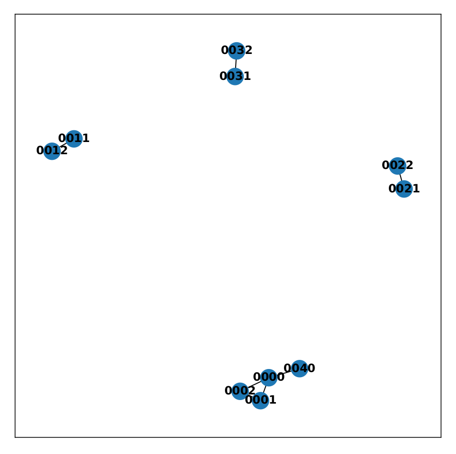
6.2. Application Example

Example 1. 

Given the network $B{C}_{2,2}$ (see Figure 5), first execute the C-UC(u) algorithm. Based on $\left|F\right|\le (h+1)(k-1)+n$, the algorithm randomly generates four faulty nodes, including 1110, 1100, 0012 and 1011. When the algorithm executes Nth times, the largest connected component is chosen to start from the node 0000. Breadth-first Search is used to put it in the set C. The largest connected component is shown in Figure 6. C = 0000, 0001, 0002, 0010, 0101, 1002, 0011, 0100, 0102, 1000, 1001, 0111, 0110, 1102, 1010, 1101, 0112, 1012, 1112, 1111. Meanwhile, UC = 1110, 1100, 0012, 1011. So, all faulty nodes have been diagnosed. There are no undiagnosed nodes.

Figure 5. $B{C}_{2,2}$ structure.

Figure 6. Largest connected component in $B{C}_{2,2}$.

Example 2. 

Given the network $B{C}_{5,2}$, we let $h=4$, at which point $\left|F\right|=(h+1)(k-1)+n=10$. The selected fault nodes are 0000, 0001, 0011, 0002, 0012, 0021, 0031, 0022, 0032, 0040. Figure 7 shows the largest connected component obtained after the breadth-first search. Figure 8 shows the faulty nodes from the breadth-first search. It can be obtained that all the faulty nodes are tested except 0000. At this point, it satisfies $\left|F\right|=(h+1)(k-1)+n-1$ and $\left|U\right|>0$. After calling the UDiag(C,UC,U) algorithm, 0000 is diagnosed as the faulty node (Figure 9 shows the set of fault nodes). So, all faulty nodes have been diagnosed. There are no undiagnosed nodes.

Figure 7. Largest connected component in $B{C}_{5,2}$.

Figure 8. Fault nodes obtained after BFS.

Figure 9. Fault nodes obtained after calling the UDiag algorithm.

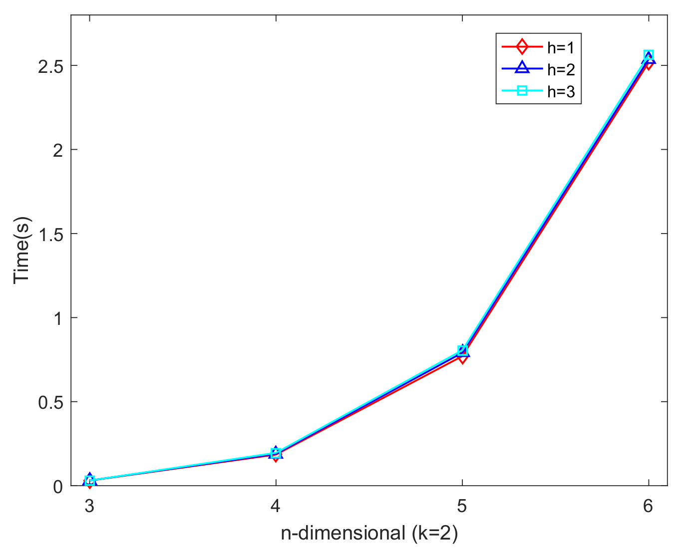
6.3. Experiments’ Results Analysis

Next, we give experimental results for the execution of the t/h-Diag algorithm. Simulation experiments were performed on computers with Intel Core i7-11800H, 2.3 GHz, 16 GB DRAM, 64 bit Windows and x64 processor. The programming language was Python. Let $B{C}_{n,k}$ be the target network, with $k=2$, $3\le n\le 7$ and $1\le h\le 3$. In addition, we randomly selected $(h+1)(k-1)+n$ faulty nodes in $B{C}_{n,k}$ by executing the algorithm 500 times and then calculating the single average time.

Figure 10 gives the average execution time of the t/h-Diag algorithm in the simulation experiments. We chose $k=2$ and $3\le n\le 6$. The three lines show the average execution time for $h=1,2,3$, respectively. It can be seen that the average execution time increases when more normal nodes are allowed to be faulty nodes and the simulation results are consistent with the time complexity of the t/h-Diag algorithm. According to the results of simulation, the execution time of the algorithm and $n^{k+1}$ are directly proportional because the time complexity of the t/h-Diag algorithm is $O\left(N\right(n+k-1\left)\right)$ and $N=(k+1)n^{k+1}$.

Figure 10. The average execution cost of the t/h-Diag algorithm.

Table 1 summarizes the number of fault nodes diagnosed by the t/h-Diag algorithm in simulation experiments. It can be seen that the algorithm can effectively diagnose all the faulty nodes. This demonstrates the accuracy and effectiveness of our algorithms. Table 2 shows one of the experimental results of 500 simulation experiments of the algorithm. The order of the faulty nodes is the order in which the algorithm obtains them.

Table 1. Number of fault nodes executing algorithm t/h-diag diagnosis.

		${\mathit{BC}}_{3,2}$	${\mathit{BC}}_{4,2}$	${\mathit{BC}}_{4,3}$	${\mathit{BC}}_{5,3}$	${\mathit{BC}}_{5,4}$
h = 1	Number of fault nodes	5	6	8	9	11
	Number of fault nodes diagnosed	5	6	8	9	11
h = 2	Number of fault nodes	6	7	10	11	14
	Number of fault nodes diagnosed	6	7	10	11	14
h = 3	Number of fault nodes	7	8	12	13	17
	Number of fault nodes diagnosed	7	8	12	13	17

Table 2. The experimental results obtained by executing the t/h-diag algorithm.

		Randomly Generated Fault Nodes	Fault Node Diagnosed
$B{C}_{3,2}$	h = 1	0202, 1112, 2021, 1101, 2211	0202, 1101, 2021, 1112, 2211
	h = 2	0211, 2011, 0121, 2120, 0212, 0120	0211, 0121, 0120, 2011, 0212, 2120
$B{C}_{4,2}$	h = 1	0210, 0331, 1032, 0312, 1110, 2032	0331, 1032, 2032, 0210, 0312, 1110
	h = 2	0012, 1230, 3312, 2231, 2331, 0131, 3202	0012, 0131, 3202, 3312, 2231, 2331, 2130
	h = 3	1321, 3200, 0210, 0130, 2320, 1211, 1000, 0100	0100, 1000, 0210, 0130, 3200, 1211, 1321, 2320
$B{C}_{4,3}$	h = 1	03132, 01322, 31033, 10200, 13003, 13220, 32322, 30210	13003, 10200, 01322, 03132, 31033, 30210, 32322, 13220

7. Conclusions

The diagnosability is the maximum number of fault processors that the system can guarantee to be diagnosed irreplaceably. It plays an important role in measuring the reliability and fault tolerance of the network. Meanwhile, a good fault diagnosis algorithm can effectively diagnose and exclude the fault nodes in the network. In this paper, we first prove that the g-extra connectivity of $B{C}_{n,k}$ is ${\kappa }_g\left(B{C}_{n,k}\right)=(g+1)(k-1)+n$, where $0\le g\le n-1$. Next, we establish the g-extra connectivity of $B{C}_{n,k}$ under the MM* model. We obtain that $t_g\left(B{C}_{n,k}\right)=(g+1)k+n$, where $1\le g\le n-1$. Based on the results of extra connectivity and the properties of the largest connectivity component, we study the t/k-diagnosability of BCCC network equal to the g-extra connectivity under the MM* model where $1\le k\le n-1$. Furthermore, we give a t/k diagnosis algorithm, which can correctly identify all nodes except most k nodes undiagnosed under the MM* model. The time complexity of the algorithm is $\left(N\right(n+k-1\left)\right)$. Finally, we have proven the accuracy and reliability of the algorithm through experiments. So far, t/k diagnosis algorithms for most interconnection networks under the MM* model have not been studied. We hope to give you some enlightenment with our proof.

What is more, the restricted edge connectivity and g-good-neighbor local diagnosability were studied in [28,29]. These new diagnostic strategies can divide large networks into smaller networks and analyze the diagnostic degree one by one. By proposing new diagnostic algorithms based on this strategy, the entire network can be diagnosed with more faulty nodes based on the new algorithms. The local diagnosability of BCCC networks can be investigated in the future.

References

- Li, Z.; Guo, Z.; Yang, Y. BCCC: An expandable network for data centers. IEEE/ACM Trans. Netw. 2016, 24, 3740–3755. [Google Scholar] [CrossRef]
- Li, X.Y.; Lin, W.; Liu, X.; Lin, C.K.; Pai, K.J.; Chang, J.M. Completely independent spanning trees on BCCC data center networks with an application to fault-tolerant routing. IEEE Trans. Parallel Distrib. Syst. 2021, 33, 1939–1952. [Google Scholar] [CrossRef]
- He, X.; Zhang, Q.; Han, Z. The Hamiltonian of Data Center Network BCCC. In Proceedings of the 2018 IEEE 4th International Conference on Big Data Security on Cloud (BigDataSecurity), IEEE International Conference on High Performance and Smart Computing,(HPSC) and IEEE International Conference on Intelligent Data and Security (IDS), Omaha, NE, USA, 3–5 May 2018; IEEE: New Jersey, NJ, USA, 2018; pp. 147–150. [Google Scholar]
- Han, Z.; Zhang, W. A summary of the BCCC data center network topology. In Proceedings of the 2018 IEEE 4th International Conference on Big Data Security on Cloud (BigDataSecurity), IEEE International Conference on High Performance and Smart Computing,(HPSC) and IEEE International Conference on Intelligent Data and Security (IDS), Omaha, NE, USA, 3–5 May 2018; IEEE: New Jersey, NJ, USA, 2018; pp. 270–272. [Google Scholar]
- Fàbrega, J.; Fiol, M.A. On the extraconnectivity of graphs. Discret. Math. 1996, 155, 49–57. [Google Scholar] [CrossRef]
- Li, J.; Huang, Y.; Lin, L.; Yu, H.; Chen, R. The extra connectivity of enhanced hypercubes. Int. J. Parallel Emergent Distrib. Syst. 2020, 35, 91–102. [Google Scholar] [CrossRef]
- Zhang, H.; Meng, J. Faulty diagnosability and g-extra connectivity of DQcube. Int. J. Parallel Emergent Distrib. Syst. 2021, 36, 189–198. [Google Scholar] [CrossRef]
- Cheng, D. Extra Connectivity and Structure Connectivity of 2-Dimensional Torus Networks. Int. J. Found. Comput. Sci. 2022, 33, 155–173. [Google Scholar] [CrossRef]
- Wang, S.; Wang, Z.; Wang, M. The 2-extra connectivity and 2-extra diagnosability of bubble-sort star graph networks. Comput. J. 2016, 59, 1839–1856. [Google Scholar] [CrossRef]
- Wang, S.; Ma, X. The g-extra connectivity and diagnosability of crossed cubes. Appl. Math. Comput. 2018, 336, 60–66. [Google Scholar] [CrossRef]
- Gu, M.M.; Hao, R.X.; Feng, Y.Q.; Yu, A.M. The 3-extra connectivity and faulty diagnosability. Comput. J. 2018, 61, 672–686. [Google Scholar] [CrossRef]
- JMaeng, M.M. Acomparisonconnectionassignmentfor self-diagnosisofmultiprocessorsystems. In Proceedings of the 11th International Symposium on Fault-Tolerant Computing, Portland, OR, USA, 24–26 June 1981; p. r175. [Google Scholar]
- Chang, N.W.; Deng, W.H.; Hsieh, S.Y. Conditional diagnosability of (n,k)-star networks under the comparison diagnosis model. IEEE Trans. Reliab. 2014, 64, 132–143. [Google Scholar] [CrossRef]
- Zhang, S.; Yang, W. The g-extra conditional diagnosability and sequential t/k-diagnosability of hypercubes. Int. J. Comput. Math. 2016, 93, 482–497. [Google Scholar] [CrossRef]
- Liu, A.; Wang, S.; Yuan, J.; Li, J. On g-extra conditional diagnosability of hypercubes and folded hypercubes. Theor. Comput. Sci. 2017, 704, 62–73. [Google Scholar] [CrossRef]
- Wang, S.; Yang, Y. The 2-good-neighbor (2-extra) diagnosability of alternating group graph networks under the PMC model and MM* model. Appl. Math. Comput. 2017, 305, 241–250. [Google Scholar] [CrossRef]
- Zhu, Q.; Wang, X.K.; Cheng, G. Reliability evaluation of BC networks. IEEE Trans. Comput. 2012, 62, 2337–2340. [Google Scholar] [CrossRef]
- Cheng, E.; Qiu, K.; Shen, Z. The g-extra diagnosability of the generalized exchanged hypercube. Int. J. Comput. Math. Comput. Syst. Theory 2020, 5, 112–123. [Google Scholar] [CrossRef]
- Wang, X.; Huang, L.; Sun, Q.; Zhou, N.; Chen, Y.; Lin, W.; Li, K. The g-extra diagnosability of the balanced hypercube under the PMC and MM* model. J. Supercomput. 2022, 78, 6995–7015. [Google Scholar] [CrossRef]
- Somani, A.K.; Peleg, O. On diagnosability of large fault sets in regular topology-based computer systems. IEEE Trans. Comput. 1996, 45, 892–903. [Google Scholar] [CrossRef]
- Xie, Y.; Liang, J.; Yin, W.; Li, C. The properties and t/s-diagnosability of k-ary n-cube networks. J. Supercomput. 2022, 78, 7038–7057. [Google Scholar] [CrossRef]
- Liu, W. The relationship between extra connectivity and t/k-diagnosability of regular networks. J. Interconnect. Netw. 2020, 20, 2050003. [Google Scholar] [CrossRef]
- Li, X.; Fan, J.; Lin, C.K.; Cheng, B.; Jia, X. The extra connectivity, extra conditional diagnosability and t/k-diagnosability of the data center network DCell. Theor. Comput. Sci. 2019, 766, 16–29. [Google Scholar] [CrossRef]
- Sengupta, A.; Dahbura, A.T. On self-diagnosable multiprocessor systems: Diagnosis by the comparison approach. IEEE Trans. Comput. 1992, 41, 1386–1396. [Google Scholar] [CrossRef]
- Li, X.; Fan, J.; Lin, C.K.; Jia, X. Diagnosability evaluation of the data center network DCell. Comput. J. 2018, 61, 129–143. [Google Scholar] [CrossRef]
- Yuan, J.; Liu, A.; Wang, X. The relationship between the g-extra connectivity and the g-extra diagnosability of networks under the MM* model. Comput. J. 2021, 64, 921–928. [Google Scholar] [CrossRef]
- Yang, X.; Tang, Y.Y. A (4n- 9)/3 diagnosis algorithm on n-dimensional cube network. Infor. Scie. 2007, 177, 1771–1781. [Google Scholar] [CrossRef]
- Zhu, Q.; Xu, J.M.; Lv, M. Edge fault tolerance analysis of a class of interconnection networks. Appl. Math. Comput. 2006, 172, 111–121. [Google Scholar] [CrossRef]
- Yin, W.; Liang, J. The g-good-neighbor local diagnosability of a hypercube network under the PMC model. IEEE Access 2020, 8, 33998–34007. [Google Scholar] [CrossRef]
Publisher’s Note: MDPI stays neutral with regard to jurisdictional claims in published maps and institutional affiliations. |
© 2022 by the authors. Licensee MDPI, Basel, Switzerland. This article is an open access article distributed under the terms and conditions of the Creative Commons Attribution (CC BY) license (https://creativecommons.org/licenses/by/4.0/).