BCCC Disjoint Path Construction Algorithm and Fault-Tolerant Routing Algorithm under Restricted Connectivity

Abstract

Connectivity in large-scale data center networks is a critical indicator to evaluate network state. A feasible and performance-guaranteed algorithm enables us to find disjoint paths between network vertices to ensure effective data transfer and to maintain the normal operation of network in case of faulty nodes. As an important data center network, BCube Connected Crossbars (BCCC) has many excellent properties that have been widely studied. In this paper, we first propose a vertex disjoint path algorithm with the time complexity of $O\left(nk\right)$ in BCCC, where n denotes a switch connected to n servers and k denotes dimension. Then, we prove that the restricted connectivity of $BCCC\left(n,k\right)$. Finally, we present an $O\left(kn{\kappa }^1\left(G\right)\right)$ fault-free algorithm in BCCC, where ${\kappa }^1\left(G\right)$ is the restricted connectivity. This algorithm can obtain a fault-free path between any two distinct fault-free vertices under the condition that each vertex has at least one fault-free neighbor in the BCCC and a set of faulty vertices F with $\left|F\right|<{\kappa }^1\left(G\right)$.

1. Introduction

The data center network (DCN) is a critical infrastructure of cloud computing, which can provide important cloud services such as GFS [1], Bigtable [2], and Dryad [3]. A data center network is a bridge connecting large-scale servers in the data center for distributed computing. As a widely used server-centric DCN, BCCC [4] can provide good network performance using inexpensive off-the-shelf switches and commodity servers with only two network interface card (NIC) ports. BCCC has many desirable properties such as high scalability, a near-equal-length parallel path, and a small diameter. The Hamilton properties and routing algorithm of BCCC have been studied [5,6,7,8].

Server failures are normal, since there are a large number of servers in the actual network. When the network fails, how to restore normal communication should be considered first. Furthermore, whether there is a fault-free path between any two different fault-free vertices and how to construct a fault-free path using an algorithm should be also taken into account. In other words, this is a problem of fault-tolerant routing, which is also the major problem we will study in this paper.

When designing or selecting a network topology for a data center, the most fundamental consideration is the fault tolerance of the network. Fault tolerance refers to the ability to continue working in the case of a network failure. Fault tolerance is the maximum number of failed devices that the network will allow to operate normally. In this paper, fault tolerance is directly determined by the connectivity of the network. The larger the connectivity scale, the better fault-tolerant performance of the data center network. In order to overcome the shortcoming of traditional connectivity, Harary [9] introduced the concept of the restricted faulty nodes on the resulting graph. Following this trend, Esfahanian [10] proposed the concept of restricted connectivity. The restricted connectivity is the connectivity under the condition that each fault-free node has at least one fault-free neighbor.

There have been many studies on the restricted connectivity of networks. Li et al. [11] establish a universally h-restricted connectivity for a class of hypercube-based compound networks, such as hierarchical cubic network and its generalization complete cubic network. Cheng [12] studies the h-restricted connectivity of an n-dimensional balanced hypercube $B{H}_n$. Li et al. [13] investigate the h-restricted connectivity of the generalized hypercube. Liu et al. [14] prove the k-restricted edge connectivity of the data center network DCell and Lin et al. [15] establish the 3-restricted connectivity of an n-dimensional split-star network. Wang [16] shows the r-restricted connectivity of hyper Petersen graphs. Ma et al. [17] prove the restricted edge connectivity of Kronecker product graphs.

Finding disjoint paths between two vertex sets in a massively parallel system establishes secure communication paths that do not interfere with each other. Constructing multiple disjoint paths for two vertices increases the probability of constructing a fault-free path. In addition to being used to avoid congestion, speed up transmission rates, and provide alternative propagation paths, disjoint paths can also enhance the robustness of vertex failures and the ability to load balance. Wu et al. [18] propose an algorithm to give the disjoint path between any two distinct vertices in dragonfly networks. Kern [19] gives exact algorithms for disjoint paths and disjoint connected subgraphs on graphs with n vertices and m edges in H-free graphs. Hadid et al. [20] propose a self-stabilizing One-to-Many node disjoint path routing algorithm in star networks.

Fault-tolerant techniques are one of the pillar technologies of the network. At the routing algorithm level, routing fault tolerance is achieved by selecting different routing paths to bypass faulty links and nodes. Therefore, a fault-tolerant routing algorithm with good effects can be achieved by improving the traditional routing algorithm. Fault-tolerant routing algorithms for different networks have been studied. Pushparaj et al. [21] propose an algorithm for routing the packets in the case of a link fault in Mesh-of-Tree (MoT) topology. The algorithm ensures that the packets will reach their destination via the shortest possible path. Nehnouh et al. [22] introduce a new fault-tolerant routing algorithm, to tolerate permanent and transient faults in network-on-chips. Zhang et al. [23] propose a novel fault-tolerant routing algorithm for 3-ary n-cube networks based on the disjoint path with structure faults. Thuan et al. [24] propose a stochastic link-fault-tolerant routing algorithm in a folded hypercube by introducing a type of limited global information called routing probabilities. Ipek et al. [25] propose a highly adaptive fault-tolerant routing algorithm for two-dimensional network-on-chips.

In this paper, we study the vertex disjoint path construction algorithm and fault-tolerant routing algorithm under restricted connectivity in the BCCC. The major contributions are as follows:

(1)

We first propose a vertex disjoint path construction algorithm in BCCC. Time complexity is o($nk$). With this algorithm, n vertex disjoint paths can be constructed for any two vertices in the BCCC.

(2)

We prove that under the condition that each vertex has at least one fault-free neighbor in BCCC, its restricted connectivity is $2\kappa \left(G\right)-k-1$ and $2\kappa \left(G\right)-n-2$, when $n<k+1$ and $n\ge k+1$, respectively, where $\kappa \left(G\right)$ is the connectivity.

(3)

We give an $O\left(kn{\kappa }^1\left(G\right)\right)$ fault-free algorithm, where ${\kappa }^1\left(G\right)$ denotes the restricted connectivity of BCCC. This algorithm can obtain a fault-free path between any two distinct fault-free vertices under the condition that each vertex has at least one fault-free neighbor.

The rest of this paper is organized as follows: Section 2 provides the preliminaries. Section 3 proposes a vertex disjoint path construction algorithm. Section 4 discusses the restricted connectivity of BCCC. Section 5 gives a fault-free algorithm to obtain a fault-free path and an analysis of the time complexity of the algorithm. Section 6 provides the discussion and conclusions.

2. Preliminaries

2.1. Graph-Theoretic Terms

Given a simple graph G, we use $V\left(G\right)$ and $E\left(G\right)$ to denote the vertex set and the edge set, respectively. An edge with end vertices u and v is denoted by $(u,v)$. For each vertex $v\in V\left(G\right)$, if $(u,v)\in E\left(G\right)$, we say that u is a neighbor of v or u is adjacent to v. The set of all the neighbors of u is called the neighbor set of u in G, denoted by $N_G\left(u\right)$. The total number of vertices of graph G is denoted by N.

Pathway P is a sequence consisting of $(x_1,x_2,\dots ,x_n)$ with a length of n, and there is $(x_m,x_m+1)\in E\left(G\right)$ for any $0\le m\le n$. For any two different paths, $P_1$ and $P_2$, the starting and ending points are the same, named x and y, respectively. If $V\left(P_1\right)\cap V\left(P_2\right)=\left\{x,y\right\}$, then $P_1$ and $P_2$ will be vertex disjoint paths. Furthermore, if all vertices in P are fault-free, then P will be a fault-free path. If $P_1$ is a path between u and x, and $P_2$ is a path between x and v in G, then let ($P_1$,$P_2$) be a path between u and v in G. The reverse of P is $(x_n,x_{n-1},\dots ,x_1)$, denoted by $P^{-1}$.

Let $F\subset V\left(G\right)$ and F be a set of faulty vertices. For any vertex x in G, if $x\in F$, then x is faulty; otherwise, x is fault-free. The connectivity of graph G is defined as $\kappa \left(G\right)$. This is the minimum number of vertices needed to make the graph disconnected or trivial. If we specify that every vertex has at least one fault-free neighbor, we call the connectivity in this case the limited connectivity, which is defined as ${\kappa }^1\left(G\right)$.

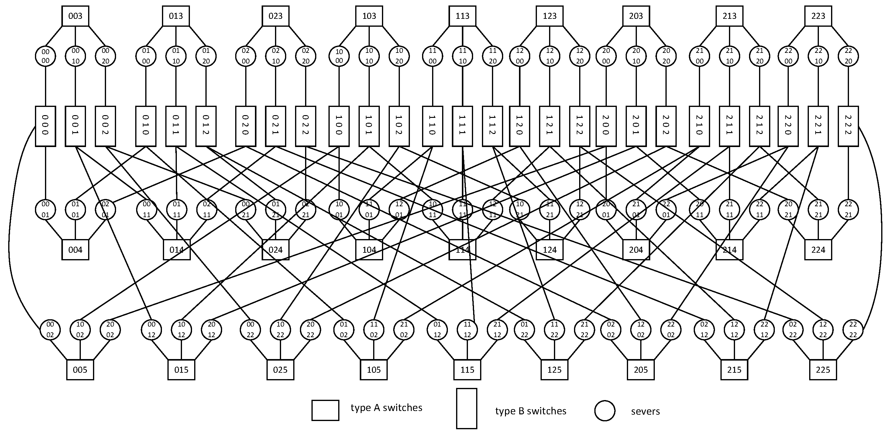
2.2. Structure and Properties of BCCC

The BCCC structure connects servers by using recursively defined squares. In $BCCC(n,k)$, n denotes the n-port server and k denotes the dimension. First, we let n servers connect to an n-port switch as an element, denoted by BCCC(n,0). BCCC(n,k) is composed of n BCCC(n,k−1)s connecting $n^k$ elements. Two types of switch are used in BCCC, which are the type A switch and type B switch. A type A switch has n ports for forming an element and a type B switch has $(k+1)$ ports for connecting different elements. Any server x in BCCC(n,k) can be represented by $x_k{x}_{k-1}\dots x_i\dots x_0,x_i\in ⟨n-1⟩$ and $i\in ⟨k⟩$. Any switch s can be represented by $s_k{s}_{k-1}\dots s_i\dots s_0$ and $s_i\in ⟨n-1⟩,1\le i\le k+1,s_0\in ⟨n+k⟩$. Overall, to build BCCC(n,k), we need $(k+1)n^{k+1}$ dual-port servers, $(k+1)n^k$ type A switches, and $n^{k+1}$ type B switches. An example of $BCCC(3,2)$ is shown in Figure 1.

Figure 1. Structure of $BCCC(3,2)$.

We can see that a pair of servers $a_{k+1}{a}_k{a}_{k-1}\dots a_0$ and $a_{k+1}^{{}^{\prime }}{a}_k^{{}^{\prime }}{a}_{k-1}^{{}^{\prime }}\dots a_0^{{}^{\prime }}$ are neighbors, meaning that they are connected by the same switch, if and only if $\exists i$, $i=a_0+1$ or $i=0$, such that $a_i\ne a_i^{{}^{\prime }}$, and $\forall j$, $0\le j\le k+1$, $i\ne j$, such that $a_j=a_j^{{}^{\prime }}$.

According to the numbering rules of the $BCCC$ server, $x_0$ connects different layers. $x_i\in \left[0,n-1\right]$, $1\le i\le k+1$. Therefore, BCCC can be divided into n subgraphs. We divide BCCC into n subgraphs according to the second digit number of the server from right to left. Servers with the same second digit number are located in the same subgraph. These subgraphs are named $BC{C}_{n,k}^1$, $BC{C}_{n,k}^2$, …, $BC{C}_{n,k}^n$. The second digit number is 0 and the subgraph is $BC{C}_{n,k}^1$. We named the server connected to other subgraphs $u_1$, and named those not connected to other subgraphs $u_2$. An example of $BCC{C}_{3,2}^1$ is shown in Figure 2.

Figure 2. Structure of $BCC{C}_{3,2}^1$.

Lemma 1.

BCCC (n,k) has the following properties [4]:

(1) 

$BCCC(n,k)$ is (n+k−1)-regular graph. $N=(k+1)n^{k+1}$.

(2) 

The connectivity of $BCCC(n,k)$ is $\kappa \left(G\right)=n+k-1.$

(3) 

There are $n^k$ vertex disjoint paths connecting different $BCCC(n,k-1)$ in $BCCC(n,k)$.

3. Vertex Disjoint Path Construction Algorithm

In this section, we propose a vertex disjoint path construction algorithm for BCCC. The algorithm constructs n vertex disjoint paths between any two nodes u and v in the BCCC.

3.1. Algorithm Description and Implementation

There are two vertex disjoint path algorithms, including BuildPathSet and Convert. BuildPathSet is the master algorithm. The Convert algorithm can change one bit of the u node number to the corresponding bit of the v node. The flow of the vertex disjoint path algorithm is as follows (refer to Algorithm 1). First, a series of v nodes located at the vertices of the same type A switch $v_2,v_1,\dots ,v_{n-1}$ are selected. Then, a vertex $v_n$ located on the same type B switch as v is determined. The mode of the first path is as follows. First, we reach node x. The value of the $u_0$ bit of x is 0. In addition, x is on the same type A switch as the source node. The path is selected from node x to node $v_1$. The second path pattern is as follows. First, some data arrive at the y node. The value of the $u_0$ bit of y is 1. In addition, node y and the source node reside on the same type A switch. The path is from node y to node $v_2$. The other paths follow the same rules. The Convert algorithm is invoked $n-1$ times during the process from the source node to the target node. One digit is changed from the highest digit of the number to the lowest digit each time.

Algorithm 1 Vertex Disjoint Path Algorithm of BCCC.

Input: Two different vertices u = $u_{k+1}{u}_k\dots u_0$ and v = $v_{k+1}{v}_k\dots v_0$ in $BCCC(n,k)$. Let the neighbor node of the same type A switch with v be $v_1,v_2,\dots ,v_{n-1}$, and select any a neighbor node in the same type B switch as $v_n$.

Output:n vertex disjoint paths from u to v.

1:  function BuildPathSet($BCCC(n,k),u,v$)

2:  $z=v$;

3:  for $i=0;i=n-1;i++$ do

4:     $v=v_{i+1}$, $Path=\varnothing$;

5:     add u to $Path$;

6:     if $u_{u0}\ne$ i then

7:        u = $u_{k+1}{u}_k\dots u_{u0}\dots u_0$, $u_{u0}$ = i, i $\in \left\{1,2,\dots ,k+1\right\}$;

8:        add u to $Path$;

9:     for j = k + 1; j > 0; j $--$ do

10:        if $u==z$ then

11:        break;

12:        if $u_j\ne v_j$ then

13:        u, $path$ = CONVERT(u, v, $u_j$, $v_j$, $Path$);

14:     if $u_0\ne v_0$ then

15:        u = $u_{k+1}{u}_k\dots v_0$;

16:        add u to $Path$;

17:     if $u\ne z$ then

18:        add v, z to $Path$;

19:     print($Path$);

20:  function CONVERT(u, v, $u_x$, $v_y$, $Path$)

21:  $u=u_{k+1}{u}_k\dots u_x\dots u_0$, x $\in \left\{1,2,\dots ,k+1\right\}$;

22:  $v=v_{k+1}{v}_k\dots v_y\dots v_0$, y $\in \left\{1,2,\dots ,k+1\right\}$;

23:  if $u_0$ == $v_0$ then

24:     $w=u$;

25:  else

26:     $u_0=v_y$;

27:     $w=u_{k+1}{u}_k\dots v_y$;

28:     add w to $Path$;

29:  $u_x=u_y$;

30:  u = $u_{k+1}{u}_k\dots v_y\dots u_0$;

31:  add u to $Path$;

32:  return(u, $Path$);

3.2. Analysis of Vertex Disjoint Path Construction Algorithm

First, the time complexity of the Convert algorithm is analyzed. The node number of u is changed from one bit to v. This node is added to the path set and the time complexity is $O\left(1\right)$. The second ’for’ loop in the BuildPathSet algorithm runs a total of k times from high to low with $O\left(k\right)$ concomitant time complexity. The first ’for’ loop causes the algorithm to form a total of n paths with $O\left(n\right)$ adjoint time complexity. In summary, the time complexity of the BuildPathSet algorithm is $O\left(nk\right)$.

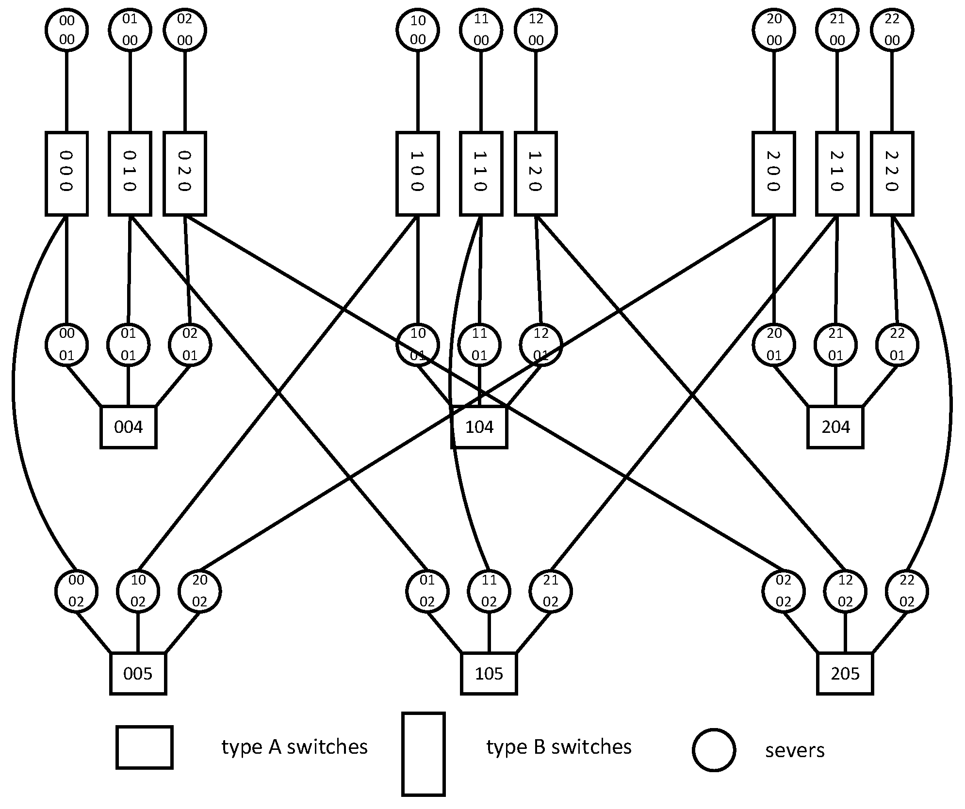
3.3. Application Examples

Example 1.

Given the network $BCCC(3,2)$ (see Figure 1), three vertex disjoint paths are constructed by the algorithm. The source node is selected as 0000 and the target node as 2011. It can be obtained that the nodes located in the same switch with the target node are 2111, 2211, and 2010. The first path is from 0000 to 2111. The Convert algorithm is used to gradually change from the highest bit to the lowest bit. Therefore, $Path1=0000\to 0002\to 2002\to 2001\to 2101\to 2100\to 2110\to 2111$. This eventually reaches 2011 through the type A switch.

The second path first selects node 0010, which is located in the same type A switch as node 0000, and reaches 2211 from 0010, using the Convert algorithm. Therefore, $Path2=0000\to 0010\to 0012\to 2012\to 2011$. Because the 2011 node is encountered on the path to the 2211 node and 2011 is the target node, the path is obtained by jumping out directly according to lines 10 and 17 of the algorithm.

The third path selects node 0020, which is located in the same type A switch as node 0000. The Convert algorithm is used to reach 2010 from 0020. Therefore, $Path3=0000\to 0020\to 0022\to 2022\to 2020\to 2010\to 2011$. Finally, three vertex disjoint paths from 0000 to 2011 are obtained.

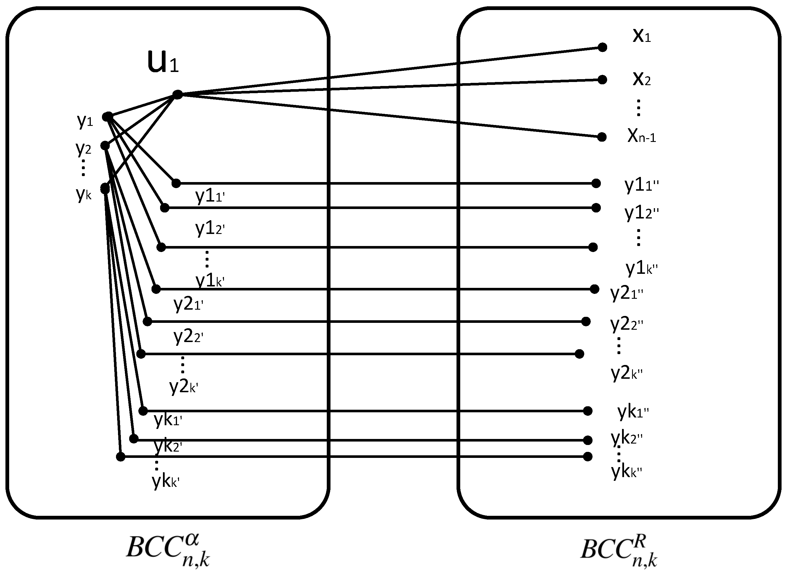
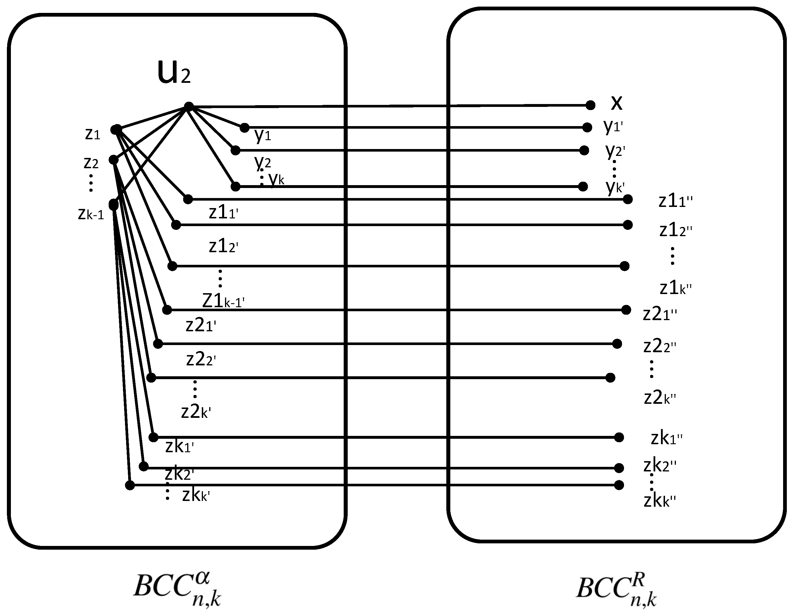
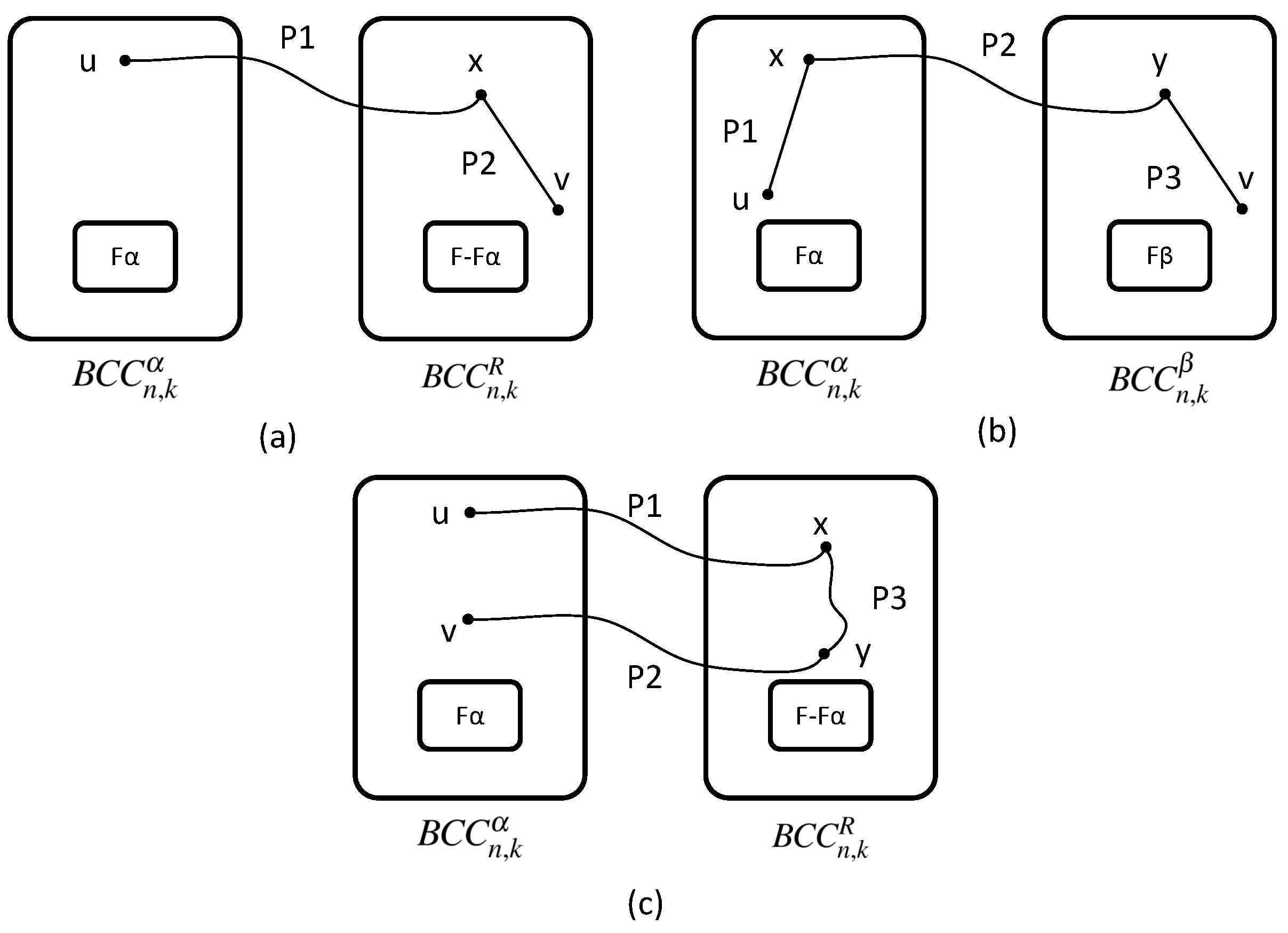
4. Restricted Connectivity of BCCC

In this section, we prove the restricted connectivity of BCCC. We refer to the entire graph of $BCCC$ as G.

Theorem 1.

The restricted connectivity of $BCCC$ is

${\kappa }^1\left(G\right)\le 2n+k-3=2\kappa \left(G\right)-k-1$, if $n<k+1$,

${\kappa }^1\left(G\right)\le n+2k-2=2\kappa \left(G\right)-n$, if $n\ge k+1$, when $n\ge 3$ and $k\ge 2$.

Proof. 

Let u and v be two vertices of the same type A switch ($v\in N_G\left(u\right)$). Therefore, $|N_G\left(u\right)\cap N_G\left(v\right)|=n-2$.

If $\left|N_G\left(u\right)\right|=\left|N_G\left(v\right)\right|=\kappa \left(G\right)$, according to the definition,

$$\begin{array}{cc}\hfill \left|N_G\left(\{u,v\}\right)\right|& =|N_G\left(u\right)\cup N_G\left(v\right)\setminus (N_G\left(u\right)\cap N_G\left(v\right))|\hfill \\ \hfill & =|N_G\left(u\right)-1|+|N_G\left(v\right)-1|-(n-2)\hfill \\ \hfill & =2\left(\kappa \right(G)-1)-(n-2)\hfill \\ \hfill & =2\kappa \left(G\right)-n\hfill \end{array}$$

(1)

Let $F=N_G\left(\left\{u,v\right\}\right)$, so $G-F$ is divided into two disconnected subgraphs: one is $G(u,v)$ and the other is $G-(N_G\left(\left\{u,v\right\}\right)\cap \left\{u,v\right\})$. Furthermore, u has a fault-free neighbor v. Therefore, each vertex of subgraph $G(u,v)$ has at least one fault-free neighbor. Let $H=N_G\left(\left\{u,v\right\}\right)\setminus \left\{u,v\right\}$, for $BCCC(n,k)$, when u and v are located in the same type A switch, each node in $N_G\left(H\right)$ has only one neighbor that is a faulty node. According to Lemma 1 (2), $\kappa \left(G\right)=n+k-1$. Therefore, $\kappa \left(G\right)$ is constantly greater than 2 when $n\ge 3$ and $k\ge 2$. It can be ensured that each node in $G-(N_G\left(\left\{u,v\right\}\right)\cap \left\{u,v\right\})$ has at least one fault-free neighbor.

In summary, $G-F$ is disconnected and each vertex in both subgraphs contains at least one fault-free neighbor. Hence, ${\kappa }^1\left(G\right)\le 2n+k-2=2\kappa \left(G\right)-n$. Therefore, the theorem holds.

Let x and y be two vertices of the same type B switch ($v\in N_G\left(u\right)$) ($y\in N_G\left(x\right)$). Therefore, $|N_G\left(x\right)\cap N_G\left(y\right)|=k-1$.

If $\left|N_G\left(x\right)\right|=\left|N_G\left(y\right)\right|=\kappa \left(G\right)$, according to the definition,

$$\begin{array}{cc}\hfill \left|N_G\left(\{x,y\}\right)\right|& =|N_G\left(x\right)\cup N_G\left(y\right)\setminus (N_G\left(x\right)\cap N_G\left(y\right))|\hfill \\ \hfill & =|N_G\left(x\right)-1|+|N_G\left(y\right)-1|-(k-1)\hfill \\ \hfill & =2\left(\kappa \right(G)-1)-(k-1)\hfill \\ \hfill & =2\kappa \left(G\right)-k-1\hfill \end{array}$$

(2)

Proving that the two vertices are in the same type B switch is the same as proving the two vertices are in the same type A switch. Let $F=N_G\left(\left\{x,y\right\}\right)$, so $G-F$ is disconnected and each vertex in both subgraphs contains at least one fault-free neighbor. Above all, ${\kappa }^1\left(G\right)\le 2k+n-3=2\kappa \left(G\right)-k-1$. Therefore, the theorem holds. □

Theorem 2.

The restricted connectivity of $BCCC$ is

${\kappa }^1\left(G\right)\ge 2n+k-3=2\kappa \left(G\right)-k-1$, if $n<k+1$,

${\kappa }^1\left(G\right)\ge n+2k-2=2\kappa \left(G\right)-n$, if $n\ge k+1$, when $n\ge 3$ and $k\ge 2$.

Proof. 

Let F be the set of faulty vertices in G. Proving this theorem is equivalent to proving, for any two vertices u and v in $G-F$, there exists a fault-free path from u to v. Furthermore, any vertex in $G-F$ has at least one fault-free neighbor.

If u and v are adjacent, the theorem holds. Hence, we discuss the case that u and v are not adjacent. According to the structure of BCCC, BCCC can be divided into n subgraphs. Let $BC{C}_{n,k}^i$ for $i\in ⟨n⟩\setminus \left\{0\right\}$ be the subgraph of G. Furthermore, $u\in BC{C}_{n,k}^{\alpha }$, $v\in BC{C}_{n,k}^{\beta }$ for $\alpha ,\beta \in ⟨n⟩\setminus \left\{0\right\}$. Let $F_{\alpha }=V\left(BC{C}_{n,k}^{\alpha }\right)\cap F$ and $F_{\beta }=V\left(BC{C}_{n,k}^{\beta }\right)\cap F$. Let $R=⟨n⟩\setminus \left\{0,\alpha \right\}$, $BC{C}_{n,k}^R$ be a subgraph other than $BC{C}_{n,k}^{\alpha }$ in G and $F_R=V\left(BC{C}_{n,k}^R\right)\cap F$. If $N_G\left(u\right)\cap V\left(BC{C}_{n,k}^R\right)\ne \varnothing$, u is named as $u_1$. Otherwise, u is named as $u_2$.

Lemma 2.

If F is a set of vertices in $BCCC(n,k)$, and for any subgraph i in $BCCC(n,k)$, $BC{C}_{n,k}^R$ is connected if $|F\cap V(G-V\left(BC{C}_{n,k}^i\right))|\le \kappa \left(G\right)-2$.

Proof. 

According to the construction rules of BCCC, U is set as the point adjacent to $BC{C}_{n,k}^i$ in $BC{C}_{n,k}^R$ to reach the conclusion that the point set of U is located in the same type A switch of subgraph $BC{C}_{n,k}^i$ and has no neighbors. Therefore, the point in the set of U points is the one with the fewest neighbors in $BC{C}_{n,k}^i$. These vertices have k vertex disjoint paths in the $BC{C}_{n,k}^i$ subgraph. This achieves $\kappa \left(BC{C}_{n,k}^i\right)=k(k\ge 2)$. Moreover, for any vertex x in $BC{C}_{n,k}^R$ to connect to $BC{C}_{n,k}^i$, one of x’s neighbors in the same type A switch is not in the subgraph. Therefore, $\kappa \left(BC{C}_{n,k}^R\right)=\kappa \left(G\right)-1$.

Because $|F\cap V(G-V\left(BC{C}_{n,k}^i\right))|\le \kappa \left(G\right)-2$ and $\kappa \left(BC{C}_{n,k}^R\right)=\kappa \left(G\right)-1$, $BC{C}_{n,k}^R$ are connected, and the Lemma holds. □

According to the position of u and v vertices in BCCC, we have the following cases.

• Case 1. $\alpha \ne \beta$.

• Subcase 1.1. $\left|F_{\alpha }\right|\ge \kappa \left(BC{C}_{n,k}^{\alpha }\right)or\left|F_{\beta }\right|\ge \kappa \left(BC{C}_{n,k}^{\beta }\right)$.

Without losing generality, suppose $\left|F_{\alpha }\right|\ge \kappa \left(BC{C}_{n,k}^{\alpha }\right)$. Apparently, $\left|F_R\right|=|F\setminus F_{\alpha }|\le 2\kappa \left(G\right)-n-1-(\kappa \left(G\right)-n+1)\le \kappa \left(G\right)-2$. According to Lemma 2, $BC{C}_{n,k}^R-F_R$ is connected. Next, we discuss the following cases.

• Subcase 1.1.1. u is $u_1$.

• Subcase 1.1.1.1. $N_G\left(u_1\right)\cap V\left(BC{C}_{n,k}^R\right)⊈F$.

Selecting a vertex x, $x\subseteq (N_G\left(u_1\right)\cap V\left(BC{C}_{n,k}^R\right))$, there is a path $P_1$ from $u_1$ to x in $BC{C}_{n,k}^{\alpha }-F_{\alpha }$. Because $BC{C}_{n,k}^R-F_R$ is connected, there exists a fault-free path $P_2$ from x to v in $BC{C}_{n,k}^R$.

• Subcase 1.1.1.2. $N_G\left(u_1\right)\cap V\left(BC{C}_{n,k}^R\right)\subseteq F$.

Because the neighbors of $u_1$ are all fault vertices in subgraph $BC{C}_{n,k}^R$, there must be a fault-free neighbor in subgraph $BC{C}_{n,k}^{\alpha }$. Now, we consider how many fault-free paths from $u_1$ to $BC{C}_{n,k}^R$ exist in $BC{C}_{n,k}^{\alpha }$. Furthermore, $N_G\left(u_1\right)\cap V\left(BC{C}_{n,k}^R\right)=n-1$.

Let $x_1,x_2,\dots ,x_{n-1}$ be all neighbors of $u_1$ in $BC{C}_{n,k}^R$.

Let $y_1,y_2,\dots ,y_k$ be all neighbors of $u_1$ in $BC{C}_{n,k}^{\alpha }$; $y_{1^{\prime }},y_{2^{\prime }},\dots ,y_{k^{\prime }}$ be the same type A switch neighbors of $y_1,y_2,\dots ,y_k$; $y_{1^{″}},y_{2^{″}},\dots ,y_{k^{″}}$ be all neighbors of $y_{1^{\prime }},y_{2^{\prime }},\dots ,y_{k^{\prime }}$ in $BC{C}_{n,k}^{\alpha }$ and $N_G\left(y_{i^{″}}\right)\cap v\left(BC{C}_{n,k}^R\right)\ne \varnothing ,i\in \left\{1,2,\dots ,k\right\}$. Thus, there are $(n-1)(k+1)$ paths from $u_1$ to $BC{C}_{n,k}^R$ as follows (refer to Figure 3). The specific paths are listed below:

$$\left\{\begin{array}{cc}\hfill X_i& =(u_1,x_i),1\le i\le n-1\hfill \\ \hfill Y_i& =(u_1,y_i,y_{i^{\prime }},y_{i^{″}}),1\le i\le k,i^{\prime }=k(n-1)\hfill \end{array}\right.$$

Figure 3. $(n-1)(k+1)$ paths from $u_1$ to $BC{C}_{n,k}^R$.

Because $N_G\left(u_1\right)\cap V\left(BC{C}_{n,k}^R\right)\subseteq F$, $F\cap V\left(BC{C}_{n,k}^R\right)\ge n-1$, $F\cap V\left(BC{C}_{n,k}^{\alpha }\right)\le {\kappa }^1\left(G\right)-1-n+1={\kappa }^1\left(G\right)-n$. Whether ${\kappa }^1\left(G\right)=2\kappa \left(G\right)-n$ or $2\kappa \left(G\right)-k-1$, $(n-1)(k+1)-k^1\left(G\right)-n\ge 1$. Therefore, there is at least one fault-free path $P_1$ from $u_1$ to $BC{C}_{n,k}^R$. Assume that t is the last vertex in the path $P_1$. If $t=v$, then $P_1$ is a path from $u_1$ to v in $G-F$. Otherwise, since $BC{C}_{n,k}^R-F_R$ is connected, there is a fault-free path $P_2$ from t to v in $BC{C}_{n,k}^R$. Then, the path $(P_1,P_2)$ is a fault-free path from $u_1$ to v in $G-F$.

• Subcase 1.1.2. u is $u_2$.

It can be obtained that $u_2$ is a vertex in $BC{C}_{n,k}^{\alpha }$ and its neighbors are all in this subgraph. According to the definition of restricted connectivity, there is a fault-free neighbor in $BC{C}_{n,k}^{\alpha }$. Now, we consider how many fault-free paths there are from $u_2$ to $BC{C}_{n,k}^R$ in $BC{C}_{n,k}^{\alpha }$.

Let x be the neighbor of $u_2$ and $N_G\left(x\right)\cap V\left(BC{C}_{n,k}^R\right)\ne \varnothing$.

Let $y_1,y_2,\dots ,y_{n-1}$ be the same type A switch neighbors of $u_2$; $y_{1^{\prime }},y_{2^{\prime }},\dots ,y_{n-1^{\prime }}$ be all neighbors of $y_1,y_2,\dots ,y_{n-1}$ in $BC{C}_{n,k}^{\alpha }$, and $N_G\left(y_{i^{\prime }}\right)\cap V\left(BC{C}_{n,k}^R\right)\ne \varnothing ,i\in \left\{1,2,\dots ,n-1\right\}$.

Let $z_1,z_2,\dots ,z_{k-1}$ be neighbors of $u_2$ in the same type B switch, except x; $z_{1^{\prime }},z_{2^{\prime }},\dots ,z_{k-1^{\prime }}$ be the same type A switch neighbors of $z_1,z_2,\dots ,z_{k-1}$; $z_{1^{″}},z_{2^{″}},\dots ,z_{k-1^{″}}$ be all neighbors of $z_{1^{\prime }},z_{2^{\prime }},\dots ,z_{k-1^{\prime }}$ in $BC{C}_{n,k}^{\alpha }$ and $N_G\left(z_{i^{″}}\right)\cap V\left(BC{C}_{n,k}^R\right)\ne \varnothing ,i\in \left\{1,2,\dots ,k-1\right\}$. Above all, there are $(k-1)(n-1)+n$ paths from $u_2$ to $BC{C}_{n,k}^R$ as follows (refer to Figure 4). The specific paths are listed below:

$$\left\{\begin{array}{cc}\hfill X_i& =(u_2,x)\hfill \\ \hfill Y_i& =(u_2,y_i,y_{i^{\prime }}),1\le i\le n-1\hfill \\ \hfill Z_i& =(u_2,z_i,z_{i^{\prime }},z_{i^{″}}),1\le i\le k-1,i^{\prime }=(k-1)(n-1)\hfill \end{array}\right.$$

Figure 4. $(k-1)(n-1)+n$ paths from $u_2$ to $BC{C}_{n,k}^R$.

Since $\left|F\right(G\left)\right|=2k\left(G\right)-n-1=2(n+k-1)-n-1=n+2k-3$, we have $(k-1)(n-1)+n-\left|F\right(G\left)\right|=1$ when $n=k+1$ and $n=3$. Furthermore, when $n>3$, whether ${\kappa }^1\left(G\right)=2\kappa \left(G\right)-n$ or $2\kappa \left(G\right)-k-1$, $(k-1)(n-1)+n-{\kappa }^1\left(G\right)>1$. Therefore, there is at least one fault-free path P in the above $(k-1)(n-1)+n$ paths from $u_2$ to $BC{C}_{n,k}^R$. Assume that w is the last vertex in the path $P_1$. If $w=v$, then $P_1$ is a path from u to v in $G-F$. Otherwise, since $BC{C}_{n,k}^R-F_R$ is connected, there is path $P_2$ between w and v in $BC{C}_{n,k}^R$. Then, the path $(P_1,P_2)$ is a path from $u_2$ to v in $G-F$.

• Subcase 1.2. $\left|F_{\alpha }\right|<\kappa \left(BC{C}_{n,k}^{\alpha }\right) \mathrm{and} \left|F_{\beta }\right|<\kappa \left(BC{C}_{n,k}^{\beta }\right)$.

Because $BC{C}_{n,k}^{\alpha }-F_{\alpha }$ and $BC{C}_{n,k}^{\beta }-F_{\beta }$ are all connected, let $\left\{x_i|x_1,x_2,\dots ,x_{n^2}\right\}$ be a set of vertices connected to other subgraphs in $BC{C}_{n,k}^{\alpha }$. Let $\left\{y_i|y_1,y_2,\dots ,y_{n^2}\right\}$ be a set of vertices connected to other subgraphs in $BC{C}_{n,k}^{\beta }$. It can be obtained that $|N_G\left(x_i\right)\cap y_i|=n^2$. Whether ${\kappa }^1\left(G\right)=2\kappa \left(G\right)-n$ or $2\kappa \left(G\right)-k-1,n^2>{\kappa }^1\left(G\right)-1$. Therefore, there must exist a fault-free vertex $x(x\in x_i)$ and $y(y\in y_i)$ in the same type A switch. If $u=x$, then it is directly connected to $BC{C}_{n,k}^{\beta }$. If $u\ne x$, since $BC{C}_{n,k}^{\alpha }-F_{\alpha }$ is connected, there exists a fault-free path $P_1$ from u to x in $BC{C}_{n,k}^{\alpha }-F_{\alpha }$. Since x and y are located in the same switch, there is a fault-free path $P_2$ from x to y. If $v=y$, it is directly connected to $BC{C}_{n,k}^{\alpha }$. If $v\ne y$, since $BC{C}_{n,k}^{\beta }-F_{\beta }$ is connected, there exists a fault-free path $p_3$ from y to v in $BC{C}_{n,k}^{\beta }-F_{\beta }$. Then, the path $(P_1,P_2,P_3)$ is a path from u to v in $G-F$ (refer to Figure 5b).

Figure 5. Figure (a) is subcase 1.1.1.1; Figure (b) is subcase 1.2; Figure (c) is subcase 2.

• Subcase 2. $\alpha =\beta$.

If $\left|F_{\alpha }\right|<\kappa \left(BC{C}_{n,k}^{\alpha }\right)$, $BC{C}_{n,k}^{\alpha }-F_{\alpha }$ is connected. There exists a fault-free path from u to v in $BC{C}_{n,k}^{\alpha }$. Thus, we only need to consider that $\left|F_{\alpha }\right|\ge \kappa \left(BC{C}_{n,k}^{\alpha }\right)$. According to subcase 1.1, if $BC{C}_{n,k}^{\alpha }-F_{\alpha }$ is not connected, $BC{C}_{n,k}^R-F_R$ is connected. According to subcase 1.1.1 and subcase 1.1.2, whether $u=u_1$ or $u=u_2$, there must exist a fault-free path from u(v) to $BC{C}_{n,k}^R$. Thus, there exists a fault-free path $P_1$ from u to a vertex x in $BC{C}_{n,k}^{\alpha }$ and a fault-free path $P_2$ from v to a vertex y in $BC{C}_{n,k}^{\alpha }$. If $x=y$, the path $(P_1,P_2^{-1})$ is a path from u to v. If $x\ne y$, since $BC{C}_{n,k}^R-F_R$ is connected, there exists a fault-free path $P_3$ from x to y. Then, the path $(P_1,P_3,P_2^{-1})$ is a path from u to v in $G-F$ (refer to Figure 5c).

In summary, if there exists a fault-free path between any two vertices u and v in BCCC, the theorem holds. □

Theorem 3.

The restricted connectivity of $BCCC$ is

${\kappa }^1\left(G\right)=n+2k-3=2\kappa \left(G\right)-k-1$, if $n<k+1$,

${\kappa }^1\left(G\right)=2n+k-2=2\kappa \left(G\right)-n$, if $n\ge k+1$, when $n\ge 3$ and $k\ge 2$.

Proof. 

According to Theorems 1 and 2, the theorem holds. □

5. Fault-Free Routing Algorithm of $\mathbf{BCCC}$ under the Restricted Connectivity

In this section, we first give a fault-free routing Algorithm $BCCFTP$. Furthermore, we analyze the time complexity of this algorithm.

5.1. Algorithm Description and Implementation

Algorithm $BCCFTP$ (refer to Algorithm 2) can give a fault-free path between any two fault-free vertices u and v in $G-F$, where F is the set of faulty vertices in G, $\left|F\right|<{\kappa }^1\left(G\right)$, and any vertex in $G-F$ has at least one neighbor.

Algorithm 2 Fault-free routing algorithm of $BCCC$.

Input: Given the graph G to represent $BCCC(n,k)$, a set of fault vertices $F\subset V\left(G\right)$, two different vertices u and v. The subgraph $\alpha$ in which u is located, subgraph $\beta$ in which v is located.

Output: A fault-free path from vertex u to v in $G-F$.

1:  function BCCFTP(u,v,$\alpha$,$\beta$,F,$BCCC(n,k)$)

2:  if $F=\varnothing$ then

3:     Return BCTP(u,v,$BCCC$,F);

4:  else if ($u,v$) $\in E\left(G\right)$ then

5:     Return(u,v);

6:  $\kappa \leftarrow \kappa$($BC{C}_{n,k}^{\alpha }$), $\alpha \leftarrow u$, $\beta \leftarrow v$;

7:  $F_{\alpha }\leftarrow F\cap (\kappa \left(BC{C}_{n,k}^{\alpha }\right)$, $F_{\beta }\leftarrow F\cap (\kappa \left(BC{C}_{n,k}^{\beta }\right)$

8:  if $\alpha \ne \beta$ then

9:     if $\left|F_{\alpha }\right|\ge \kappa$ then

10:        $P_1\leftarrow$ PATHSEQ(u, F, $BC{C}_{n,k}^{\alpha }$, $G-BC{C}_{n,k}^{\alpha }$);

11:        let s be the last vertex of $Path$ $P_1$;

12:        if $s=v$ then

13:          return $P_1$;

14:        return($P_1$, BCTP(s,v,$G-BC{C}_{n,k}^{\alpha }$, $F\setminus F_{\beta }$);

15:     else if $\left|F_{\beta }\right|\ge \kappa$ then

16:        $P_1\leftarrow$ PATHSEQ(v, F, $BC{C}_{n,k}^{\beta }$, $G-BC{C}_{n,k}^{\beta }$);

17:        let s be the last vertex of $Path$ $P_1$;

18:        if $s=u$ then

19:          return $P_1$;

20:        return(BCTP(u, s, $G-BC{C}_{n,k}^{\beta }$, F$\setminus F_{\alpha }$), $p_1^{-1}$);

21:     else $\left|F_{\alpha }\right|<\kappa$ && $\left|F_{\beta }\right|<\kappa$

22:        $P_1\leftarrow$ PATHSEQ(u, F, $BC{C}_{n,k}^{\alpha }$, $BC{C}_{n,k}^{\beta }$);

23:        let s be the last vertex of $Path$ $P_1$;

24:        if $s=v$ then

25:          return $P_1$;

26:        $P_1$+=BCTP(s, v, $BC{C}_{n,k}^{\beta }$, $F_{\beta }$);

27:        return $P_1$;

28:  else if $\left|F_{\alpha }\right|<\kappa$ then

29:     return(BCTP(u, v, $BC{C}_{n,k}^{\beta }$, $F_{\alpha }$).

30:  else

31:     $P_1\leftarrow$ PATHSEQ(u, F, $BC{C}_{n,k}^{\alpha }$, $G-BC{C}_{n,k}^{\alpha }$);

32:     let s be the last vertex of $Path$ $P_1$;

33:     $P_2\leftarrow$ PATHSEQ(v, F, $BC{C}_{n,k}^{\alpha }$, $G-BC{C}_{n,k}^{\alpha }$);

34:     let t be the last vertex of $Path$ $P_2$;

35:     if w be the first common vertex of $P_1$ and $P_2$ then

36:        return ($Path$($P_1$, u, w),$Path$($P_2^{-1}$, w, v));

37:     $P_1$+=BCTP(s, t, $G-BC{C}_{n,k}^{\alpha }$, F$\setminus F_{\alpha }$);

38:     return $P_1$+ $P_2^{-1}$;

39:

40:  function PATHSEQ(u, F, $H_1$, $H_2$)

41:  if $N_G\left(u\right)\cap V\left(H_2\right)\ne \varnothing$ then

42:     if $N_G\left(u\right)\cap V\left(H_2\right)\setminus F\ne \varnothing$ then

43:        select one fault-free vertex x from $N_G\left(u\right)\cap V\left(H_2\right)$;

44:        return(u, x);

45:     else

46:        for all $y_1\in N_G\left(u\right)\cap V\left(H_1\right)\setminus F$ do

47:          if $N_G\left(y_1\right)\cap V\left(H_1\right)\setminus F\ne \varnothing$ then

48:            for all $y_2\in N_G\left(u\right)\cap V\left(H_1\right)\setminus F$ do

49:              if $N_G\left(y_2\right)\cap V\left(H_1\right)\setminus F\ne \varnothing$ then

50:                for all $y_3\in N_G\left(u\right)\cap V\left(H_2\right)\setminus F$ do

51:                  if $N_G\left(y_3\right)\cap V\left(H_2\right)\setminus F\ne \varnothing$ then

52:                    select one fault-free vertex $y_4$ from $N_G\left(y_3\right)\cap V\left(H_2\right)\setminus F$;

53:                    return(u, $y_1$, $y_2$, $y_3$, $y_4$)

54:  else

55:     Select a vertex $x_1$ connected to other subgraphs, select a vertex $y_1$ in the same type A switch, and a vertex $z_1$ in the same type B switch from $N_G\left(u\right)\cap V\left(H_1\right)\setminus F$;

56:     if $N_G\left(x_1\right)\cap V\left(H_2\right)\setminus F\ne \varnothing$ then

57:        select one fault-free vertex $x_2$ from $N_G\left(x_1\right)\cap V\left(H_2\right)\setminus F$;

58:        return(u, $x_1$, $x_2$);

59:     if $N_G\left(y_1\right)\cap V\left(H_1\right)\setminus F\ne \varnothing$ then

60:        for all $y_2\in N_G\left(y_1\right)\cap V\left(H_1\right)\setminus F$ do

61:          if $N_G\left(y_2\right)\cap V\left(H_2\right)\setminus F\ne \varnothing$ then

62:            for all $y_3\in N_G\left(y_2\right)\cap V\left(H_2\right)\setminus F$ do

63:              select one fault-free vertex $y_3$ from $N_G\left(y_3\right)\cap V\left(H_2\right)\setminus F$;

64:              return(u, $y_1$, $y_2$, $y_3$);

65:     for all $z_2\in N_G\left(z_1\right)\cap V\left(H_1\right)\setminus F$ do

66:        if $N_G\left(z_2\right)\cap V\left(H_1\right)\setminus F\ne \varnothing$ then

67:          for all $z_3\in N_G\left(z_2\right)\cap V\left(H_1\right)\setminus F$ do

68:            if $N_G\left(z_3\right)\cap V\left(H_1\right)\setminus F\ne \varnothing$ then

69:              for all $z_4\in N_G\left(z_2\right)\cap V\left(H_2\right)\setminus F$ do

70:                select one fault-free vertex $z_4$ from $N_G\left(z_3\right)\cap V\left(H_1\right)\setminus F$;

71:                return(u, $z_1$, $z_2$, $z_3$, $z_4$);

72:

73:  function BCTP(u, v, $BCCC$, F)

74:  Select a fault free path from $BuildPathSet(BCCC,u,v)$ in $G-F$;

5.2. Analysis of Fault-Free Unicast Algorithm

First, the time complexity of $PATHSEQ(u,F,H_1,H_2)$ and $BCTP(u,v,BCC,F)$ functions is analyzed. u in $H_1$ exists in the $PATHSEQ(u,F,H_1,H_2)$ function. This depends on whether u is connected to other subgraphs, including $u_1$ and $u_2$. The path from $u_1$ to the subgraph $H_2$ is $(u,x)$, $(u,y_1,y_2,y_3,y_4)$. The time complexity of $PATHSEQ$ in different situations is as follows. First, the path is $(u,x)$, because $(N_G\left(u\right)\cap V\left(H_2\right))\setminus F\ne \varnothing$ finds a vertex x in $H_2$, and returns a path $(u,x)$. The time complexity is $O\left(1\right)$ in this case. Second, the path is $(u,y_1,y_2,y_3,y_4)$. Each vertex in the set is $y_1$ and the time complexity is $O\left(1\right)$ after traversing $(N_G\left(u\right)\cap V\left(H_1\right))\setminus F$. Each vertex in the set is $y_2$ and the time complexity is less than $O\left(\kappa \right(G\left)\right)$ after traversing $(N_G\left(y_1\right)\cap V\left(H_1\right))\setminus (F\cup u)$. Each vertex in the set is $y_3$ and the time complexity is less than $O\left(\kappa \right(G\left)\right)$ after we go through $(N_G\left(y_2\right)\cap V\left(H_1\right))\setminus (F\cup y_1)$. Each vertex in the set is $y_4$ and the time complexity is $O\left(1\right)$. After traversing $(N_G\left(y_3\right)\cap V\left(H_2\right))\setminus F$, paths $(u,y_1,y_2,y_3,y_4)$) are obtained. The time complexity is less than O$\left(\kappa {\left(G\right)}^2\right)$ in this case.

The path from $u_2$ to subgraph $H_2$ includes $(u,x_1,x_2)$, $(u,y_1,y_2,y_3)$, and $(u,z_1,z_2,z_3,z_4)$. First, the path is $(u,x_1,x_2)$. Each vertex in the set is x and the time complexity is $O\left(1\right)$ after the function traverses $(N_G\left(u\right)\cap V\left(H_1\right))\setminus F$. Next, vertex $x_2$ is found from $(N_G\left(x_1\right)\cap V\left(H_2\right))\setminus F$. The time complexity in this case is O$\left(k\right)<O\left(k\right(G\left)\right)$. Second, the path is $(u,y_1,y_2,y_3)$. The function traverses $(N_G\left(u\right)\cap V\left(H_1\right))\setminus F$. The node is set on the same type A switch as u to $y_1$ and the time complexity to $O\left(1\right)$. Then, traversing $(N_G\left(y1\right)\cap V\left(H_1\right))\setminus (F\cup u)$ sets the point connected with other subgraphs as $y_2$, and the time complexity is less than $O\left(\kappa \right(G\left)\right)$. Finally, $(N_G\left(y_2\right)\cap V\left(H_2\right))\setminus F$ is traversed and node $y_3$ selected. In this case, the time complexity is less than $O\left(\kappa \right(G\left)\right)$. Third, the path of $u_2$ $(u,z_1,z_2,z_3,z_4)$ is the same as the path of $u_1$ $(u,y_1,y_2,y_3,y_4)$. In summary, the time complexity of the $PATHSEQ(u,F,H_1,H_2)$ function is $O\left(\kappa {\left(G\right)}^2\right)$ combined with $u_1$ and $u_2$.

Next, we analyze $BCCFTP(u,v,\alpha ,\beta ,F,BCC(n,k\left)\right)$. $BCCFTP$ is divided into two cases, including $\alpha \ne \beta$ and $\alpha =\beta$.

In the case of $\alpha \ne \beta$, if $\left|F_{\alpha }\right|\ge k$, Algorithm $BCCFTP$ will first obtain a fault-free path $P_1$ from u to a vertex s in $G-BC{C}_{n,k}^{\alpha }$ by $PATHSEQ(u,F,BC{C}_{n,k}^{\alpha },G-BC{C}_{n,k}^{\alpha })$. The time complexity of this part is $O\left(\kappa {\left(G\right)}^2\right)$. Next, Algorithm $BCCFTP$ will return $P_1$ if $s=v$; then, the time to obtain the path from u to v in $G-F$ is $O\left(\kappa {\left(G\right)}^2\right)$. Otherwise, Algorithm $BCCFTP$ will return ($P_1$,$BCTP(s,v,G-BC{C}_{n,k}^{\alpha },F\setminus F_{\beta })$); then, the time to run $BCTP(s,v,G-BC{C}_{n,k}^{\alpha },F\setminus F_{\beta })$ is O$\left(kn{\kappa }^1\left(G\right)\right)$ and the time to obtain a path ($P_1$,$BCTP(s,v,G-BC{C}_{n,k}^{\alpha },F\setminus F_{\beta }))$ by connecting path $P_1$ and $BCTP$ is O$\left(1\right)$. Thus, the time to obtain the path from u to v in $G-F$ is O$(\kappa {\left(G\right)}^2+kn{\kappa }^1\left(G\right)+1)$ = O$\left(kn{\kappa }^1\left(G\right)\right)$. Furthermore, for subcases $\left|F_{\beta }\right|\ge k$, $\left|F_{\alpha }\right|<k$, and $\left|F_{\beta }\right|<k$, the time to obtain the path from u to v in $G-F$ is O$\left(kn{\kappa }^1\left(G\right)\right)$, which is similar to that discussed in the case of $\left|F_{\alpha }\right|\ge k$.

In the case of $\alpha =\beta$, if $\left|F_{\alpha }\right|\le k$, Algorithm $BCCFTP$ will firstly obtain a fault-free path from u to v in $BC{C}_{n,k}^{\alpha }$ by PATHSEQ $(u,F,BC{C}_{n,k}^{\alpha },F_{\alpha })$. The time complexity of this part is O$\left(\kappa {\left(G\right)}^2\right)$. Then, Algorithm BCCFTP will first obtain a fault-free path $P_1$ from u to a vertex s and path $P_2$ from v to a vertex t in $BC{C}_{n,k}^{\alpha }$ in the time of O$\left(\kappa {\left(G\right)}^2\right)$. If $P_1$ and $P_2$ have a common vertex w, Algorithm $BCCFTP$ will return (Path$(P_1,u,w)$, Path$(P_2^{-1},w,v))$. Since the time to obtain Path$(P_1,u,w)$ is O$\left(1\right)$, the time complexity is O$(2\ast \kappa {\left(G\right)}^2+O\left(1\right))$ = O$\left(\kappa {\left(G\right)}^2\right)$. If $P_1$ and $P_2$ have no common vertex, the function will run $BCTP(s,t,G-BC{C}_{n,k}^{\alpha },F\setminus F_{\alpha })$ to construct a fault-free path from s to t. The time complexity of this part is O$\left(kn{\kappa }^1\left(G\right)\right)$. Therefore, the time to obtain the path from u to v in G is O$(2\ast \kappa {\left(G\right)}^2+kn{\kappa }^1\left(G\right)+2\ast 1)$ = O$\left(kn{\kappa }^1\left(G\right)\right)$.

In summary, the time complexity of Algorithm $BCCFTP$ is O$\left(kn{\kappa }^1\left(G\right)\right)$.

6. Discussion and Conclusions

As the infrastructure of cloud computing, data center networking has become a hot topic in recent years. As an important DCN model, BCCC can support millions of servers with excellent communication characteristics and provide good fault tolerance. In this paper, a point disjoint path algorithm with time complexity $O\left(nk\right)$ is proposed. The algorithm can give n vertex disjoint paths between any two vertices. Multiple disjoint paths can enhance routing performance and improve network reliability. Then, we prove the condition that each vertex has at least one fault-free neighbor, and that the restricted connectivity of BCCC is $2\kappa \left(G\right)-k-1$ and $2\kappa \left(G\right)-n$, when $n<k+1$ and $n\ge k+1$, respectively. Restricted connectivity can be obtained at almost twice the traditional connectivity. The larger the connectivity scale, the better the fault-tolerant performance of the data center network. Finally, we give the $O\left(kn{\kappa }^1\left(G\right)\right)$ trouble-free algorithm with limited connectivity. This algorithm can obtain the fault-free path between any two different fault-free vertices. The premise is that each vertex has at least one fault-free neighbor in the BCCC.

Our algorithm is proposed based on the condition that each fault-free vertex has one fault-free neighbor. In the majority of cases, each vertex has more than one fault-free neighbor in large interconnected networks. In the future, the h-restricted connectivity $(h\ge 2)$ of BCCC will be studied, which is a guarantee for accommodating more failed servers when the network is large enough. Fault-free algorithms based on h-restricted connectivity can ensure that the network allows more fault nodes. In addition, many other network connectivity limitations in DCN have not been studied, such as Ficonn [26], HCN and BCN [27]. This, together with the design of related routing algorithms, may be worth further investigation. In the meantime, most networks only consider server failures. In fact, both switches and links could fail. There are currently few studies on switch and link failures. Therefore, the fault tolerance of switches and links in the network can be analyzed, and corresponding fault-tolerant routing algorithms can be designed to ensure the connectivity of the network.

References

1. Ghemawat, S.; Gobioff, H.; Leung, S.T. The Google file system. In Proceedings of the Nineteenth ACM Symposium on Operating Systems Principles, Bolton Landing, NY, USA, 19–22 October 2003; pp. 29–43. [Google Scholar]
2. Chang, F.; Dean, J.; Ghemawat, S.; Hsieh, W.C.; Wallach, D.A.; Burrows, M.; Chandra, T.; Fikes, A.; Gruber, R.E. Bigtable: A distributed storage system for structured data. ACM Trans. Comput. Syst. (TOCS) 2008, 26, 1–26. [Google Scholar] [CrossRef]
3. Isard, M.; Budiu, M.; Yu, Y.; Birrell, A.; Fetterly, D. Dryad: Distributed data-parallel programs from sequential building blocks. In Proceedings of the 2nd ACM SIGOPS/EuroSys European Conference on Computer Systems 2007, Lisboa, Portugal, 21–23 March 2007; pp. 59–72. [Google Scholar]
4. Li, Z.; Guo, Z.; Yang, Y. BCCC: An expandable network for data centers. In Proceedings of the Tenth ACM/IEEE Symposium on Architectures for Networking and Communications Systems, Marina del Rey, CA, USA, 20–21 October 2014; pp. 77–88. [Google Scholar]
5. Castillo, A.C. BCube Connected Crossbar and GBC3 Network Architecture: An Overview. In Proceedings of the 2022 31st Conference of Open Innovations Association (FRUCT), Helsinki, Finland, 27–29 April 2022; pp. 37–44. [Google Scholar]
6. Li, X.Y.; Lin, W.; Liu, X.; Lin, C.K.; Pai, K.J.; Chang, J.M. Completely independent spanning trees on BCCC data center networks with an application to fault-tolerant routing. IEEE Trans. Parallel Distrib. Syst. 2021, 33, 1939–1952. [Google Scholar] [CrossRef]
7. He, X.; Zhang, Q.; Han, Z. The Hamiltonian of Data Center Network BCCC. In Proceedings of the 2018 IEEE 4th International Conference on Big Data Security on Cloud (BigDataSecurity), IEEE International Conference on High Performance and Smart Computing,(HPSC) and IEEE International Conference on Intelligent Data and Security (IDS), Omaha, NE, USA, 3–5 May 2018; pp. 147–150. [Google Scholar]
8. Han, Z.; Zhang, W. A summary of the BCCC data center network topology. In Proceedings of the 2018 IEEE 4th International Conference on Big Data Security on Cloud (BigDataSecurity), IEEE International Conference on High Performance and Smart Computing, (HPSC) and IEEE International Conference on Intelligent Data and Security (IDS), Omaha, NE, USA, 3–5 May 2018; pp. 270–272. [Google Scholar]
9. Harary, F. Conditional connectivity. Networks 1983, 13, 347–357. [Google Scholar] [CrossRef]
10. Esfahanian, A.H. Generalized measures of fault tolerance with application to n-cube networks. IEEE Trans. Comput. 1989, 38, 1586–1591. [Google Scholar] [CrossRef]
11. Li, X.; Zhou, S.; Ma, T.; Guo, X.; Ren, X. The h-Restricted Connectivity of a Class of Hypercube-Based Compound Networks. Comput. J. 2022, 65, 2528–2534. [Google Scholar] [CrossRef]
12. Cheng, D. The h-restricted connectivity of balanced hypercubes. Discret. Appl. Math. 2021, 305, 133–141. [Google Scholar] [CrossRef]
13. Li, X.; Zhou, S.; Guo, X.; Ma, T. The h-restricted connectivity of the generalized hypercubes. Theor. Comput. Sci. 2021, 850, 135–147. [Google Scholar] [CrossRef]
14. Liu, X.; Meng, J. The k-restricted edge-connectivity of the data center network DCell. Appl. Math. Comput. 2021, 396, 125941. [Google Scholar] [CrossRef]
15. Lin, L.; Huang, Y.; Wang, X.; Xu, L. Restricted connectivity and good-neighbor diagnosability of split-star networks. Theor. Comput. Sci. 2020, 824, 81–91. [Google Scholar] [CrossRef]
16. Wang, S. The r-Restricted Connectivity of Hyper Petersen Graphs. IEEE Access 2019, 7, 109539–109543. [Google Scholar] [CrossRef]
17. Ma, T.; Wang, J.; Zhang, M. The restricted edge-connectivity of Kronecker product graphs. Parallel Process. Lett. 2019, 29, 1950012. [Google Scholar] [CrossRef]
18. Wu, S.; Fan, J.; Cheng, B.; Yu, J.; Wang, Y. Connectivity and constructive algorithms of disjoint paths in dragonfly networks. Theor. Comput. Sci. 2022, 922, 257–270. [Google Scholar] [CrossRef]
19. Kern, W.; Martin, B.; Paulusma, D.; Smith, S.; van Leeuwen, E.J. Disjoint paths and connected subgraphs for H-free graphs. Theor. Comput. Sci. 2022, 898, 59–68. [Google Scholar] [CrossRef]
20. Hadid, R.; Villain, V. A Self-stabilizing One-To-Many Node Disjoint Paths Routing Algorithm in Star Networks. In Proceedings of the IFIP International Conference on Distributed Applications and Interoperable Systems; Springer: Berlin/Heidelberg, Germany, 2020; pp. 186–203. [Google Scholar]
21. Pushparaj, J.; Soumya, J.; Veda Bhanu, P. A link fault tolerant routing algorithm for mesh of tree based network-on-chips. In Proceedings of the 2019 IEEE International Symposium on Smart Electronic Systems (iSES) (Formerly iNiS), Rourkela, India, 16–18 December 2019; pp. 181–184. [Google Scholar]
22. Nehnouh, C.; Senouci, M. A New Fault Tolerant Routing Algorithm for Networks on Chip. Int. J. Embed.-Real-Time Commun. Syst. (IJERTCS) 2019, 10, 68–85. [Google Scholar] [CrossRef] [Green Version]
23. Zhang, Y.; Fan, W.; Han, Z.; Song, Y.; Wang, R. Fault-tolerant routing algorithm based on disjoint paths in 3-ary n-cube networks with structure faults. J. Supercomput. 2021, 77, 13090–13114. [Google Scholar] [CrossRef]
24. Thuan, B.T.; Ngoc, L.B.; Kaneko, K. A stochastic link-fault-tolerant routing algorithm in folded hypercubes. J. Supercomput. 2018, 74, 5539–5557. [Google Scholar] [CrossRef]
25. Ipek, A.; Tosun, S.; Ozdemir, S. HAFTA: Highly adaptive fault-tolerant routing algorithm for two-dimensional network-on-chips. Concurr. Comput. Pract. Exp. 2021, 33, e6378. [Google Scholar] [CrossRef]
26. Li, D.; Guo, C.; Wu, H.; Tan, K.; Zhang, Y.; Lu, S. FiConn: Using backup port for server interconnection in data centers. In Proceedings of the IEEE INFOCOM 2009, Rio de Janeiro, Brazil, 19–25 April 2009; pp. 2276–2285. [Google Scholar]
27. Guo, D.; Chen, T.; Li, D.; Li, M.; Liu, Y.; Chen, G. Expandable and cost-effective network structures for data centers using dual-port servers. IEEE Trans. Comput. 2012, 62, 1303–1317. [Google Scholar]