Mixed Alternating Projections with Application to Hankel Low-Rank Approximation

Abstract

The method of alternating projections for extracting low-rank signals is considered. The problem of decreasing the computational costs while keeping the estimation accuracy is analyzed. The proposed algorithm consists of alternating projections on the set of low-rank matrices and the set of Hankel matrices, where iterations of weighted projections with different weights are mixed. For algorithm justification, theory related to mixed alternating projections to linear subspaces is studied and the limit of mixed projections is obtained. The proposed approach is applied to the problem of Hankel low-rank approximation for constructing a modification of the Cadzow algorithm. Numerical examples compare the accuracy and computational cost of the proposed algorithm and Cadzow iterations.

1. Introduction

Problem. Consider the problem of extracting a signal $\mathsf{S}={(s_1,\dots ,s_N)}^{\mathrm{T}}$ from a noisy time series $\mathsf{X}=\mathsf{S}+\mathsf{N}$, where $\mathsf{S}$ is governed by a linear recurrence relation (LRR) of order r: $s_n={\sum }_{i=1}^r{a}_i{s}_{n-i}$, $n=r+1,\dots ,N$, $a_r\ne 0$, $\mathsf{N}$ is noise with zero expectation and autocovariance matrix $\Sigma ={\Sigma }_N\in {\mathbb{R}}^{N\times N}$. There is a well-known result that describes the set of time series governed by LRRs in parametric form: $s_n={\sum }_i{P}_i\left(n\right)exp\left({\beta }_{i}n\right)cos(2\pi {\omega }_{i}n+{\psi }_i)$, where $P_i\left(n\right)$ are polynomials in n (see, e.g., ([1], Theorem 3.1.1)). Methods based on the estimation of signal subspace (subspace-based methods), and in particular, singular spectrum analysis (see [2,3,4]), work well for the analysis of such signals.

The subspace-based approach starts from fixing a window length L, $1<L<N$, putting $K=N-L+1$ and constructing the L-trajectory matrix for a series $\mathsf{S}\in {\mathbb{R}}^N$:

$$\mathbf{S}={\mathcal{T}}_L\left(\mathsf{S}\right)=\left(\begin{array}{cccc}{s}_1& s_2& \dots & s_K\\ s_2& s_3& \dots & s_{K+1}\\ ⋮& ⋮& ⋮& ⋮\\ s_L& s_{L+1}& \dots & s_N\end{array}\right),$$

where ${\mathcal{T}}_L$ denotes the bijection between ${\mathbb{R}}^N$ and $\mathcal{H}$; $\mathcal{H}$ is the set of Hankel matrices of size $L\times K$ with the equal values on the auxiliary diagonals $i+j=\mathrm{const}$.

We say that the time series $\mathsf{S}$ is called a time series of rank r, if its trajectory matrix $\mathbf{S}$ is rank-deficient and has rank r for any L, $r<L<N-r+1$. The equivalent definition of series of rank r, $2r<N$, is that $(r+1)$-trajectory matrix has rank r ([5], Corollary 5.1). Denote the set of time series of rank r and length N as ${\mathcal{D}}_r^N={\mathcal{D}}_r$.

Consider the problem of approximating a time series by series of rank r in a weighted Euclidean norm as the following non-linear weighted least-squares problem:

$${\mathsf{Y}}^{☆}=\underset{\mathsf{Y}\in \overline{{\mathcal{D}}_r}}{arg\; min}{\parallel \mathsf{X}-\mathsf{Y}\parallel }_{\mathbf{W}}^2,$$

(1)

where $\mathsf{X}$, $\mathsf{Y}\in {\mathbb{R}}^N$ are time series of length N and ${\parallel \mathsf{Z}\parallel }_{\mathbf{W}}$ is the weighted Euclidean norm generated by the inner product

$${\langle {\mathsf{Z}}_1,{\mathsf{Z}}_2\rangle }_{\mathbf{W}}={\mathsf{Z}}_1^{\mathrm{T}}\mathbf{W}{\mathsf{Z}}_2,$$

(2)

$\mathbf{W}\in {\mathbb{R}}^{N\times N}$ is a symmetric positive-definite weight matrix and ${\overline{\mathcal{D}}}_r$ is the closure of the set ${\mathcal{D}}_r$.

The solution ${\mathsf{Y}}^{☆}$ of the problem (1) can be used as a finite-rank estimate of the signal $\mathsf{S}$. Moreover, the obtained estimate allows one to solve many related problems: estimating the LRR coefficients and time series parameters, forecasting the time series, filling in the gaps (if any) and so on. Note that when $\mathbf{W}={\Sigma }^{-1}$, the resulting signal estimate ${\mathsf{Y}}^{☆}$ assuming Gaussian noise $\mathsf{N}$ is the maximum likelihood estimate.

Known solution. To solve the problem (1), consider the related problem of structured low-rank approximation (SLRA; see a review in [6]):

$${\mathbf{Y}}^{☆}=\underset{\mathbf{Y}\in {\mathcal{M}}_r\cap \mathcal{H}}{arg\; min}{f}_{\mathbf{L},\mathbf{R}}\left(\mathbf{Y}\right),f_{\mathbf{L},\mathbf{R}}\left(\mathbf{Y}\right)={\parallel \mathbf{X}-\mathbf{Y}\parallel }_{\mathbf{L},\mathbf{R}}^2,$$

(3)

where ${\parallel \mathbf{Z}\parallel }_{\mathbf{L},\mathbf{R}}$ is the matrix norm generated by the inner product described in [7]:

$${\langle {\mathbf{Z}}_1,{\mathbf{Z}}_2\rangle }_{\mathbf{L},\mathbf{R}}=\mathrm{tr}\left(\mathbf{L}{\mathbf{Z}}_1\mathbf{R}{\mathbf{Z}}_2^{\mathrm{T}}\right),$$

(4)

$\mathcal{H}={\mathcal{H}}_{L,K}$ is the space of Hankel matrices of size $L\times K$; ${\mathcal{M}}_r\subset {\mathbb{R}}^{L\times K}$ is the set of matrices of rank not larger than r; $\mathbf{L}\in {\mathbb{R}}^{L\times L}$ and $\mathbf{R}\in {\mathbb{R}}^{K\times K}$ are positive-definite matrices; and $\mathbf{X}$ and $\mathbf{Y}$ are the matrices related to (1) as $\mathbf{X}={\mathcal{T}}_L\left(\mathsf{X}\right)$ and $\mathbf{Y}={\mathcal{T}}_L\left(\mathsf{Y}\right)$. Then, the estimate of the signal $\mathsf{S}$ is ${\mathcal{T}}_L^{-1}\left({\mathbf{Y}}^{☆}\right)$.

There exists a relation between the weight matrix $\mathbf{W}$ and the matrices $\mathbf{L}$ and $\mathbf{R}$ that provides the equivalence of the problems (1) and (3) [8] and thereby the coincidence of the corresponding signal estimates.

The algorithm for the numerical solution of the Hankel SLRA problem (3) is the Cadzow iterative method (introduced in [9]; see also [4]), which belongs to the class of alternating projection methods [10]. Let us define the following sequence of matrices starting from a given matrix $\mathbf{X}$:

$${\mathbf{X}}_0=\mathbf{X},{\mathbf{X}}_{k+1}={\Pi }_{\mathcal{H},(\mathbf{L},\mathbf{R})}{\Pi }_{{\mathcal{M}}_r,(\mathbf{L},\mathbf{R})}{\mathbf{X}}_k,k\ge 0,$$

(5)

where ${\Pi }_{\mathcal{H},(\mathbf{L},\mathbf{R})}$ and ${\Pi }_{{\mathcal{M}}_r,(\mathbf{L},\mathbf{R})}$ are projectors on the corresponding sets in the matrix norm ${\parallel ·\parallel }_{\mathbf{L},\mathbf{R}}$ generated by the inner product (4). As a numerical solution we can take the value at T-th iteration, that is, ${\mathcal{T}}_L^{-1}\left({\mathbf{X}}_T\right)$, which can then be used as the initial value in local search methods, for example, in VPGN [11] and MGN [12] methods.

The problem of search of matrices $\mathbf{L}$ and $\mathbf{R}$ (let us call them “matrix weights” to differ from the weight matrix $\mathbf{W}$) that would correspond to the matrix ${\mathbf{W}}_0={\Sigma }^{-1}$ is already known. The choice ${\mathbf{W}}_0={\Sigma }^{-1}$ is natural for a model with noise autocovariance matrix $\Sigma$ and leads to the maximum likelihood estimation of the signal. For the case of autoregressive noise (and for white noise in particular), it is shown in [8] that the equivalence of the problems (1) and (3) is possible, only if either the matrix $\mathbf{L}$ or $\mathbf{R}$ is degenerate; this is inappropriate when solving the problem with methods of the Cadzow type; see ([13], Remark 4). Thereby, nondegenerate matrices $\mathbf{L}$ and $\mathbf{R}$, which give a matrix $\mathbf{W}$ approximated by ${\Sigma }^{-1}$, have to be used. The papers [8,14] are devoted to solving the problems of finding such matrices.

The problem to be solved is parameterized by a parameter $0<\alpha \le 1$. Assume that the matrix $\mathbf{L}$ is fixed and the matrix $\mathbf{R}$ is subject to the following constraints: $\mathbf{R}$ is diagonal, and its condition number is bounded—say, $\mathrm{cond}\mathbf{R}\le 1/\alpha$—that is, $\alpha$ is the parameter regulating conditionality. By decreasing $\alpha$, we can achieve weights closer to the required weights of ${\mathbf{W}}_0$, but this reduces the convergence rate of the Cadzow method (5) [13]. Accordingly, by choosing $\alpha$ close to or equal to 1, we get an iteration that converges faster, but the weights used are far from optimal, which leads to a loss of accuracy. The question arises: is there a way to modify the Cadzow iterations to obtain both fast convergence and high accuracy?

Proposed approach. We propose to consider “mixed Cadzow iterations” defined in the following way:

$${\mathbf{X}}_T={\left({\Pi }_{\mathcal{H},({\mathbf{L}}_2,{\mathbf{R}}_2)}{\Pi }_{{\mathcal{M}}_r,({\mathbf{L}}_2,{\mathbf{R}}_2)}\right)}^{T_2}{\left({\Pi }_{\mathcal{H},({\mathbf{L}}_1,{\mathbf{R}}_1)}{\Pi }_{{\mathcal{M}}_r,({\mathbf{L}}_1,{\mathbf{R}}_1)}\right)}^{T_1}{\mathbf{X}}_0,$$

(6)

where $T=T_1+T_2$ and $T_1,T_2\ge 0$ set the number of iterations performed with matrix weights $({\mathbf{L}}_1,{\mathbf{R}}_1)$ and $({\mathbf{L}}_2,{\mathbf{R}}_2)$, respectively. The approach is to use different weights $({\mathbf{L}}_1,{\mathbf{R}}_1)$ and $({\mathbf{L}}_2,{\mathbf{R}}_2)$ that correspond to different $\alpha$ to achieve an estimate of the signal that would be both sufficiently accurate and at the same time rapidly computable.

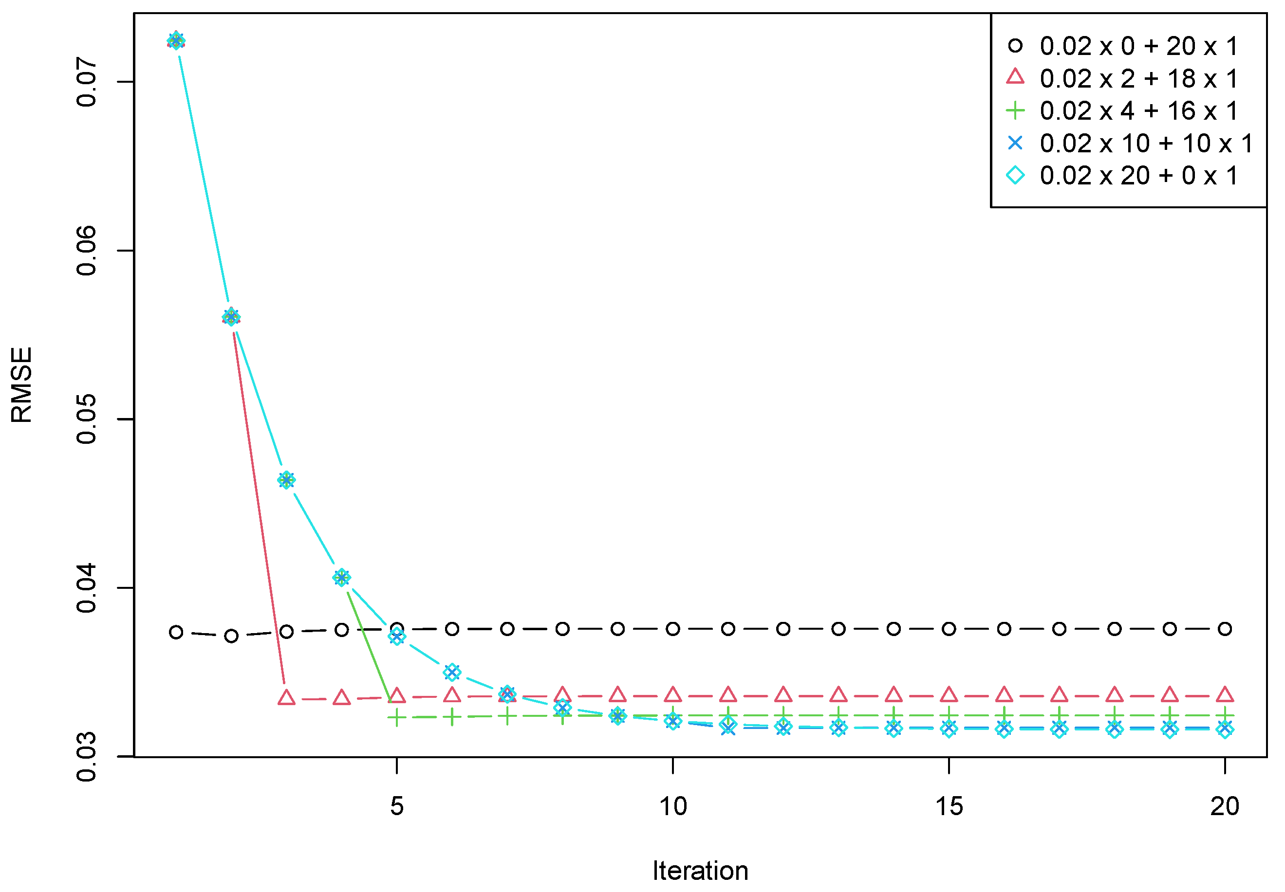
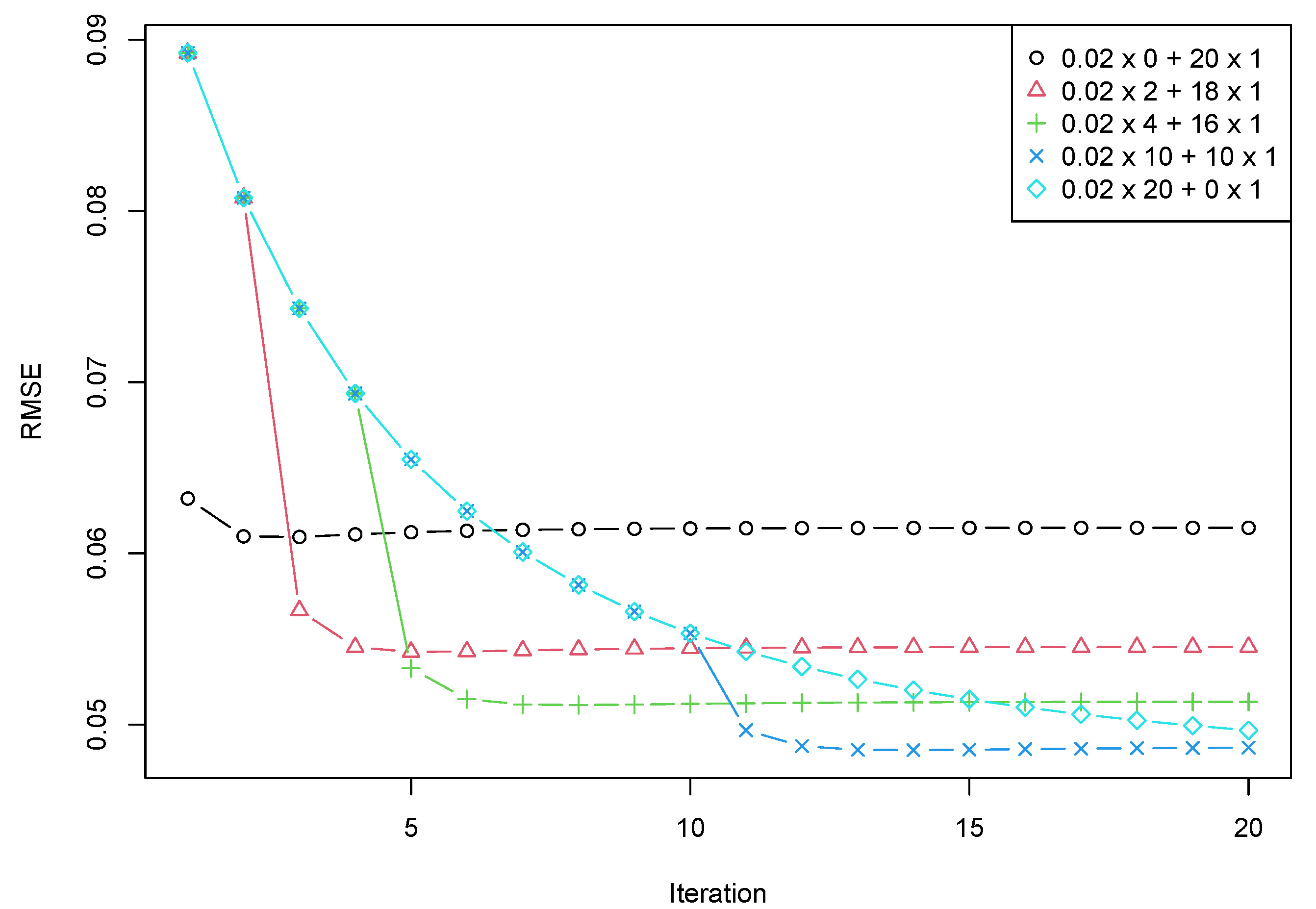
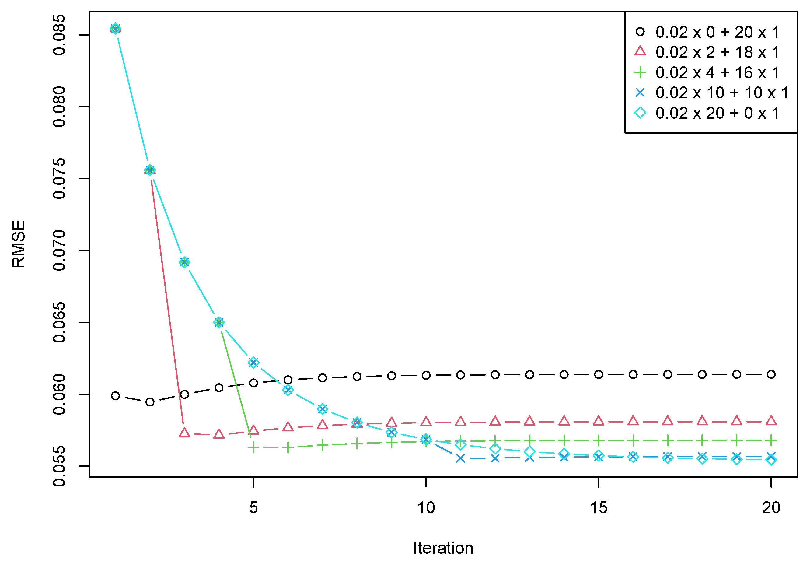
Main results. The main result consists of two parts. Theorem 2 contains the limit properties of (6) in the general case of alternating projections. Theorem 6, which is its corollary, is used to justify the proposed algorithm with mixed alternating projections for solving the problem (3). Section 5.2 demonstrates the capabilities of the proposed algorithm.

Paper’s structure. In this paper, we study general properties of alternating projections (Section 2) and mixed alternating projections (Section 3) and then apply them to Cadzow iterations with a justification of the choice of weights for the projectors participating in the mixed iterations. To do this, we consider a linearized version of the algorithm, where the projection on the set of rank-deficient matrices is replaced by the projection on the tangent subspace to the set of such matrices (Section 4). This allows us to apply the linear operator theory to the mixed iterations (Section 5). Section 5.1 discusses how the algorithm’s parameters affect the accuracy and rate of convergence. In Section 5.2, the obtained results are confirmed by a numerical experiment. Section 6 and Section 7 conclude the paper.

2. Alternating Projections

Consider the linear case where we are looking for a solution to an optimization problem

$$\underset{S\in \mathcal{A}\cap \mathcal{B}}{min}\parallel X-S\parallel ,$$

(7)

where $\mathcal{A}$ and $\mathcal{B}$ are linear subspaces of ${\mathbb{R}}^M$ with a nonempty intersection of dimension $m<M$.

The solution to the problem can be found using the method of alternating projections with an initial value of $S^{\left(0\right)}=X$ and the iteration step

$$S^{(k+1)}={\Pi }_{\mathcal{A}}{\Pi }_{\mathcal{B}}{S}^{\left(k\right)}.$$

(8)

The following statement is known.

Theorem 1

([15], Theorem 13.7).

$${\left({\Pi }_{\mathcal{A}}{\Pi }_{\mathcal{B}}\right)}^n\underset{n\to +\infty }{\to }{\Pi }_{\mathcal{A}\cap \mathcal{B}},$$

that is, the limit of the iterations is equal to the projection on the intersection of the subspaces $\mathcal{A}$ and $\mathcal{B}$.

This allows us to prove the following property. Denote ${\mathbf{P}}_{\mathcal{A},\mathcal{B}}={\Pi }_{\mathcal{A}}{\Pi }_{\mathcal{B}}$.

Corollary 1.

All the eigenvalues of the matrix ${\mathbf{P}}_{\mathcal{A},\mathcal{B}}$ lie within the unit circle; the eigenvalue $\lambda =1$, which only has modulus 1, is semi-simple and has multiplicity equal to $m=dim\mathcal{A}\cap \mathcal{B}$; the corresponding eigenvectors form the basis of $\mathcal{A}\cap \mathcal{B}$.

Proof. 

The statement of the corollary is obviously true in the case of diagonalizable matrix ${\mathbf{P}}_{\mathcal{A},\mathcal{B}}$, since by Theorem 1, ${\mathbf{P}}_{\mathcal{A},\mathcal{B}}^n$ tends to a projection matrix of rank m whose eigenvalues (1 of multiplicity m and 0 of multiplicity $M-m$) are the limits of the powers of the eigenvalues of ${\mathbf{P}}_{\mathcal{A},\mathcal{B}}$. In the general case, the result is based on the statement “Limits of Powers” in ([16], page 630), which, among other things, states that the eigenvalue 1 is semi-simple—i.e., its algebraic and geometric multiplicities coincide. The geometric multiplicity m of the unit root follows from the fact that the vectors from $\mathcal{A}\cap \mathcal{B}$ (and only they) correspond to the eigenvalue 1 of the matrix ${\mathbf{P}}_{\mathcal{A},\mathcal{B}}$. □

The following proposition establishes the convergence rate of alternating projections.

Proposition 1.

The following inequality holds:

$$\parallel ({\mathbf{P}}_{\mathcal{A},\mathcal{B}}^n-{\Pi }_{\mathcal{A}\cap \mathcal{B}})X\parallel \le C\parallel X\parallel \left(\right|\widehat{\lambda }{|+\delta )}^n,$$

(9)

where $C>0$ is some positive constant, $\delta >0$ is an arbitrarily small real number and $\widehat{\lambda }$ is the largest non-unit (that is, $(m+1)$-th) eigenvalue of the matrix ${\mathbf{P}}_{\mathcal{A},\mathcal{B}}$.

Proof. 

The theorem ([17], Theorem 2.12) implies that for a matrix $\mathbf{D}$, the convergence rate of ${\mathbf{D}}^k$ to the limit matrix ${\mathbf{D}}^{\infty }$ is determined by the spectral radius $\gamma =\rho (\mathbf{D}-{\mathbf{D}}^{\infty })$ of the difference matrix. Namely, for any $\mu >\gamma$, there exists a constant C such that $\parallel {\mathbf{D}}^k-{\mathbf{D}}^{\infty }\parallel \le C{\mu }^k$, where $\parallel ·\parallel$ is the induced norm. By Corollary 1, both matrices ${\mathbf{P}}_{\mathcal{A},\mathcal{B}}$ and ${\Pi }_{\mathcal{A}\cap \mathcal{B}}$ have eigenvalue one corresponding to the same eigenspace. Since the other eigenvalues of ${\Pi }_{\mathcal{A}\cap \mathcal{B}}$ are zero, the spectral radius of the difference matrix is $\widehat{\lambda }$, which proves the statement. □

Thus, the convergence rate of the algorithm with iterations given by (8) is determined by the modulus of the eigenvalue $|\widehat{\lambda }|$: the closer it is to one, the slower the algorithm converges.

Remark 1.

Using the commutativity property ${\Pi }_{\mathcal{A}\cap \mathcal{B}}{\Pi }_{\mathcal{A}}={\Pi }_{\mathcal{A}}{\Pi }_{\mathcal{A}\cap \mathcal{B}}={\Pi }_{\mathcal{A}\cap \mathcal{B}}$ and ${\Pi }_{\mathcal{A}\cap \mathcal{B}}{\Pi }_{\mathcal{B}}={\Pi }_{\mathcal{B}}{\Pi }_{\mathcal{A}\cap \mathcal{B}}={\Pi }_{\mathcal{A}\cap \mathcal{B}}$, the expression ${\mathbf{P}}_{\mathcal{A},\mathcal{B}}^n-{\Pi }_{\mathcal{A}\cap \mathcal{B}}$ on the left side of the inequality (9) can be rewritten as

$${\mathbf{P}}_{\mathcal{A},\mathcal{B}}^n-{\Pi }_{\mathcal{A}\cap \mathcal{B}}={\mathbf{P}}_{\widehat{\mathcal{A}},\widehat{\mathcal{B}}}^n,$$

where ${\mathbf{P}}_{\widehat{\mathcal{A}},\widehat{\mathcal{B}}}={\Pi }_{\widehat{\mathcal{A}}}{\Pi }_{\widehat{\mathcal{B}}}$, ${\Pi }_{\widehat{\mathcal{A}}}={\Pi }_{\mathcal{A}}-{\Pi }_{\mathcal{A}\cap \mathcal{B}}$, ${\Pi }_{\widehat{\mathcal{B}}}={\Pi }_{\mathcal{B}}-{\Pi }_{\mathcal{A}\cap \mathcal{B}}$, $\widehat{\mathcal{A}}$ and $\widehat{\mathcal{B}}$ are orthogonal complements of the $\mathcal{A}\cap \mathcal{B}$ in the subspaces $\mathcal{A}$ and $\mathcal{B}$, respectively. Then $\widehat{\lambda }$ is the largest absolute eigenvalue of the matrix ${\mathbf{P}}_{\widehat{\mathcal{A}},\widehat{\mathcal{B}}}$.

Let us show the relation of ${\mathbf{P}}_{\mathcal{A},\mathcal{B}}$ to canonical correlations and principal angles between subspaces.

Proposition 2.

Let $\mathbf{A}$ be the matrix consisting of a basis of the subspace $\mathcal{A}$ as its columns and $\mathbf{B}$ be the matrix consisting of a basis of the subspace $\mathcal{B}$ as its columns. Then, the following is true:

$${\mathbf{P}}_{\mathcal{A},\mathcal{B}}={\left({\mathbf{B}}^{\mathrm{T}}\mathbf{B}\right)}^{-1}\left({\mathbf{B}}^{\mathrm{T}}\mathbf{A}\right){\left({\mathbf{A}}^{\mathrm{T}}\mathbf{A}\right)}^{-1}\left({\mathbf{A}}^{\mathrm{T}}\mathbf{B}\right).$$

(10)

Proof. 

The formula (10) is obtained by multiplying the solutions of two least-squares approximation problems related to the subspaces $\mathcal{A}$ and $\mathcal{B}$. □

Remark 2.

The matrix on the right side of the equality (10) arises in the problem of computing canonical correlations. The squares of canonical correlations are equal to the squares of cosines of the so-called principal angles between subspaces $\mathcal{A}$ and $\mathcal{B}$, spanned by the columns of the matrices, and are calculated using the eigenvalues of this matrix.

Since we need only the leading principal angle, which is the angle between subspaces, we will use the simpler definition of the cosine of the angle between subspaces through the inner product.

Definition 1

([18]). Let $\mathcal{A}$ and $\mathcal{B}$ be two linear subspaces of a Hilbert space with inner product $\langle ·,·\rangle$ and the corresponding (semi-)norm $\parallel ·\parallel$. Then, the cosine of the angle between $\mathcal{A}$ and $\mathcal{B}$ is defined as

$$cos(\mathcal{A},\mathcal{B})=\underset{A\in \mathcal{A},B\in \mathcal{B}}{max}\left(\frac{|\langle A,B\rangle |}{\parallel A\parallel \parallel B\parallel }\right).$$

3. Mixed Alternating Projections

Suppose that different norms may be considered in the problem (7). For example, such a case arises if a weighted least-squares (WLS) problem is solved. Such a problem can be solved both with an optimal weight matrix in terms of the minimum error of WLS estimates and with some suboptimal ones.

Thus, consider two equivalent norms and assume that the application of the method of alternating projections in the first norm leads to a more accurate estimation of the solution, but the algorithm converges slowly, and alternating projections in the second norm, on the contrary, converge faster, but the accuracy of the solution is worse.

We propose a way to speed up the convergence of the algorithm using the first norm, almost without worsening the accuracy of the solution. Let us consider the projectors by two equivalent norms and denote the corresponding matrices ${\mathbf{P}}_{\mathcal{A},\mathcal{B}\left(1\right)}$ and ${\mathbf{P}}_{\mathcal{A},\mathcal{B}\left(2\right)}$. This notation is introduced and implies both projections in one of the 1st or 2nd norms in the definition ${\mathbf{P}}_{\mathcal{A},\mathcal{B}\left(i\right)}={\Pi }_{\mathcal{A}\left(i\right)}{\Pi }_{\mathcal{B}\left(i\right)}$, $i=1,2$.

The mixed alternating projections are defined as:

$$X_T={\mathbf{P}}_{\mathcal{A},\mathcal{B}\left(2\right)}^{T_2}{\mathbf{P}}_{\mathcal{A},\mathcal{B}\left(1\right)}^{T_1}{X}_0,$$

(11)

where $T=T_1+T_2$. Since this formula uses only linear operators, we can prove the main theorem of this paper.

Theorem 2.

For the algorithm given by (11), the following relations are true, where convergence is in the operator norm:

1. 

${\mathbf{P}}_{\mathcal{A},\mathcal{B}\left(2\right)}^{T_2}{\mathbf{P}}_{\mathcal{A},\mathcal{B}\left(1\right)}^{T_1}\to {\Pi }_{\mathcal{A}\cap \mathcal{B}\left(1\right)}$ if $T_2$ is fixed and $T_1\to +\infty$.

2. 

There exists an equivalent third norm such that ${\mathbf{P}}_{\mathcal{A},\mathcal{B}\left(2\right)}^{T_2}{\mathbf{P}}_{\mathcal{A},\mathcal{B}\left(1\right)}^{T_1}\to {\Pi }_{\mathcal{A}\cap \mathcal{B}\left(3\right)}$ if $T_1$ is fixed and $T_2\to +\infty$.

Proof. 

The proof of the first statement follows from Theorem 1: ${\mathbf{P}}_{\mathcal{A},\mathcal{B}\left(1\right)}^{T_1}\to {\Pi }_{\mathcal{A}\cap \mathcal{B}\left(1\right)}$ as $T_1\to +\infty$ and also ${\mathbf{P}}_{\mathcal{A},\mathcal{B}\left(2\right)}^{T_2}{\Pi }_{\mathcal{A}\cap \mathcal{B}\left(1\right)}={\Pi }_{\mathcal{A}\cap \mathcal{B}\left(1\right)}$ for any $T_2$.

To prove the second statement, we first apply Theorem 1 to the matrix ${\mathbf{P}}_{\mathcal{A},\mathcal{B}\left(2\right)}^{T_2}$ as $T_2\to +\infty$, and then consider the matrix $\tilde{\mathbf{P}}={\Pi }_{\mathcal{A}\cap \mathcal{B}\left(2\right)}{\mathbf{P}}_{\mathcal{A},\mathcal{B}\left(1\right)}^{T_1}$. It is sufficient to show that the matrix $\tilde{\mathbf{P}}$ defines a projection—i.e., $\tilde{\mathbf{P}}=\tilde{\mathbf{P}}\tilde{\mathbf{P}}$; then, the required projection is $\tilde{\mathbf{P}}={\Pi }_{\mathcal{A}\cap \mathcal{B}\left(3\right)}$ in a third norm. By using direct substitution, we obtain:

$$\tilde{\mathbf{P}}\tilde{\mathbf{P}}={\Pi }_{\mathcal{A}\cap \mathcal{B}\left(2\right)}\left({\mathbf{P}}_{\mathcal{A},\mathcal{B}\left(1\right)}^{T_1}{\Pi }_{\mathcal{A}\cap \mathcal{B}\left(2\right)}\right){\mathbf{P}}_{\mathcal{A},\mathcal{B}\left(1\right)}^{T_1}.$$

Since ${\mathbf{P}}_{\mathcal{A},\mathcal{B}\left(1\right)}^{T_1}{\Pi }_{\mathcal{A}\cap \mathcal{B}\left(2\right)}={\Pi }_{\mathcal{A}\cap \mathcal{B}\left(2\right)}$ for any $T_1$, the second statement is proved. □

Theorem 2 has the following interpretation: if one first makes $T_1$ steps with projections in the first norm in the iteration (11), and then iterates with projections in the second norm, then the obtained result will still be a projection on the desired subspace (item 2), and the larger $T_1$ is, the closer this projection will be to the projection in the first norm (item 1). This implies that to achieve fast and accurate estimation, the first norm should correspond to a more accurate solution of the problem and possibly slower convergence of the alternating projections, and the second norm can correspond to a less accurate solution but faster iterations. The rate of convergence of the corresponding operators is explained by Proposition 1.

A general rule in optimization is that the accuracy of two successive optimization methods is inherited from the second method, so the first method is chosen to be fast and possibly inaccurate, and the second method to be more accurate. Theorem 2 shows that in alternating projections, the situation is in some sense the opposite. This can be explained as follows. Optimization methods use the target function at each step, and can therefore adjust the steps. In the case of alternating projections, initial data are used only to compute the first iteration. Therefore, it is important to perform the first iterations in the proper direction.

4. Linearized Cadzow Iterations in the Signal-Estimation Problem

In the next Section 5, we apply the approach proposed in Section 3 to solving the SLRA problem (3) to estimate signals in time series. Since this approach considers alternating projections to linear subspaces, we start with linearization of the Cadzow iteration (5). The Cadzow iteration is not linear because it uses the projection onto the nonconvex set ${\mathcal{M}}_r$ of matrices of rank not larger than r, which is not a closed subspace but is a smooth manifold [19].

Let us sketch the way of linearization in the neighborhood of a time series ${\mathsf{S}}_0\in {\mathcal{D}}_r$ of rank r. First, we consider the set ${\mathcal{M}}_r$ in the neighborhood of the point ${\mathbf{S}}_0={\mathcal{T}}_L\left({\mathsf{S}}_0\right)$. The projection in the neighborhood of this point is correctly defined if we solve the signal-estimation problem for a noisy time series of the form $\mathsf{X}={\mathsf{S}}_0+\xi$, where $\xi$ is a random vector with a zero mean and an autocovariance matrix proportional to ${\mathbf{W}}_0^{-1}={\Sigma }_0$, where the variances are small enough and ${\mathbf{W}}_0$ is a given weight matrix. After that, we construct a linearized iteration by replacing the set ${\mathcal{M}}_r$ with a tangent subspace at ${\mathbf{S}}_0$. Then, we can reduce the linearized iteration to a multiplication by a real matrix and find its properties. As a result, we obtain asymptotic relations for the linearization which explains the yield of the full Cadzow iteration (5).

4.1. Linearization of the Operator ${\Pi }_{{\mathcal{M}}_r,(\mathbf{L},\mathbf{R})}$

Consider the matrix ${\mathbf{S}}_0\in {\mathbb{R}}^{L\times K}$, $L>r$ and $K>r$, where ${\mathbf{S}}_0={\mathcal{T}}_L\left({\mathsf{S}}_0\right)$ and ${\mathsf{S}}_0$ is a series of rank r; hence, the matrix ${\mathbf{S}}_0$ has rank r. In the neighborhood of the point ${\mathbf{S}}_0$, the set ${\mathcal{M}}_r$ is a smooth manifold of dimension $r(L+K)-r^2$, and the tangent subspace $\mathcal{N}=\mathcal{N}\left({\mathbf{S}}_0\right)$ at ${\mathbf{S}}_0$ is expressed as follows [19]:

$$\mathcal{N}\left({\mathbf{S}}_0\right)=\{\mathbf{X}\in {\mathbb{R}}^{L\times K}:{\mathbf{U}}^{\mathrm{T}}\mathbf{X}\mathbf{V}={\mathbf{0}}_{L-r,K-r}\},$$

(12)

where $\mathbf{U}\in {\mathbb{R}}^{L\times (L-r)}$ and $\mathbf{V}\in {\mathbb{R}}^{K\times (K-r)}$ are arbitrary full-rank matrices such that ${\mathbf{U}}^{\mathrm{T}}{\mathbf{S}}_0={\mathbf{0}}_{L-r,K}$ and ${\mathbf{S}}_0\mathbf{V}={\mathbf{0}}_{L,K-r}$. Note that the definition is correct because $\mathcal{N}\left({\mathbf{S}}_0\right)$ depends only on $\mathrm{colspace}{\mathbf{S}}_0$ and $\mathrm{rowspace}{\mathbf{S}}_0$.

Let us denote by ${\Pi }_{\mathcal{N}\left({\mathbf{S}}_0\right),(\mathbf{L},\mathbf{R})}:{\mathbb{R}}^{L\times K}\to \mathcal{N}\left({\mathbf{S}}_0\right)$ the projection on $\mathcal{N}\left({\mathbf{S}}_0\right)$ in the norm generated by (4). Then, the linearized Cadzow iteration in the neighborhood of the point ${\mathbf{S}}_0$ has the following form:

$${\mathbf{X}}_{k+1}={\Pi }_{\mathcal{H},(\mathbf{L},\mathbf{R})}{\Pi }_{\mathcal{N}\left({\mathbf{S}}_0\right),(\mathbf{L},\mathbf{R})}{\mathbf{X}}_k.$$

(13)

Set ${\mathbf{X}}_0={\mathcal{T}}_L\left({\mathsf{X}}_0\right)$, ${\mathsf{X}}_k={\mathcal{T}}_L^{-1}\left({\mathbf{X}}_k\right)$, $k\ge 1$. Then, we can rewrite (13) as

$${\mathsf{X}}_{k+1}=\left({\mathcal{T}}_L^{-1}{\Pi }_{\mathcal{H},(\mathbf{L},\mathbf{R})}{\Pi }_{\mathcal{N}\left({\mathbf{S}}_0\right),(\mathbf{L},\mathbf{R})}{\mathcal{T}}_L\right){\mathsf{X}}_k.$$

Note that each of the operators inside the brackets is linear. Hence, their composition is a linear operator and therefore can be written as a matrix, which we denote ${\mathbf{P}}_{{\mathsf{S}}_0,(\mathbf{L},\mathbf{R})}$:

$${\mathbf{P}}_{{\mathsf{S}}_0,(\mathbf{L},\mathbf{R})}={\mathcal{T}}_L^{-1}{\Pi }_{\mathcal{H},(\mathbf{L},\mathbf{R})}{\Pi }_{\mathcal{N}\left({\mathbf{S}}_0\right),(\mathbf{L},\mathbf{R})}{\mathcal{T}}_L,{\mathsf{X}}_{k+1}={\mathbf{P}}_{{\mathsf{S}}_0,(\mathbf{L},\mathbf{R})}{\mathsf{X}}_k.$$

(14)

Formally, we can calculate the elements of the matrix ${\mathbf{P}}_{{\mathsf{S}}_0,(\mathbf{L},\mathbf{R})}$ by successive substituting N standard unit vectors into the composition of operators.

4.2. Intersection of Subspaces $\mathcal{H}\cap \mathcal{N}\left({\mathbf{S}}_0\right)$

For a compact representation of the further results, let us describe the intersection of the tangent subspace to the set of matrices of finite rank ${\mathcal{M}}_r$ and the space of Hankel matrices $\mathcal{H}$.

Let us gather necessary definitions from [12].

Definition 2.

We say that a series ${\mathsf{S}}_0\in {\mathbb{R}}^N$ is governed by a generalized linear recurrence relation (GLRR) with coefficients $\mathbf{a}$, where $\mathbf{a}\in {\mathbb{R}}^{r+1}$ and $\mathbf{a}\ne {\mathbf{0}}_{r+1}$, if ${\mathbf{a}}^{\mathrm{T}}{\mathcal{T}}_{r+1}\left({\mathsf{S}}_0\right)={\mathbf{0}}_{N-r}^{\mathrm{T}}$. We denote by ${\mathcal{Z}}_N\left(\mathbf{a}\right)=\mathcal{Z}\left(\mathbf{a}\right)=\{\mathsf{S}\in {\mathbb{R}}^N:{\mathbf{a}}^{\mathrm{T}}{\mathcal{T}}_{r+1}\left(\mathsf{S}\right)={\mathbf{0}}_{N-r}^{\mathrm{T}}\}$ the subspace of time series governed by the GLRR($\mathbf{a}$).

Consider an equivalent form of $\mathcal{Z}\left(\mathbf{a}\right)$. Denote by ${\mathbf{Q}}^{M,d}$ the operator ${\mathbb{R}}^{d+1}\to {\mathbb{R}}^{M\times (M-d)}$ defined as follows:

$${\mathbf{Q}}^{M,d}\left(\mathbf{b}\right)=\left(\begin{array}{cccc}{b}_1& 0& \cdots & 0\\ b_2& b_1& 0& ⋮\\ ⋮& b_2& \ddots & 0\\ b_{d+1}& ⋮& \ddots & b_1\\ 0& b_{d+1}& \ddots & b_2\\ ⋮& 0& \ddots & ⋮\\ 0& \cdots & 0& b_{d+1}\end{array}\right),$$

(15)

where $\mathbf{b}={(b_1,\dots ,b_{d+1})}^{\mathrm{T}}\in {\mathbb{R}}^{d+1}$. Then, $\mathcal{Z}\left(\mathbf{a}\right)$ can be represented in another form as

$$\mathcal{Z}\left(\mathbf{a}\right)=\{\mathsf{S}\in {\mathbb{R}}^N:{\mathbf{Q}}^{\mathrm{T}}\left(\mathbf{a}\right)\mathsf{S}=0_{N-r}\},$$

(16)

where $\mathbf{Q}={\mathbf{Q}}^{N,r}$ [20].

Remark 3.

Since the columns and rows of the trajectory matrix of a time series in ${\mathcal{D}}_r$ satisfy the same GLRR($\mathbf{a}$) as the original series does, we can take ${\mathbf{Q}}^{L,r}\left(\mathbf{a}\right)$ and ${\mathbf{Q}}^{K,r}\left(\mathbf{a}\right)$ as $\mathbf{U}$ and $\mathbf{V}$ in (12), respectively.

Definition 3.

Let $\mathbf{a}={(a_1,\dots ,a_k)}^{\mathrm{T}}\in {\mathbb{R}}^k$. Denote by ${\mathbf{a}}^2\in {\mathbb{R}}^{2k-1}={(a_1^{\left(2\right)},\dots ,a_{2k-1}^{\left(2\right)})}^{\mathrm{T}}$ the acyclic convolution of the vector with itself:

$$a_i^{\left(2\right)}=\sum _{j=max(1,i-k+1)}^{min(i,k)}{a}_j{a}_{i-j+1}.$$

(17)

As shown in [12], the tangent subspace to ${\mathcal{D}}_r$ at ${\mathsf{S}}_0$ coincides with $\mathcal{Z}\left({\mathbf{a}}_0^2\right)$, $dim\mathcal{Z}\left({\mathbf{a}}_0^2\right)=2r$. The following theorem establishes the relation between the tangent subspaces to the manifold of time series governed by GLRRs and the manifold of their trajectory matrices.

Theorem 3.

Let ${\mathsf{S}}_0\in {\mathcal{D}}_r$; i.e., let ${\mathsf{S}}_0$ be a series of rank r, $r<min(L,K)$, and ${\mathsf{S}}_0\in \mathcal{Z}\left({\mathbf{a}}_0\right)$—i.e., let ${\mathsf{S}}_0$ be governed by the GLRR(${\mathbf{a}}_0$) for a vector ${\mathbf{a}}_0\in {\mathbb{R}}^{r+1}$. Then, ${\mathcal{T}}_L^{-1}(\mathcal{H}\cap \mathcal{N}\left({\mathbf{S}}_0\right))=\mathcal{Z}\left({\mathbf{a}}_0^2\right)$, where ${\mathbf{S}}_0={\mathcal{T}}_L\left({\mathsf{S}}_0\right)$.

Proof. 

Consider a matrix $\mathbf{X}$ in the intersection of $\mathcal{H}$ and $\mathcal{N}\left({\mathbf{S}}_0\right)$. In particular, there exists $\mathsf{X}={(x_1,\dots ,x_N)}^{\mathrm{T}}$: $\mathbf{X}={\mathcal{T}}_L\left(\mathsf{X}\right)$. Let us calculate the $(i,j)$-th element of the matrix ${\mathbf{U}}^{\mathrm{T}}\mathbf{X}\mathbf{V}$ from (12) following Remark 3:

$$\sum _{l=1}^{r+1}\sum _{p=1}^{r+1}{a}_l{a}_p{x}_{i+l-1+p+j-1-1}=\sum _{l=1}^{r+1}\sum _{p=1}^{r+1}{a}_l{a}_p{x}_{(i+j-1)+p+l-2}=\sum _{k=1}^{2r+1}{a}_k^{\left(2\right)}{x}_{(i+j-1)+k-1}=0,$$

(18)

where $a_i^{\left(2\right)}$ are coefficients of the vector ${\mathbf{a}}_0^2$; see definition (17). The values of $i+j-1$, where i runs from 1 to $L-r$ and j runs from 1 to $K-r$, cover the entire interval from 1 to $N-2r$, and therefore, (18) is equivalent to ${\left(\mathbf{Q}\left({\mathbf{a}}^2\right)\right)}^{\mathrm{T}}\mathsf{X}={\mathbf{0}}_{N-2r}$. Thus, according to (16), all such $\mathsf{X}$ constitute $\mathcal{Z}\left({\mathbf{a}}^2\right)$. □

4.3. Limit Property of the Composition of Projections

First, consider the relation connecting the (semi-)norm ${\parallel \mathsf{Z}\parallel }_{\mathbf{W}}$ generated by the inner product (2) and the (semi-)norm ${\parallel \mathbf{Z}\parallel }_{\mathbf{L},\mathbf{R}}$, which is generated by the inner product (4) (semi-norms arise if not to require nondegeneracy of the matrices $\mathbf{W}$, $\mathbf{L}$ and $\mathbf{R}$). The mapping ${\mathcal{T}}_L$ preserves the norm if ${\parallel \mathsf{Z}\parallel }_{\mathbf{W}}={\parallel \mathbf{Z}\parallel }_{\mathbf{L},\mathbf{R}}$ for any $\mathsf{Z}$, where $\mathbf{Z}={\mathcal{T}}_L\left(\mathsf{Z}\right)$, $\mathbf{L}$ and $\mathbf{R}$ are matrix weights and $\mathbf{W}$ is a weight matrix.

Define the convolution of the two matrices $\mathbf{C}=\mathbf{A}\ast \mathbf{B}$ for $\mathbf{A}\in {\mathbb{R}}^{L\times L}$, $\mathbf{B}\in {\mathbb{R}}^{K\times K}$ and $\mathbf{C}\in {\mathbb{R}}^{N\times N}$ as

$$c_{i,j}=\sum _{i_1+i_2-1=i}\sum _{j_1+j_2-1=j}{a}_{i_1,j_1}{b}_{i_2{j}_2},$$

where $\mathbf{A}=\left(a_{i_1,j_1}\right)$, $\mathbf{B}=\left(b_{i_2,j_2}\right)$ and $\mathbf{C}=\left(c_{i,j}\right)$.

There is a known relation linking the weight matrix to the matrix weights.

Theorem 4

([8]). ${\parallel \mathsf{Z}\parallel }_{\mathbf{W}}={\parallel \mathbf{Z}\parallel }_{\mathbf{L},\mathbf{R}}$ for any series $\mathsf{Z}\in {\mathbb{R}}^N$ if and only if $\mathbf{W}=\mathbf{W}(\mathbf{L},\mathbf{R})=\mathbf{L}\ast \mathbf{R}$.

All statements of the following theorem are a direct application of Theorem 1 and Proposition 1 with consideration to

$${\mathbf{P}}_{{\mathsf{S}}_0,(\mathbf{L},\mathbf{R})}^n={\left({\mathcal{T}}_L^{-1}{\Pi }_{\mathcal{H},(\mathbf{L},\mathbf{R})}{\Pi }_{\mathcal{N}\left({\mathbf{S}}_0\right),(\mathbf{L},\mathbf{R})}{\mathcal{T}}_L\right)}^n={\mathcal{T}}_L^{-1}{\left({\Pi }_{\mathcal{H},(\mathbf{L},\mathbf{R})}{\Pi }_{\mathcal{N}\left({\mathbf{S}}_0\right),(\mathbf{L},\mathbf{R})}\right)}^n{\mathcal{T}}_L$$

and ${\mathcal{T}}_L^{-1}(\mathcal{H}\cap \mathcal{N}\left({\mathbf{S}}_0\right))=\mathcal{Z}\left({\mathbf{a}}_0^2\right)$.

Theorem 5.

Let ${\mathsf{S}}_0$ be a time series governed by a GLRR(${\mathbf{a}}_0$), ${\mathbf{S}}_0={\mathcal{T}}_L\left({\mathsf{S}}_0\right)$. Then

1. 

The following operator convergence takes place:

$${\left({\Pi }_{\mathcal{H},(\mathbf{L},\mathbf{R})}{\Pi }_{\mathcal{N}\left({\mathbf{S}}_0\right),(\mathbf{L},\mathbf{R})}\right)}^n\underset{n\to +\infty }{\to }{\Pi }_{\mathcal{H}\cap \mathcal{N}\left({\mathbf{S}}_0\right),(\mathbf{L},\mathbf{R})},$$

that is, the limit of iterations is equal to the projection on the intersection of the subspaces $\mathcal{H}$ and $\mathcal{N}\left({\mathbf{S}}_0\right)$.

2. 

The following matrix convergence is valid:

$${\mathbf{P}}_{{\mathsf{S}}_0,(\mathbf{L},\mathbf{R})}^n\underset{n\to +\infty }{\to }{\Pi }_{\mathcal{Z}\left({\mathbf{a}}_0^2\right),\mathbf{L}\ast \mathbf{R}},$$

where ${\Pi }_{\mathcal{X},\mathbf{W}}$ denotes the matrix of projection on the linear subspace $\mathcal{X}$ in the norm generated by the inner product (2) with the weight matrix $\mathbf{W}$.

3. 

All the eigenvalues of the matrix ${\mathbf{P}}_{{\mathsf{S}}_0,(\mathbf{L},\mathbf{R})}$ lie within the unit circle; the eigenvalue $\lambda =1$, which only has modulus 1, is semi-simple and has multiplicity equal to $2r$; the corresponding eigenvectors form the basis of $\mathcal{Z}\left({\mathbf{a}}_0^2\right)$. If the weight matrix $\mathbf{W}$ is nondegenerate,

$$\parallel ({\mathbf{P}}_{{\mathsf{S}}_0,(\mathbf{L},\mathbf{R})}^n-{\Pi }_{\mathcal{Z}\left({\mathbf{a}}_0^2\right),\mathbf{L}\ast \mathbf{R}}){\mathsf{X}\parallel }_{\mathbf{W}}\le {C\parallel \mathsf{X}\parallel }_{\mathbf{W}}\left(\right|\widehat{\lambda }{|+\delta )}^n,$$

(19)

where C is some positive constant, $\delta >0$ is any small real number, $\widehat{\lambda }$ is the largest non-unitary (that is, $(2r+1)$-th) eigenvalue of the matrix ${\mathbf{P}}_{{\mathsf{S}}_0,(\mathbf{L},\mathbf{R})}$.

4.4. Influences of the Matrices $\mathbf{L}$ and $\mathbf{R}$ on the First Principal Angle and Convergence Rate of the Cadzow Method

Recall that if one wants to solve the problem (1) for a given weight matrix $\mathbf{W}$ using the Cadzow method, one must require $\mathbf{W}=\mathbf{L}\ast \mathbf{R}$. To obtain the maximum likelihood estimate, the matrix $\mathbf{W}$ is chosen as the inverse of the noise autocovariance matrix. However, for such weight matrices $\mathbf{W}$ in the case of white or autoregressive noise, there are no nondegenerate matrix weights $\mathbf{L}$ and $\mathbf{R}$. Therefore, the matrix weights $\mathbf{L}$ and $\mathbf{R}$ are sought numerically under the upper bound $1/\alpha$ of the condition number of $\mathbf{R}$ for a given $\mathbf{L}$.

The works [13,14] are devoted to the search for appropriate matrix weights. To find these weights, the matrix $\mathbf{L}$ was fixed in some specific way, and the diagonal matrix $\mathbf{R}$ was numerically found such that the measure of discrepancy considered in these papers was minimal: $\rho (\mathbf{W},\mathbf{L}\ast \mathbf{R})\to {min}_{\mathbf{R}}$ provided $\mathrm{cond}\mathbf{R}\le 1/\alpha$, where $0<\alpha \le 1$. Simulations have shown that the control of matrix conditionality by the parameter $\alpha$ affects the convergence rate of the Cadzow method and the estimation accuracy. Decreasing $\alpha$ increases the set on which the matrix $\mathbf{R}$ is matched; this allows us to obtain a weight matrix with smaller values of $\rho (\mathbf{W},\mathbf{L}\ast \mathbf{R})$ and leads to improved accuracy of the signal estimate. However, decreasing $\alpha$ also results in slower convergence of the iterations, which requires a theoretical explanation. A general theoretical dependence on $\alpha$ could not be obtained, so we demonstrate the convergence rate when $\alpha$ tends to zero.

We know from Theorem 5 that the convergence rate of the methods is affected by the $(2r+1)$-th eigenvalues of the matrix ${\mathbf{P}}_{{\mathsf{S}}_0,(\mathbf{L},\mathbf{R})}$. From Remark 2, we know that this eigenvalue is equal to the squared cosine of the $(2r+1)$-th angle between the corresponding subspaces.

The calculation of the cosine of the $(2r+1)$-th principal angle between $\mathcal{H}$ and $\mathcal{N}\left({\mathbf{S}}_0\right)$ can be reduced to finding the cosine between the orthogonal (in the inner product ${\langle ·,·\rangle }_{\mathbf{L},\mathbf{R}}$, given in (4)) complements to $\mathcal{H}\cap \mathcal{N}\left({\mathbf{S}}_0\right)$ in $\mathcal{H}$ and $\mathcal{N}\left({\mathbf{S}}_0\right)$, respectively. Let us denote these complements $\widehat{\mathcal{H}}(\mathbf{L},\mathbf{R})$ and $\widehat{\mathcal{N}}({\mathbf{S}}_0,\mathbf{L},\mathbf{R})$. Note that by Theorem 3, $\mathcal{H}\cap \mathcal{N}\left({\mathbf{S}}_0\right)={\mathcal{T}}_L\left(\mathcal{Z}\left({\mathbf{a}}_0^2\right)\right)$, and its rank equals $2r$. For brevity, we will omit ${\mathbf{S}}_0$ in $\widehat{\mathcal{N}}({\mathbf{S}}_0,\mathbf{L},\mathbf{R})$ and $\mathcal{N}\left({\mathbf{S}}_0\right)$.

The properties of the principal angles concerning Remark 1 lead directly to the following statement.

Proposition 3.

The cosine of the $(2r+1)$-th principal angle between the subspaces $\mathcal{H}$ and $\mathcal{N}$ is equal to $cos(\widehat{\mathcal{H}}(\mathbf{L},\mathbf{R}),\widehat{\mathcal{N}}(\mathbf{L},\mathbf{R}))$.

4.4.1. Example of Bad Convergence as $\alpha$ Tends to Zero

Using Proposition 3 and the fact that the cosine of the $(2r+1)$-th principal angle determines the convergence rate (Proposition 1), we show by a specific example that this cosine tends to one as $\alpha$ tends to zero; this makes the convergence of the linearized Cadzow algorithm as slow as possible.

Let $N=2L$ and $K=L+1$. Let the matrix weights $\mathbf{L}={\mathbf{I}}_L$ be the identity matrix, which corresponds to the case of white noise. For simplicity, we make the matrix $\mathbf{R}=\mathbf{R}\left(\alpha \right)\in {\mathbb{R}}^{K\times K}$ equal to $\mathbf{R}=\mathrm{diag}(1,\alpha ,\dots ,\alpha ,1)$ according to [13]. Numerical experiments show that similar matrix weights (up to multiplying a constant) are obtained when applying the method from [12] of finding weights for small $\alpha$. Consider the degenerate case $\mathbf{R}\left(0\right)$ studied in [13].

Proposition 4.

For any matrix $\mathbf{X}\in {\mathbb{R}}^{L\times (L+1)}$, we can find a matrix $\mathbf{Y}\in \mathcal{H}$ such that ${\parallel \mathbf{X}-\mathbf{Y}\parallel }_{{\mathbf{I}}_L,\mathbf{R}\left(0\right)}=0$.

Proof. 

The inner product (4) of matrices ${\mathbf{Z}}_1$ and ${\mathbf{Z}}_2$ with the matrix weights $\mathbf{L}={\mathbf{I}}_L$ and $\mathbf{R}\left(0\right)=\mathrm{diag}(1,0,\dots ,0,1)$ depends only on the first and last columns of these matrices due to the form of $\mathbf{R}\left(0\right)$. Therefore, the required matrix $\mathbf{Y}$ can be written in the form $\mathbf{Y}={\Pi }_{\mathcal{H},({\mathbf{I}}_L,\mathbf{R}\left(0\right))}\mathbf{X}$, where the projection is calculated uniquely using the values from the first and last columns of the matrix $\mathbf{X}$. □

Corollary 2.

Let $\mathbf{X}\in {\mathbb{R}}^{L\times (L+1)}$ be an arbitrary matrix, $\widehat{\mathbf{X}}=\mathbf{X}-{\Pi }_{{\mathcal{T}}_L\left(\mathcal{Z}\left({\mathbf{a}}_0^2\right)\right),({\mathbf{I}}_L,\mathbf{R}\left(0\right))}\mathbf{X}$, $\widehat{\mathbf{Y}}={\Pi }_{\widehat{\mathcal{H}}({\mathbf{I}}_L,\mathbf{R}\left(0\right)),({\mathbf{I}}_L,\mathbf{R}\left(0\right))}\widehat{\mathbf{X}}$. Then, $\parallel \widehat{\mathbf{X}}-\widehat{\mathbf{Y}}{\parallel }_{{\mathbf{I}}_L,\mathbf{R}\left(0\right)}=0$.

Proof. 

The corollary is proved by the following substitution:

${\Pi }_{\widehat{\mathcal{H}}({\mathbf{I}}_L,\mathbf{R}\left(0\right)),({\mathbf{I}}_L,\mathbf{R}\left(0\right))}={\Pi }_{\mathcal{H},({\mathbf{I}}_L,\mathbf{R}\left(0\right))}-{\Pi }_{{\mathcal{T}}_L\left(\mathcal{Z}\left({\mathbf{a}}_0^2\right)\right),({\mathbf{I}}_L,\mathbf{R}\left(0\right))}$. □

Corollary 3.

Let $\mathbf{N}\in \mathcal{N}\left({\mathbf{S}}_0\right)$. Denote $\widehat{\mathbf{N}}\left(\alpha \right)={\Pi }_{\widehat{\mathcal{N}}({\mathbf{I}}_L,\mathbf{R}\left(\alpha \right)),({\mathbf{I}}_L,\mathbf{R}\left(\alpha \right))}\mathbf{N}$ and $\widehat{\mathbf{H}}\left(\alpha \right)={\Pi }_{\widehat{\mathcal{H}}({\mathbf{I}}_L,\mathbf{R}\left(\alpha \right)),({\mathbf{I}}_L,\mathbf{R}\left(\alpha \right))}\widehat{\mathbf{N}}\left(\alpha \right)$. Then, the following is fulfilled:

$$\begin{array}{c}\parallel \widehat{\mathbf{N}}{\left(\alpha \right)\parallel }_{{\mathbf{I}}_L,\mathbf{R}\left(\alpha \right)}\underset{\alpha \to 0}{\to }{\parallel \widehat{\mathbf{N}}\left(0\right)\parallel }_{{\mathbf{I}}_L,\mathbf{R}\left(0\right)},\\ \parallel \widehat{\mathbf{H}}{\left(\alpha \right)\parallel }_{{\mathbf{I}}_L,\mathbf{R}\left(\alpha \right)}\underset{\alpha \to 0}{\to }{\parallel \widehat{\mathbf{H}}\left(0\right)\parallel }_{{\mathbf{I}}_L,\mathbf{R}\left(0\right)},\\ \parallel \widehat{\mathbf{N}}{\left(0\right)\parallel }_{{\mathbf{I}}_L,\mathbf{R}\left(0\right)}={\parallel \widehat{\mathbf{H}}\left(0\right)\parallel }_{{\mathbf{I}}_L,\mathbf{R}\left(0\right)},\\ {\langle \widehat{\mathbf{N}}\left(\alpha \right),\widehat{\mathbf{H}}\left(\alpha \right)\rangle }_{{\mathbf{I}}_L,\mathbf{R}\left(\alpha \right)}\underset{\alpha \to 0}{\to }{\parallel \widehat{\mathbf{N}}\left(0\right)\parallel }_{{\mathbf{I}}_L,\mathbf{R}\left(0\right)}^2.\end{array}$$

Proof. 

Since $\widehat{\mathbf{N}}\left(\alpha \right)=\mathbf{N}-{\Pi }_{{\mathcal{T}}_L\left(\mathcal{Z}\left({\mathbf{a}}_0^2\right)\right),({\mathbf{I}}_L,\mathbf{R}\left(\alpha \right))}\mathbf{N}$, this expression is smooth in $\alpha$ and uniquely defined when $\alpha =0$. The projection ${\Pi }_{\widehat{\mathcal{H}}({\mathbf{I}}_L,\mathbf{R}\left(\alpha \right)),({\mathbf{I}}_L,\mathbf{R}\left(\alpha \right))}$ is also smooth in $\alpha$ and uniquely defined at $\alpha =0$. Applying Corollary 2 for $\mathbf{X}=\mathbf{N}$ and $\alpha =0$, we obtain that $\parallel \widehat{\mathbf{N}}\left(0\right)-\widehat{\mathbf{H}}{\left(0\right)\parallel }_{{\mathbf{I}}_L,\mathbf{R}\left(0\right)}=0$; this yields the statements of the corollary due to the smoothness of the left-side and right-side expressions. □

The declared result is described in the following proposition.

Proposition 5.

Let $L>2r>0$ and $N=2L$. Then,

$$cos(\widehat{\mathcal{H}}({\mathbf{I}}_L,\mathbf{R}\left(\alpha \right)),\widehat{\mathcal{N}}({\mathbf{I}}_L,\mathbf{R}\left(\alpha \right))\underset{\alpha \to 0}{\to }1.$$

Proof. 

Note that the cosine of the angle between a vector and a subspace (see Definition 1) is equal to the cosine between this vector and its projection to the subspace. Thus, we can use Corollary 3. It follows from Corollary 3 that the numerator and denominator in the definition of cosine are equal, and therefore, it is sufficient to prove that $\parallel \widehat{\mathbf{N}}{\left(0\right)\parallel }_{{\mathbf{I}}_L,\mathbf{R}\left(0\right)}\ne 0$. The latter can be shown by constructing such a matrix $\widehat{\mathbf{N}}\left(0\right)$ from the trajectory matrix ${\mathbf{S}}_0={\mathcal{T}}_L\left({\mathsf{S}}_0\right)$.

Let $S^{\mathrm{T}}$ be a row of the matrix ${\mathbf{S}}_0$ with a non-zero element at the first or last position (such a row always exists since ${\mathsf{S}}_0\ne 0$). Without loss of generality, we suppose that the first element of $S^{\mathrm{T}}$ is not zero. Denote $\mathcal{G}:{\mathbb{R}}^N\to {\mathbb{R}}^L$ the mapping that truncates the vector to the first L coordinates. Then, let $Q\in {\mathbb{R}}^L$ be a nonzero vector, which does not lie in $\mathcal{G}\left(\mathcal{Z}\left({\mathbf{a}}_0^2\right)\right)$, and $\mathbf{N}=Q{S}^{\mathrm{T}}$. By construction, $\mathbf{N}\in \mathcal{N}({\mathbf{S}}_0,\mathbf{L},\mathbf{R})$ and $\widehat{\mathbf{N}}\left(0\right)$ have a nonzero first column, and therefore, $\parallel \widehat{\mathbf{N}}{\left(0\right)\parallel }_{{\mathbf{I}}_L,\mathbf{R}\left(0\right)}\ne 0$. □

Thus, for a popular case $N=2L$, we have shown that the cosine of the $(2r+1)$-th principal angle can be as close to 1 as one wishes; hence, the convergence of the Cadzow method becomes as slow as one chooses with a small $\alpha$. Recall that the sense of choosing a small $\alpha$ is to increase the estimation accuracy.

4.4.2. Numerical Example for the Dependence of Convergence on $\alpha$

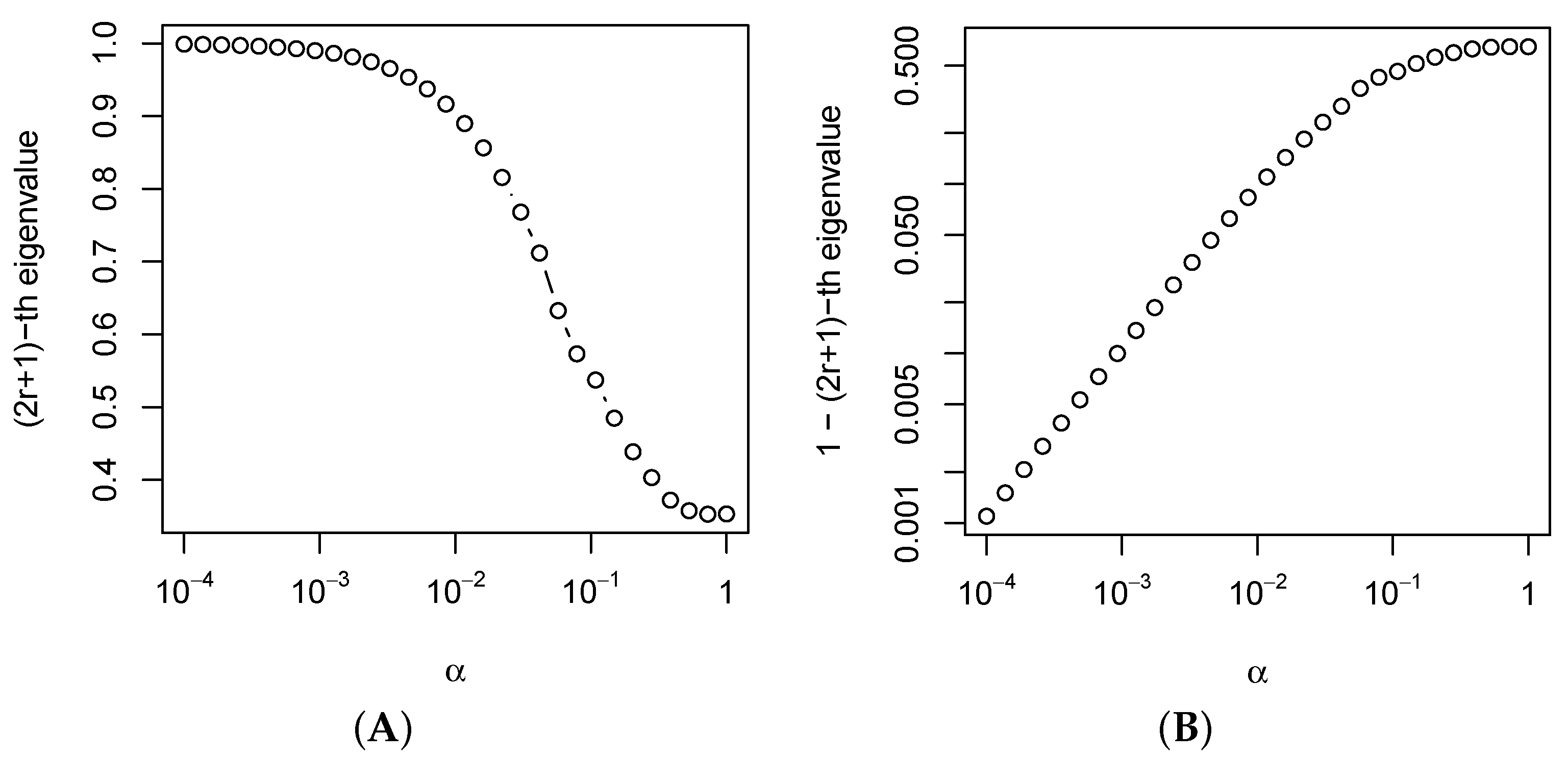
Figure 1 shows the $(2r+1)$-th eigenvalue of the ${\mathbf{P}}_{{\mathsf{S}}_0,(\mathbf{L},\mathbf{R})}$ (the squared cosine of the $(2r+1)$-th principal angle between the corresponding subspaces) for the series ${\mathsf{S}}_0={(s_1,\dots ,s_N)}^{\mathrm{T}}$ with the common term $s_k=sin\left(\frac{2\pi k}{6}\right)$ and $N=40$; the window length is $L=20$ and the signal rank is $r=2$. The values $\alpha$ are taken from $[{10}^{-4},1]$ on the logarithmic scale, and the matrix $\mathbf{R}$ is calculated using the weight search method from [14]. Figure 1 demonstrates that the eigenvalues are close to 1 for small $\alpha$; however, they do not equal one; that is, the Cadzow iterations converge. This result explains the decrease in the convergence rate of the Cadzow method with decreasing values of the parameter $\alpha$, which was numerically demonstrated in [13,14].

5. Mixed Cadzow Iterations

5.1. Convergence of Linearized Mixed Iterations

Let us introduce a linearized analogue of the mixed Cadzow algorithm (6), using the matrix ${\mathbf{P}}_{{\mathsf{S}}_0,(\mathbf{L},\mathbf{R})}$ defined in (14). Instead of (6), we will study

$${\mathsf{X}}_T={\mathbf{P}}_{{\mathsf{S}}_0,({\mathbf{L}}_2,{\mathbf{R}}_2)}^{T_2}{\mathbf{P}}_{{\mathsf{S}}_0,({\mathbf{L}}_1,{\mathbf{R}}_1)}^{T_1}{\mathsf{X}}_0,$$

(20)

where $T=T_1+T_2$. Since this formula uses only linear operators, the following theorem follows directly from Theorem 2.

Theorem 6.

Let ${\mathsf{S}}_0$ be a time series governed by the GLRR(${\mathbf{a}}_0$). The following relations are true for iterations (20), where convergence is in the operator norm:

1. 

${\mathbf{P}}_{{\mathsf{S}}_0,({\mathbf{L}}_2,{\mathbf{R}}_2)}^{T_2}{\mathbf{P}}_{{\mathsf{S}}_0,({\mathbf{L}}_1,{\mathbf{R}}_1)}^{T_1}\to {\Pi }_{\mathcal{Z}\left({\mathbf{a}}_0^2\right),{\mathbf{L}}_1\ast {\mathbf{R}}_1}$ if $T_2$ is fixed and $T_1\to +\infty$.

2. 

There is a symmetric positive-definite matrix $\mathbf{Q}\in {\mathbb{R}}^{N\times N}$ such that

${\mathbf{P}}_{{\mathsf{S}}_0,({\mathbf{L}}_2,{\mathbf{R}}_2)}^{T_2}{\mathbf{P}}_{{\mathsf{S}}_0,({\mathbf{L}}_1,{\mathbf{R}}_1)}^{T_1}\to {\Pi }_{\mathcal{Z}\left({\mathbf{a}}_0^2\right),\mathbf{Q}}$ if $T_1$ is fixed and $T_2\to +\infty$.

Thus, to achieve fast and accurate estimates, the weights $({\mathbf{L}}_1,{\mathbf{R}}_1)$ should correspond to more accurate but possibly slower-converging Cadzow iterations, and the weights $({\mathbf{L}}_2,{\mathbf{R}}_2)$ should correspond to less accurate but faster-converging iterations. The convergence rate of the corresponding operators is explained by Proposition 1. As follows from the discussion in Section 4.4, the pair of matrices $({\mathbf{L}}_1,{\mathbf{R}}_1)$ is natural to choose as an approximation of the optimal weight matrix $\mathbf{W}$ with a small parameter $\alpha$, and the pair $({\mathbf{L}}_2,{\mathbf{R}}_2)$ corresponds to a larger value $\alpha$.

5.2. Numerical Experiments

In this section, we demonstrate the result of Theorem 6 through a numerical experiment. Consider the problem of estimating a finite-rank signal when it is corrupted by noise. As in Section 4.4.2, the signal has the form ${\mathsf{S}}_0={(s_1,\dots ,s_N)}^{\mathrm{T}}$, where $s_k=sin\left(\frac{2\pi k}{6}\right)$ and $N=40$. The observed time series is $\mathsf{X}={\mathsf{S}}_0+\epsilon$, where $\epsilon$ is Gaussian white noise with zero mean and standard deviation $\sigma =0.1$.

Let us apply iterations given in (6) for estimating the signal ${\mathsf{S}}_0$. Set $L=20$ and $r=2$. Let us take $T_1$ iterations with one of three values of $\alpha$, 0.5, 0.1 and 0.01, and then $T_2$ iterations with $\alpha =1$. For the second iterations, we consider the identity matrices ${\mathbf{L}}_2$ and ${\mathbf{R}}_2$ (this choice corresponds to $\alpha =1$). For the choice of $({\mathbf{L}}_1,{\mathbf{R}}_1)$, we set ${\mathbf{L}}_1$ as the identity matrix, and for a given $\alpha$, we calculated the matrix of weights ${\mathbf{R}}_1$ using the method described in [14].

We denote the results of the iterations ${\mathbf{Y}}^{☆}$ and the signal estimate $\widehat{\mathsf{S}}={\mathcal{T}}_L^{-1}\left({\mathbf{Y}}^{☆}\right)$. For the linearized version (20), we can use the theoretical considerations. For the Cadzow mixed iterations (6), we have no theoretical results and estimated the error using $I=1000$ simulations of time series with different realizations of noise. The accuracy of the estimate was measured by RMSE (root mean square error) and estimated as the square root of the sample mean of I realizations of ${\sum }_{i=1}^N{({\widehat{s}}_i-s_i)}^2/N$.

The estimate of the signal $\mathsf{S}$ using the linearized Cadzow algorithm has the form $\tilde{\mathsf{S}}={\mathsf{S}}_0+{\Pi }_{\mathcal{Z}\left({\mathbf{a}}_0^2\right),\mathbf{Q}}\epsilon$, where ${\Pi }_{\mathcal{Z}\left({\mathbf{a}}_0^2\right),\mathbf{Q}}$ was taken from the second statement of Theorem 6 and GLRR(${\mathbf{a}}_0$) governs the signal ${\mathsf{S}}_0$. To calculate RMSE of $\tilde{\mathsf{S}}$, we consider its autocovariance matrix ${\Sigma }_{\tilde{\mathsf{S}}}={\Pi }_{\mathcal{Z}\left({\mathbf{a}}_0^2\right),\mathbf{Q}}\Sigma {\Pi }_{\mathcal{Z}\left({\mathbf{a}}_0^2\right),\mathbf{Q}}^{\mathrm{T}}$, where $\Sigma ={\mathbf{I}}_N$ is the autocovariance matrix of $\epsilon$. Then, RMSE can be calculated by taking the square root of the average value of the diagonal elements of ${\Sigma }_{\tilde{\mathsf{S}}}$, since the i-th element of the diagonal is the variance of ${\tilde{s}}_i$.

The results are shown in Figure 2. The legend denotes the values of $\alpha$ for obtaining the matrix weights ${\mathbf{R}}_1$, and which method was used (“Linear” corresponds to linearization (20), and “True” corresponds to the original Cadzow method (6)). To demonstrate the statement 2 of Theorem 6, we took a large $T_2$, which numerically corresponds to the case $T_2=\infty$.

We see that the results predicted for the linearized Cadzow iterations and estimated by simulation for the original Cadzow iterations are similar.

To demonstrate that the proposed approach allows one to improve the computational costs while keeping the accuracy high, let us consider the dependence of RMSE on $T_1+T_2$, where the total number of iterations $T_1+T_2$ changes from 1 to 10 and $\alpha =0.02$.

In Figure 3, the case $T_1=0$ (marked as “$0.02\times 0+1\times 10$”) corresponds to the case of fast convergence but low accuracy for standard Cadzow iterations with $\alpha =1$. The case $T_1=10$ (“$0.02\times 10+1\times 0$”) corresponds to the case of slow convergence but has good accuracy for Cadzow iterations with $\alpha =0.02$. The mixed iterations with two and four iterations with $\alpha =0.02$ and then iterations with $\alpha =0.1$ (“$0.02\times 2+1\times 8$” and “$0.02\times 4+1\times 6$” respectively) show their advantage in computational cost. One can see that one iteration of the second type is sufficient to almost achieve the limiting accuracy. Thereby, for example, four iterations with $\alpha =0.02$ and one iteration with $\alpha =1$ provide approximately the same accuracy and two-times faster than 10 iterations with $\alpha =0.02$.

6. Discussions

In the previous section, we demonstrated the potential advantage of mixed Cadzow iterations. The following questions arise for use in practice. The first important issue to discuss is the stability of the demonstrated effect. One source of perturbation is that the signal rank can be inaccurately estimated. Of course, if the rank is underestimated, most methods fail. The question is the robustness of the method to rank overestimation. Let us take the time series from Section 5.2 with a signal of rank 2 and consider a projection onto a subspace of rank 4 in alternating projections (target rank 4). Figure 4 shows that the general error behaviour is similar to that in Figure 3; the only differences are the convergence rate and the number of accurate steps required.

The second example is related to the stability of the result concerning the signal rank. We changed the signal from the previous example to $s_n=sin(2\pi n/6)+0.5sin(2\pi n/8)-0.3sin(2\pi n/12)$. Figure 5 demonstrates the same effect: similar behavior of the error dynamics and a lower rate of convergence. Note that the convergence for the case of rank 6 is much faster than for the overestimated rank 2.

Both examples show that the number of first accurate iterations depends on the structure of the series. Therefore, the choice of the number of accurate steps should be investigated in the future.

The next point of discussion is the possibility of speeding up the implementation of Cadzow iterations. Ideas from [21], including the randomized linear algebra approach [22,23], can be applied to Cadzow iterations. Combining the mixed alternating projection approach and approaches to single iteration acceleration may be a challenge for future research.

7. Conclusions

In this paper, an approach for improving the alternating projection method by combining the alternating projections in two equivalent norms was proposed and justified. The approach in general form was considered for the case of projections to linear subspaces (Theorem 2). Then, this approach was applied to the problem of Hankel low-rank approximation, which is considered for the estimation of low-rank signals and is not linear. The theoretical results were obtained using the linearization (13). Numerical experiments confirmed that the linearization provides the correct conclusions for the convergence of the mixed Cadzow iterations (6). Using the theory of principal angles, it was shown why improving the estimation accuracy leads to increasing the computational cost of the conventional Cadzow iterations (Section 4.4). Using the features of the projector compositions, it was shown how the signal estimation can be improved by a combination of iterations with different norms (Theorem 6).

As a result, the algorithm, which modifies the Cadzow weighted iterations by combining a good accuracy of slow iterations and a fast convergence of inaccurate iterations, was proposed.

The numerical example in Section 5.2 demonstrates the effectiveness of the elaborated approach. The examples are implemented in R using the R-package rhlra, which can be found at https://github.com/furiousbean/rhlra (accessed on 13 October 2022); see the R-code of the examples in Supplementary Materials.