A Mask-Based Adversarial Defense Scheme

Abstract

Adversarial attacks hamper the functionality and accuracy of deep neural networks (DNNs) by meddling with subtle perturbations to their inputs. In this work, we propose a new mask-based adversarial defense scheme (MAD) for DNNs to mitigate the negative effect from adversarial attacks. Our method preprocesses multiple copies of a potential adversarial image by applying random masking, before the outputs of the DNN on all the randomly masked images are combined. As a result, the combined final output becomes more tolerant to minor perturbations on the original input. Compared with existing adversarial defense techniques, our method does not need any additional denoising structure or any change to a DNN’s architectural design. We have tested this approach on a collection of DNN models for a variety of datasets, and the experimental results confirm that the proposed method can effectively improve the defense abilities of the DNNs against all of the tested adversarial attack methods. In certain scenarios, the DNN models trained with MAD can improve classification accuracy by as much as $90\%$ compared to the original models when given adversarial inputs.

1. Introduction

Deep neural networks (DNNs) have achieved great success in the past decade in research areas such as image classification, natural language processing, and data analytics, with a variety of application domains like banking, financial services and insurance, IT and telecommunications, manufacturing, and healthcare etc. [1]. However, researchers have discovered that it is possible to introduce human imperceptible perturbations to inputs of a DNN in order to induce incorrect or misleading outputs from the DNN at the choice of an adversary [2,3,4].

As of today, the existing approaches to counter adversarial attacks can be roughly divided into two categories. The reactive approach focuses on the detection of adversarial inputs (e.g., [5,6,7]) and tries to correct the adversarial inputs. The proactive approach, sometimes known as adversarial defense, takes steps to strengthen DNNs (e.g., [8,9,10]), making them more robust to withstand perturbations on inputs. In this paper, we follow the latter path by enhancing robustness in the decision procedure of DNNs. Inspired by a recent paper [11] that restores missing pixels of provided images with random patching, we devise a new adversarial defense scheme called mask-based adversarial defense (MAD) for the training and testing of DNNs that perform image-classification tasks. In addition, we believe that such a mechanism may also be applicable to improve DNN robustness in other scenarios.

In this approach, we perform a series of experiments with regard to MAD. We split an image into grids of predefined size (e.g., $4\times 4$), and randomly fill each grid by using a default value (e.g., the black value in RGB for those masked pixels) with a given probability (e.g., $75\%$) to generate training samples. After the training, we also apply masking to images at the test phase (for the classification task), as illustrated in Figure 1. Given an (unmasked original) image, we need to repeat the test process a number of times with different patterns of masking, which increases the chance of filtering out malicious perturbations, and the final decision is then defined as the most-voted class taking into account the outputs for all randomly masked inputs. In this paper, we have made the following contributions.

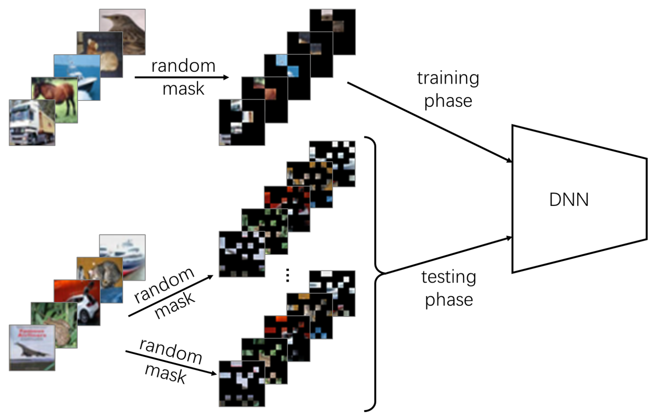
• We introduce a new adversarial defense method, MAD. Our method applies randomized masking at both training phase and test phase, which makes it resistant to adversarial attacks.
• Our method seems easily applicable to many existing DNNs. Compared with other adversarial defense methods, we do not need special treatment for the structures of DNNs, redesign of loss functions, or any (autoencoder-based) input filtering.
• The experiment on a variety of models (LeNet, VGG, and ResNet) has shown the effectiveness of our method with a significant improvement in defense (up to $93\%$ precision gain) when facing various adversarial samples, compared to models not trained with MAD.

2. Related Work

Because we work on an adversarial defense scheme, we conduct a brief survey on the adversarial attack methods and various types of adversarial defense methods.

2.1. Adversarial Attack

In general, an adversarial attack method generates tiny perturbations that are applied to clean inputs, making them incorrectly classified by a DNN. Some of the earliest methods include box-constrained L-BFGS [2], fast gradient sign method (FGSM) [3] and Jacobian-based saliency map attack (JSMA) [12]. Perhaps the most widely used adversarial attack is FGSM, which is also included as an attack method in our experiment. FGSM generates a perturbation for an image by computing the following,

$$\delta =ϵsign\left({▿}_{x}L(\theta ,x,y)\right),$$

(1)

where $L(·)$ is the loss function used for neural network training which calculates the difference between expected output value and the output produced from input x for the DNN with parameter $\theta$. The direction of movement is obtained by the gradient of loss and constant $ϵ$ which restricts the norm of perturbation. The basic iterative method (BIM) [13] and projected gradient descent (PGD) [9] are the iteration and extension of FGSM to obtain better attack effect, respectively.

Here we focus on DNNs that classify images. Formally, a DNN is a function $f_{\theta }$ which maps $\mathcal{X}\subseteq {\mathbb{R}}^d$ to $\mathcal{Y}$, where $\theta$ represents values for the network parameters that are determined at training, d is the dimension of the input space, $\mathcal{X}$ is the input space for images and $\mathcal{Y}$ is a finite set of classes or labels to be returned from $f_{\theta }$. An adversarial input can be written as $x^{\prime }=x+\delta$ with x a clean input and ${\left|\right|\delta \left|\right|}_p<\epsilon$, such that $f_{\theta }\left(x\right)\ne f_{\theta }\left(x^{\prime }\right)$, where ${\left|\right|\delta \left|\right|}_p$ is the p norm of the perturbation $\delta$ and $\epsilon >0$ is of negligible size, making x and $x^{\prime }$ in the same class as a human being.

2.2. Adversarial Defense

Adversarial defense aims to counter the adversarial effect and make DNNs achieve a performance on adversarial samples close to results on clean samples. Existing approaches can be roughly classified as (1) use of additional denoising structures before the DNN, and (2) enforcing the DNN to become more robust against adversarial attacks.

Additional denoising structures. The reactive approach focuses on the detection of adversarial inputs (e.g., [5,6,7]) and tries to "correct" the adversarial inputs. MagNet [8] is a framework consisting of a detector that rejects adversarial samples that are far away from the normal input manifolds, and a reformer that finds the closest normal input if the adversarial input is not far from the manifolds. A similar approach is HGD [14], which applies a high-level representation-guided denoiser, so that it can be designed as a defense model that transforms adversarial inputs to easy-to-classify inputs. The defense-GAN [15] tries to model the distribution of clean images, and it can find a close output to an adversarial image which does not contain the adversarial changes. Denoised smoothing [16] prepends a custom-trained denoiser to a DNN and uses randomized smoothing for training the combination which enforces a nonlinear Lipschitz property. PixelDefend [17] approximates the training distribution by using a PixelCNN model and purifies images toward higher probability areas of the training distribution. Compared with our method, all these approaches introduce additional network structures that help to remove adversarial noise from inputs at the cost of increasing the number of parameters of the working model. In our experiment, we also empirically show that MAD outperforms MagNet and denoised smoothing in most of the test cases.

DNN model enhancement. The proactive approach, sometimes known as adversarial defense, takes steps to strengthen DNNs (e.g., [8,9,10]), making them more robust to withstand perturbations on inputs. In this category, adversarial training [9,18] and defensive distillation [4] are among the early successful approaches. In particular, adversarial training introduces adversarial samples at the training phase to enhance resistance against attacks. Defensive distillation transfers a DNN to another with the same functionality but is less sensitive to input perturbations. However, both adversarial training and defensive distillation require substantially more training cost. Introducing randomized variation to inputs and network parameters at the time of training as been discussed in [19,20]. Parseval networks [21] limit the Lipschitz constant of linear, convolutional, and aggregation layers in the network to be smaller than 1, making these layers tight frames. PCL [10] separates the hidden feature of different categories by designing a new loss function and bypass network, so as to increase the difficulty of adversarial attacks and achieve the effect of adversarial defense. Because the existing DNN models are already being optimized with regard to performance (e.g., neural network search (NAS) [22] technology is widely used to find neural networks structure with better performance), the modification of DNN structures may introduce human bias, resulting in unpredictable performance degradation. In contrast, our approach MAD does not require any change to network structure or loss function design.

3. Materials and Methods

3.1. Training a Classifier for Masked Images

A natural approach to counter an adversarial input $x^{\prime }$ is to reduce the effect of perturbation $\delta$. Given $\delta$ combined with the pixels of a natural image x, masking part of $x^{\prime }$ would potentially reduce the adversarial effect of $\delta$. Fortunately, such a masking operation which ”masks” some parts of an image does not necessarily make the classification job more difficult for DNNs. Because natural images are heavy in spatial information redundancy, as shown in [11], in which missing pixels of an image can be reconstructed by the state-of-the-art MAE model even though a large amount of input pixels are masked. Our human brains possess the similar power of recognizing (or even reconstructing) a partially masked object. Because the task of image classification is supposed to be easier than image reconstruction, this leads us to the first step of training a DNN classifier for masked images, keeping the same network structure as the original DNN to be defended.

In the proposed method, images are partially masked in both the training phase and the test phase. For our experiment, in the training phase, each image from the training samples of CIFAR-10 [23] and SVHN [24] is divided into $8\times 8$ grids, and images from MNIST [25] are divided into $7\times 7$ grids, so that the length of a grid always divides the length of an image (CIFAR-10 and the SVHN datasets contain $32\times 32$ images and the MNIST dataset contains $28\times 28$ images).

We then conduct a preliminary study on the retrained VGG16 [26] classifier for masked images from CIFAR-10, and the results are shown in Figure 2. In this study, we combine results from multiple tests of the same image with randomized masking applied, and the most-occurred class of all test results is returned as the output for that image. The original VGG16 model (i.e., $f_{\theta }$) has $84.18\%$ accuracy on the test data. The retrained model (i.e., $f_{{\theta }^{\prime }}$) is obtained by letting each $8\times 8$ grid have $3/4$ probability to be masked for training inputs, and similarly, test images also have $3/4$ probability for each $4\times 4$ grid to be masked. It can be easily seen that applying masking on images with a single test does imply performance degradation ($75.89\%$ for $f_{{\theta }^{\prime }}$ dropped from $84.18\%$ for $f_{\theta }$). However, it seems that the loss of precision can be partially remedied by applying multiple tests on the same image, as one may find that in the case of combining 7 tests, a precision of $82.97\%$ can be achieved. The time required for the tests increases linearly with the increase of the number of masked images generated for each original input, as shown by the green line in Figure 2. Even if each image is repeatedly tested 7 times, in our experiment, the test speed of 296fps can be achieved on single NVIDIA GeForce RTX 3090 GPU when running the test.

3.2. Mitigating Adversarial Attacks

In our second step, we investigate how the new model trained for masked images can be used to boost defense against adversarial inputs. Given an adversarial input $x^{\prime }=x+\delta$, the new model produces $f_{{\theta }^{\prime }}\left(\tau (x+\delta ,c)\right)$ with a randomly picked mask parameter c. Let ${\delta }^{\prime }=\tau (x+\delta ,c)-\tau (x,c)$, which is the actual perturbation (vector) on the input to $f_{{\theta }^{\prime }}$, and it is obvious that we have $\left|\right|{\delta }^{\prime }{\left|\right|}_p\le {\left|\right|\delta \left|\right|}_p$ for any p and any c, since only unmasked pixels of x are affected by $\delta$. As an example, suppose $3/4$ of the input pixels are masked, the expected ${\ell }_1$ norm of ${\delta }^{\prime }$ is only about $1/4$ in size of the ${\ell }_1$ norm of the original perturbation $\delta$.

In order to measure how much the effect of adversarial inputs is weakened by masking, we conduct another preliminary study by randomly removing part of the perturbation vector $\delta$ from an adversarial input. We first train a VGG16 model on CIFAR-10 data set by using the conventional method. Then, given adversarial samples generated from clean samples, we obtain each perturbation vector by taking the difference between an adversarial input and its corresponding clean image. These vectors are then randomly masked before adding back to the clean images to form a set of weakened attack samples. The relationship between the model accuracy and the proportion of the remaining adversarial disturbance is shown in Figure 3, where $100\%$ remaining adversarial disturbance represents strength of the original adversarial inputs, and $20\%$ remaining represents the adversarial inputs with $80\%$ of the perturbation dimensions removed. In particular, we find that the CW attack is more sensitive to this perturbation removal operation, which may be due to the fact that CW generates smaller perturbation with higher relevance. For most other attacks, we find that removing at least $60\%$ of the perturbation (i.e., at most $40\%$ of the attack perturbation remaining) is required to deliver significant improvement regarding classification accuracy.

In general, there is often a tradeoff between the strength of defense and the degree of accuracy. As shown in

Table 1. Defense of different mask rates with the grid size of $8\times 8$ for the training phase and $4\times 4$ for the test phase, on a VGG16 model with CIFAR-10 dataset.

Attack Method	0	$1/3$	$1/2$	$3/4$	$4/5$
Benign	84.18%	85.31%	84.59%	82.65%	76.14%
FGSM L1 $ϵ$ = 15	63.53%	70.17%	78.37%	82.63%	85.30%
FGSM L1 $ϵ$ = 20	63.01%	64.82%	73.70%	79.25%	82.14%
FGSM L2 $ϵ$ = 0.3	67.36%	75.95%	82.46%	84.62%	87.55%
FGSM L2 $ϵ$ = 0.4	66.23%	70.18%	78.33%	81.89%	84.66%
FGSM Linf $ϵ$ = 0.01	48.88%	68.87%	76.07%	81.05%	83.74%
FGSM Linf $ϵ$ = 0.02	40.76%	53.77%	61.30%	68.77%	70.61%
BIM L1 $ϵ$ = 10	59.02%	67.66%	79.63%	84.71%	87.88%
BIM L1 $ϵ$ = 15	58.23%	51.27%	68.89%	80.91%	84.91%
BIM L2 $ϵ$ = 0.3	61.86%	61.60%	75.69%	83.21%	87.04%
BIM L2 $ϵ$ = 0.4	61.57%	49.33%	68.02%	80.88%	84.25%
BIM Linf $ϵ$ = 0.01	38.29%	57.77%	72.21%	81.80%	86.14%
BIM Linf $ϵ$ = 0.015	37.15%	39.75%	58.60%	77.06%	82.61%
PGD L1 $ϵ$ = 1	58.49%	64.60%	79.17%	85.44%	88.11%
PGD L1 $ϵ$ = 20	57.69%	54.85%	73.67%	83.48%	86.89%
PGD L2 $ϵ$ = 0.3	62.30%	71.87%	82.82%	86.42%	89.19%
PGD L2 $ϵ$ = 0.4	61.63%	62.71%	77.28%	84.45%	87.83%
PGD Linf $ϵ$ = 0.01	40.29%	65.37%	77.61%	84.78%	88.26%
PGD Linf $ϵ$ = 0.015	37.16%	49.63%	67.64%	81.45%	85.63%
CW L2 $ϵ$ = 1	63.11%	95.46%	95.87%	91.28%	93.24%
DeepFool L2 $ϵ$ = 0.6	53.97%	74.01%	80.90%	84.20%	87.22%
DeepFool L2 $ϵ$ = 0.8	52.61%	68.15%	76.07%	81.19%	83.86%
DeepFool Linf $ϵ$ = 0.01	50.70%	75.72%	82.95%	85.23%	87.59%
DeepFool Linf $ϵ$ = 0.015	44.32%	67.31%	75.12%	80.44%	83.81%

of our experiment in the next section, after fixing a network structure, increasing the percentage of masked pixels (at both the training and test phases) often results in a stronger defense against most of the tested adversarial attacks, but with less accurate classification results on benign (clean) inputs. For example, given the first FGSM attack with perturbation degree 15, setting a mask rate of $1/3$ yields a model with defense accuracy of $70.17\%$ on adversarial samples, which is less effective compared to the $85.3\%$ accuracy when each grid has a $4/5$ probability of being masked. However, the $4/5$ masked model only has $76.14\%$ accuracy on benign images, whereas the $1/3$ masked model has $85.31\%$ accuracy.

3.3. Basic Settings for Adversarial Attack and Defense

The experiments are based on TensorFlow 2.6 and completed on a server running Ubuntu 18.04LTS with a NVIDIA GeForce RTX 3090 GPU. The Adam optimizer is used in the training phase with a learning rate $0.001$. We choose three popular DNN models (LeNet with MNIST [25], VGG16 [26] with CIFAR-10 [23], and ResNet18 [27] with SVHN [24]). In order to achieve a classification accuracy close to its corresponding DNN model on benign (clean) images, for each original image input, we take the most favored class of all 5 tests as the output prediction.

Foolbox [28] is used to generate adversarial samples for the test set. We leave the parameters of all adversarial attack methods as their default settings, except for the perturbation degree $ϵ$, which is specified in the “Attack method” column of the tables. Note that for all experiments in this paper, adversarial samples are generated only from benign images that are correctly classified by the DNNs. The adversarial attack algorithms also take into account the parameters of the MAD model. The generated adversarial samples aim to lower the accuracy of the MAD model without masking, e.g., the FGSM L1 with $ϵ=10$ attack results in the original LeNet model with $44.12\%$ accuracy. When multiple randomized masking is applied at testing, the accuracy of the MAD model becomes $68.94\%$ (with $24.82\%$ improvement) facing adversarial samples. In this process, we generate adversarial images directly to attack the MAD model without masking. We believe this is a reasonable setting as an attacker would not be able to know which grids from an original input image are to be masked ahead of time, and the possible ways of random masking to a given input are exponential in size of the image (i.e., $2^{\left|G\right|}$ where $\left|G\right|$ is the number of grids, which is linear in size of the input). Although it is possible that all grids are masked and all information is lost from input, this is in general regarded as unlikely to happen, and most randomly masked images have their actual mask rates close to the set value, which is $3/4$ in most of the experiments in the paper. Our discussion on the choice of mask rate is given in Section 4.2.

For our experiment on the comparison, the implementations of denoised smoothing https://github.com/microsoft/denoised-smoothing (accessed on 9 November 2022) and PCL https://github.com/aamir-mustafa/pcl-adversarial-defense (accessed on 9 November 2022) are publicly available from their respective authors, and the codes for the MagNet and Parseval networks are available from a third party, Gokul Karthik https://github.com/GokulKarthik/MagNet.pytorch (accessed on 9 November 2022) and the Python library parsnet https://github.com/mathialo/parsnet (accessed on 9 November 2022), respectively.

4. Results

4.1. Ablation Study

The ablation study focuses on the effect of masking on both the training phase and the test phase. There are four choice combinations are (1) no masking being applied, (2) to apply masking only at the training phase, (3) to apply masking only at the test phase, and (4) to apply masking both at the training phase and the test phase. We choose the model VGG16 for the CIFAR-10 data set, $3/4$ as the mask rate, $8\times 8$ grids for training and $4\times 4$ grids for testing. We use a benign sample together with adversarial samples generated from BIM Linf ($ϵ=0.01$), PGD Linf ($ϵ=0.01$), CW L2 ($ϵ=1.0$), and DeepFool Linf ($ϵ=0.01$) algorithms.

Table 2. Defense effect of using masked and nonmasked images during training and testing.

Masked		Classification Accuracy
Training	Testing	Benign	BIM Linf $\mathbf{ϵ}$ = 0.01	PGD Linf $\mathbf{ϵ}$ = 0.01	CW L2 $\mathbf{ϵ}$ = 1.0	DeepFool Linf $\mathbf{ϵ}$ = 0.01
×	×	84.18%	38.29%	40.29%	63.11%	50.70%
√	×	84.65%	3.16%	6.13%	15.89%	35.72%
×	√	49.39%	67.98%	69.37%	70.06%	67.98%
√	√	82.65%	81.80%	84.78%	91.28%	85.23%

shows the results of the ablation experiment. We find that the model with masking applied at both the training phase and the test phase greatly outperforms other combinations when facing adversarial samples. In the case of the clean sample, applying masking at both phases still have an acceptable precision of $82.65\%$, close to the best performance of $84.65\%$ where masking is only applied at training.

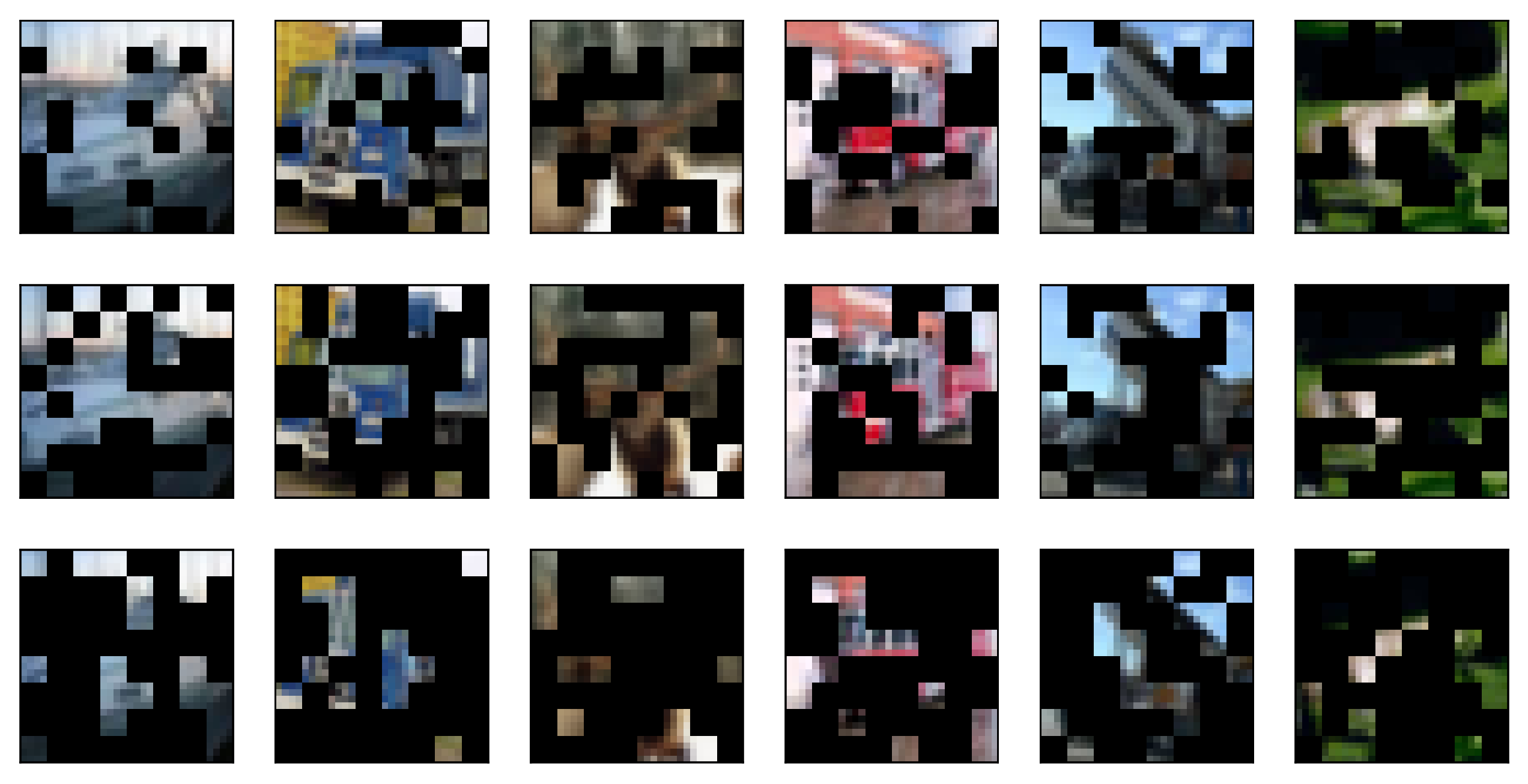
4.2. On Mask Rates and Grid Sizes

The effectiveness of MAD also depends on two critical hyperparameters. The mask rate is a constant which is used as the probability for a grid to be masked at the training phase as well as test phase. As mentioned before, a larger mask rate potentially removes more perturbation (which means better defense) at the cost of less usable information for the classifier, which may lead to worse accuracy on clean images.

We carry out an experiment on a selection of mask rates ($1/3$, $1/2$, $3/4$, $4/5$, sample images illustrated in Figure 4) with grid size fixed at $8\times 8$ for the training phase and $4\times 4$ for the test phase, on a VGG16 model with image data from CIFAR-10. The experimental results are shown in Table 1. It can be seen from the results that a higher masking percentage makes a better defense but has lower accuracy on benign inputs. Considering that in a real-life scenario, a DNN may receive a mixed set of benign and adversarial inputs, say $1/2$ benign samples and $1/2$ adversarial samples, for the mask rate of $3/4$ and adversarial samples generated by FGSM with $ϵ=15$, the real-life defense score can then be calculated as the weighted average $\frac{1}{2}\times 82.63\%+\frac{1}{2}\times 82.65\%=82.64\%$ as a fair guess in this hypothetical scenario (data as from the top two rows at column $3/4$ of Table 1). Therefore, we believe that $3/4$ could be a reasonable mask rate, which yields acceptable accuracy for both benign and adversarial inputs, and we use it for all experiments conducted in rest of the paper.

The grid size is another hyperparameter to be determined before the main experiment. Intuitively, a larger grid size allows better continuity of information on average that is preserved in a masked image (examples illustrated in Figure 5).

Table 3. Defense effects of different grid sizes with mask rate of 3/4 on VGG16 and CIFAR-10 dataset.

Training	4 × 4	4 × 4	8 × 8	8 × 8	8 × 8
Test	2 × 2	4 × 4	2 × 2	4 × 4	8 × 8
Benign	73.23%	76.92%	63.11%	82.65%	82.89%
FGSM L1 $ϵ$ = 15	86.63%	83.84%	85.34%	82.63%	75.68%
FGSM L1 $ϵ$ = 20	83.20%	79.39%	82.74%	79.25%	71.72%
FGSM L2 $ϵ$ = 0.3	89.54%	87.13%	86.17%	84.62%	79.84%
FGSM L2 $ϵ$ = 0.4	86.63%	83.41%	85.34%	81.89%	75.11%
FGSM Linf $ϵ$ = 0.01	86.10%	82.11%	84.42%	81.05%	73.63%
FGSM Linf $ϵ$ = 0.02	73.64%	67.07%	73.93%	68.77%	59.87%
BIM L1 $ϵ$ = 10	89.21%	85.66%	87.64%	84.71%	75.67%
BIM L1 $ϵ$ = 15	84.62%	79.36%	85.61%	80.91%	65.50%
BIM L2 $ϵ$ = 0.3	87.52%	83.55%	86.12%	83.21%	71.88%
BIM L2 $ϵ$ = 0.4	83.64%	78.06%	85.50%	80.88%	65.82%
BIM Linf $ϵ$ = 0.01	86.60%	81.86%	86.47%	81.80%	68.67%
BIM Linf $ϵ$ = 0.015	81.26%	72.97%	83.62%	77.06%	56.05%
PGD L1 $ϵ$ = 15	88.99%	84.76%	86.64%	85.44%	76.14%
PGD L1 $ϵ$ = 20	85.78%	80.08%	86.23%	83.48%	71.13%
PGD L2 $ϵ$ = 0.3	90.35%	87.03%	88.07%	86.42%	78.77%
PGD L2 $ϵ$ = 0.4	88.01%	83.48%	87.20%	84.45%	74.79%
PGD Linf $ϵ$ = 0.01	88.64%	84.05%	86.61%	84.78%	73.89%
PGD Linf $ϵ$ = 0.015	84.57%	77.20%	84.46%	81.45%	65.54%
CW L2 $ϵ$ = 1	94.78%	95.25%	89.53%	91.28%	93.94%
DeepFool L2 $ϵ$ = 0.6	88.54%	87.10%	85.03%	84.20%	80.31%
DeepFool L2 $ϵ$ = 0.8	85.73%	82.75%	82.65%	81.19%	75.53%
DeepFool Linf $ϵ$ = 0.01	90.33%	88.21%	85.42%	85.23%	80.42%
DeepFool Linf $ϵ$ = 0.015	86.03%	82.66%	82.16%	80.44%	74.92%

presents the preliminary experimental results on a VGG model with CIFAR-10 dataset for a selection of grid size values in the masking operation at the time of training and testing, respectively. Given images in CIFAR-10 are of size $32\times 32$, we try a number of combinations for values that divide 32. If we focus on the three columns where $8\times 8$ grids are used for training, the results seem to suggest that using a larger grid in the test phase produces a better classification accuracy on benign images, and a smaller grid produces a better defense. We choose $8\times 8$ (training) and $4\times 4$ (testing) for the VGG16 model and CIFAR-10 dataset, and adopt this same setting for ResNet and SVHN, which also use $32\times 32$ images. For the LeNet model and MNIST dataset ($28\times 28$ images), we use $7\times 7$ grids for both training and testing.

4.3. The Main Result and Comparison

The main experiment is conducted on three different models: LeNet with MNIST dataset, VGG16 with CIFAR-10, and ResNet18 with SVHN, with the results presented in

Table 4. Defense against adversarial attacks by MAD on VGG16 and CIFAR-10 dataset.

Attack Method	Attack	Defense	Improvement
Benign		82.65%
FGSM L1 $ϵ$ = 15	35.48%	82.63%	47.15%
FGSM L1 $ϵ$ = 20	33.02%	79.25%	46.23%
FGSM L2 $ϵ$ = 0.3	38.29%	84.62%	46.33%
FGSM L2 $ϵ$ = 0.4	35.27%	81.89%	46.62%
FGSM Linf $ϵ$ = 0.01	33.02%	81.05%	48.03%
FGSM Linf $ϵ$ = 0.02	28.27%	68.77%	40.50%
BIM L1 $ϵ$ = 10	10.23%	84.71%	74.48%
BIM L1 $ϵ$ = 15	6.70%	80.91%	74.21%
BIM L2 $ϵ$ = 0.3	9.43%	83.21%	73.78%
BIM L2 $ϵ$ = 0.4	8.06%	80.88%	72.82%
BIM Linf $ϵ$ = 0.01	3.16%	81.80%	78.64%
BIM Linf $ϵ$ = 0.015	1.06%	77.06%	76.00%
PGD L1 $ϵ$ = 15	8.75%	85.44%	76.69%
PGD L1 $ϵ$ = 20	6.36%	83.48%	77.12%
PGD L2 $ϵ$ = 0.3	12.47%	86.42%	73.95%
PGD L2 $ϵ$ = 0.4	9.01%	84.45%	75.44%
PGD Linf $ϵ$ = 0.01	6.13%	84.78%	78.65%
PGD Linf $ϵ$ = 0.015	2.30%	81.45%	79.15%
CW L2 $ϵ$ = 1	15.89%	91.28%	75.39%
DeepFool L2 $ϵ$ = 0.6	34.64%	84.20%	49.56%
DeepFool L2 $ϵ$ = 0.8	31.81%	81.19%	49.38%
DeepFool Linf $ϵ$ = 0.01	35.72%	85.23%	49.51%
DeepFool Linf $ϵ$ = 0.015	32.26%	80.44%	48.18%

and

Table 5. Defense against adversarial attacks by MAD for LeNet (with the MNIST dataset) and ResNet18 (with the SVHN dataset).

	LeNet + MNIST				ResNet18 + SVHN
Attack Method	$\mathbf{ϵ}$	Attack	Defense	Improvement	$\mathbf{ϵ}$	Attack	Defense	Improvement
Benign	-		96.13%		-		91.65%
FGSM L1	10	44.12%	68.94%	24.82%	15	50.47%	76.84%	26.37%
FGSM L1	20	28.35%	49.50%	21.15%	20	45.85%	70.25%	24.40%
FGSM L2	0.8	34.85%	58.60%	23.75%	0.4	53.17%	80.40%	27.23%
FGSM L2	1.0	30.28%	52.82%	22.54%	0.6	46.77%	71.48%	24.71%
FGSM Linf	0.03	36.26%	61.82%	25.56%	0.01	57.12%	85.40%	28.28%
FGSM Linf	0.04	28.58%	50.31%	21.73%	0.02	46.06%	68.95%	22.89%
BIM L1	4	8.98%	59.49%	50.51%	10	15.46%	80.37%	64.91%
BIM L1	6	2.26%	44.17%	41.91%	12	11.54%	75.85%	64.31%
BIM L2	0.2	16.55%	69.23%	52.68%	0.25	21.75%	84.40%	62.65%
BIM L2	0.3	3.79%	49.04%	45.25%	0.3	16.59%	81.37%	64.78%
BIM Linf	0.015	11.72%	70.94%	59.22%	0.01	16.06%	86.31%	70.25%
BIM Linf	0.02	3.62%	56.33%	52.71%	0.02	2.58%	71.00%	68.42%
PGD L1	4	16.04%	71.79%	55.75%	14	15.09%	84.14%	69.05%
PGD L1	6	3.37%	54.75%	51.38%	16	12.11%	82.35%	70.24%
PGD L2	0.2	22.98%	77.87%	54.89%	0.4	16.40%	84.22%	67.82%
PGD L2	0.4	1.26%	48.85%	47.59%	0.5	12.17%	81.37%	69.20%
PGD Linf	0.015	11.64%	70.90%	59.26%	0.01	10.10%	84.45%	74.35%
PGD Linf	0.02	3.27%	56.38%	53.11%	0.02	4.69%	80.51%	75.82%
CW L2	1.5	0.20%	93.39%	93.19%	1.8	21.70%	96.05%	74.35%
DeepFool L2	0.6	32.62%	61.05%	28.43%	0.5	59.78%	87.09%	27.31%
DeepFool L2	0.8	26.49%	51.39%	24.90%	0.7	53.87%	82.22%	28.35%
DeepFool Linf	0.05	24.77%	47.26%	22.49%	0.01	57.10%	88.06%	30.96%
DeepFool Linf	0.07	22.50%	39.76%	17.26%	0.02	46.39%	72.98%	26.59%

. Of all the attacks, CW [29] is the most successfully defended method by MAD. One possible explanation is that CW usually produces smaller and highly correlated perturbation, which can be more easily countered by masking, as discussed in the preliminary study and presented in Figure 3. For the attack methods with different perturbation degrees ($ϵ$), MAD tends to achieve better defense on the attack methods with smaller $ϵ$, which is not surprising.

We have noticed that some works [30] use the method of random ablation to process images, which is similar to using 1 × 1 grid to mask images. We proved in Section 4.2 and Figure 3 that this method will greatly reduce the accuracy of classification. We compare MAD with four state-of-the-art adversarial defense methods, including MagNet [8], Denoised smoothing [16], Parseval networks [21], and PCL [10] on the same backbone VGG16 model with default settings, and all are tested with adversarial samples that are generated from CIFAR-10. Note that the adversarial samples used for comparison are generated only from correctly classified benign samples. None of these defense methods uses adversarial samples in the training phase. The results are shown in

Table 6. Comparison of effects of MAD with different adversarial defense methods on VGG16 with the dataset CIFAR-10.

Attack Method	MagNet	Denoised Smoothing	Parseval Networks	PCL	MAD
Benign	82.32%	77.92%	77.89%	83.47%	82.65%
FGSM L1 $ϵ$ = 15	67.41%	81.97%	43.20%	74.94%	82.63%
FGSM L1 $ϵ$ = 20	65.68%	76.50%	33.11%	70.53%	79.25%
FGSM L2 $ϵ$ = 0.3	72.15%	85.88%	52.41%	79.54%	84.62%
FGSM L2 $ϵ$ = 0.4	69.75%	81.70%	42.69%	75.32%	81.89%
FGSM Lin $ϵ$ = 0.01	57.81%	82.83%	44.22%	75.56%	81.05%
FGSM Lin $ϵ$ = 0.02	44.96%	65.25%	20.75%	62.72%	68.77%
BIM L1 $ϵ$ = 10	66.56%	80.11%	45.23%	64.03%	84.71%
BIM L1 $ϵ$ = 15	62.63%	68.58%	26.22%	48.03%	80.91%
BIM L2 $ϵ$ = 0.3	67.63%	77.36%	38.57%	61.26%	83.21%
BIM L2 $ϵ$ = 0.4	65.73%	68.06%	24.96%	48.34%	80.88%
BIM Linf $ϵ$ = 0.01	51.34%	75.51%	29.54%	59.83%	81.80%
BIM Linf $ϵ$ = 0.015	42.84%	62.41%	13.52%	43.31%	77.06%
PGD L1 $ϵ$ = 15	67.08%	79.83%	37.84%	66.63%	85.44%
PGD L1 $ϵ$ = 20	64.66%	72.81%	24.64%	53.18%	83.48%
PGD L2 $ϵ$ = 0.3	71.98%	84.65%	48.20%	76.08%	86.42%
PGD L2 $ϵ$ = 0.4	69.44%	79.17%	35.14%	66.70%	84.45%
PGD Linf $ϵ$ = 0.01	56.92%	81.17%	36.89%	72.22%	84.78%
PGD Linf $ϵ$ = 0.015	47.79%	70.74%	19.35%	54.74%	81.45%
CW L2 $ϵ$ = 1	92.58%	99.74%	43.42%	89.48%	91.28%
DeepFool L2 $ϵ$ = 0.6	63.84%	65.04%	34.10%	49.95%	84.20%
DeepFool L2 $ϵ$ = 0.8	60.45%	57.97%	44.51%	47.68%	81.19%
DeepFool Linf $ϵ$ = 0.01	62.79%	81.43%	30.49%	58.80%	85.23%
DeepFool Linf $ϵ$ = 0.015	54.26%	71.68%	9.49%	53.28%	80.44%

.

In order to make the comparison more comprehensive and more convincing, the selected defense methods have inherently different underlying defense approaches. MagNet and denoised smoothing apply additional denoising structures to reduce the adversarial perturbations. Parseval network restricts the layers’ Lipschitz constant to be less than 1 during the training, in order to boost robustness of a model. PCL enforces hidden layer features of different classes to be apart as much as possible during the training, which is imposed by adding new branch structures and introducing a new loss function.

From the results in Table 6, all methods have an acceptable accuracy on benign inputs. Nevertheless, regarding the list of tested adversarial attacks, MAD outperforms these state-of-the-art defense approaches in most cases.

5. Discussion

In this paper, we have proposed a new mask-based adversarial defense method called MAD, and have conducted extensive experiments showing that our method provides an effective defense against a variety of adversarial attacks.

First, the following observations provide a sketch of our strategy for adversarial defense.

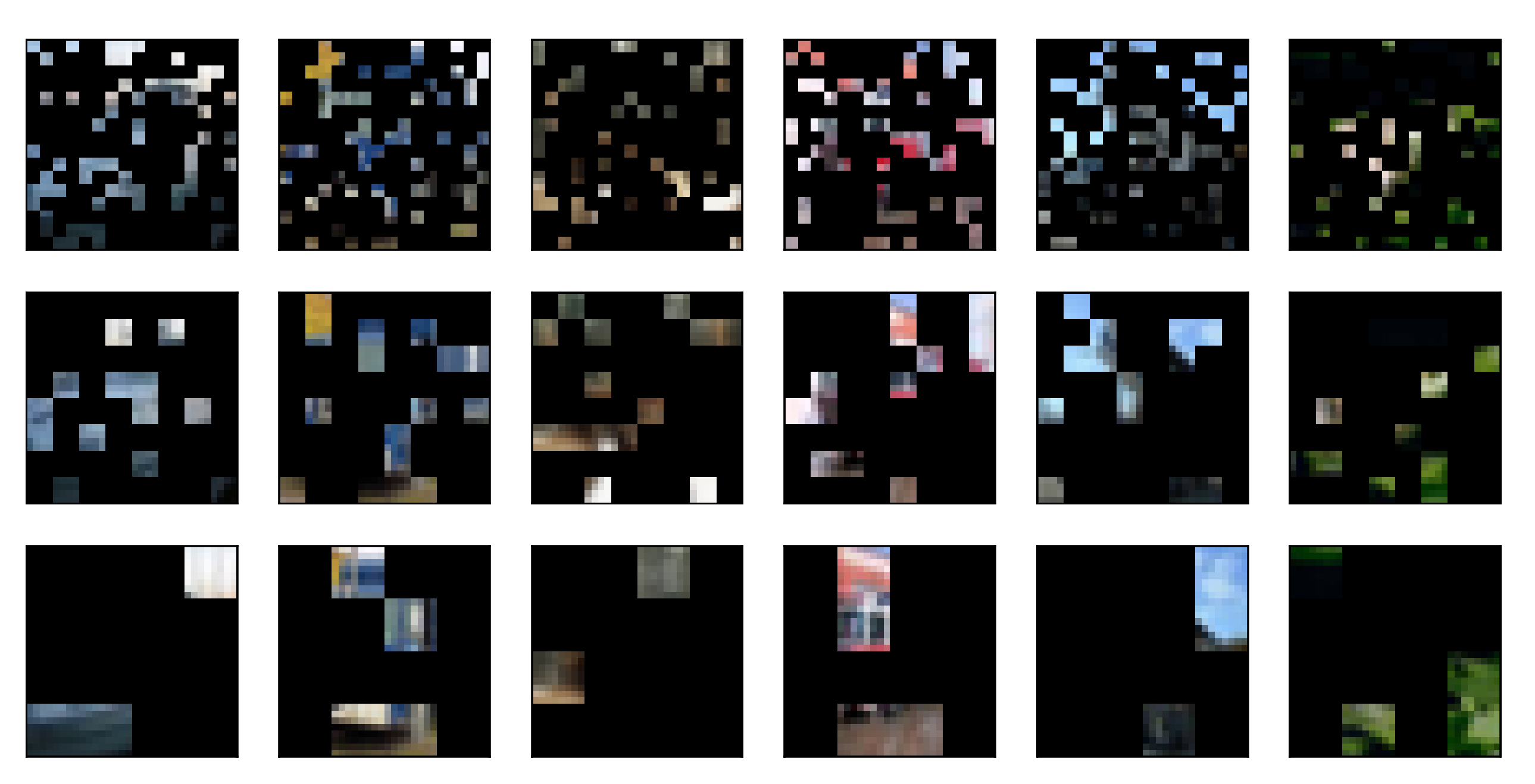
• Information density is often low in image data, as missing patches from an image can often be mostly recovered by a neural network structure [11] or by a human brain (as you can often reconstruct the missing parts of an object while looking at it through a fence).
• Adversarial attacks usually introduce a minor perturbation to inputs, which is likely to be reduced or cancelled by (randomly) covering part of the image.

Define $\tau :{\mathbb{R}}^d\times C\to {\mathbb{R}}^d$ as a masking operator, where C is a predefined set which has its cardinality depend on the number of grids that cover the input. For example, masking a $32\times 32$ image by using $8\times 8$ grids gives $2^{16}=65536$ possible ways of masking (2 possibilities for each grid, i.e., to apply masking or not to apply masking. The image is divided into $(32/8)\times (32/8)=16$ grids), so that in this case one may set $\left|C\right|=2^{64}$. An extreme case is that all grids are masked, but this can hardly happen as we pick up grids probabilistically. Suppose the original classifier $f_{\theta }$ is trained with sample set Z, and we use the sample set $Z\times C$ to retrain the existing structure into a new DNN model $f_{{\theta }^{\prime }}:{\mathbb{R}}^d\to \mathcal{Y}$ that is used to “simulate” the performance of $f_{\theta }$, in the sense that given $x\in \mathcal{X}$, so as to enhance the robustness of the model. At the same time, the attacker needs to generate effective adversarial noise for each image in $\left|C\right|$, which increases the difficulty of the attack and reduces the effect of the attack.

Compared with other adversarial defense methods, MAD does not need an additional denoising structure, or any change to the existing DNN, but still achieves state-of-the-art performance for adversarial defense against a wide variety of attack methods. Furthermore, because the attack algorithms are allowed to have access to the parameters of MAD, our defense seems to provide a way to withstand gray-box attacks, as the randomized masking technique may enforce attackers to consider an attack space of size exponential in the number of grids required to cover the input.

The random mask operation may occasionally cover the target in the image, especially when the target is small. Therefore, in the test phase, it is necessary to repeatedly test an input with randomized masking applied, in order to improve the accuracy of classification. Through the backpropagation of gradient and the output of intermediate convolution layers, a saliency map [31,32] or class activation map [33,34] can be calculated, which describes the attention of the neural network to different parts of the image. For adversarial samples, these highly activated parts may have a negative impact on the classification results of the neural network and can be eliminated by the mask operation. By combining additional information such as saliency map and class activation map, we plan to study how to mask images more effectively in our future work. In addition, we have to point out that it is in general difficult to represent the deep neural network by using a formal approach [35,36,37]. Therefore, in this paper, we mainly prove the effectiveness of the proposed method through experiments, and leave its formal proof as another future work.

References

1. Report. Neural Network Market to Reach $38.71 Billion, Globally, by 2023, Says Allied Market Research. 2020. Available online: https://www.globenewswire.com/fr/news-release/2020/04/02/2010880/0/en/Neural-Network-Market-to-reach-38-71-billion-Globally-by-2023-Says-Allied-Market-Research.html (accessed on 1 December 2022).
2. Szegedy, C.; Zaremba, W.; Sutskever, I.; Bruna, J.; Erhan, D.; Goodfellow, I.; Fergus, R. Intriguing properties of neural networks. In Proceedings of the ICLR, Banff, AB, Canada, 14–16 April 2014. [Google Scholar]
3. Goodfellow, I.J.; Shlens, J.; Szegedy, C. Explaining and harnessing adversarial examples. In Proceedings of the ICLR, San Diego, CA, USA, 7–9 May 2015. [Google Scholar]
4. Papernot, N.; McDaniel, P.; Jha, S.; Fredrikson, M.; Celik, Z.B.; Swami, A. The Limitations of Deep Learning in Adversarial Settings. In Proceedings of the 2016 IEEE European Symposium on Security and Privacy (EuroS&P), Saarbruecken, Germany, 21–24 March 2016; pp. 372–387. [Google Scholar] [CrossRef] [Green Version]
5. Ma, X.; Li, B.; Wang, Y.; Erfani, M.S.; Wijewickrema, N.R.S.; Houle, E.M.; Schoenebeck, G.; Song, D.; Bailey, J. Characterizing Adversarial Subspaces Using Local Intrinsic Dimensionality. In Proceedings of the ICLR, Vancouver, BC, Canada, 30 April–3 May 2018. [Google Scholar]
6. Cohen, G.; Sapiro, G.; Giryes, R. Detecting Adversarial Samples Using Influence Functions and Nearest Neighbors. In Proceedings of the 2020 IEEE/CVF Conference on Computer Vision and Pattern Recognition (CVPR), Seattle, WA, USA, 15–19 June 2020; pp. 14441–14450. [Google Scholar] [CrossRef]
7. Xu, W.; Evans, D.; Qi, Y. Feature Squeezing: Detecting Adversarial Examples in Deep Neural Networks. In Proceedings of the NDSS, San Diego, CA, USA, 18–21 February 2018. [Google Scholar]
8. Meng, D.; Chen, H. MagNet: A Two-Pronged Defense against Adversarial Examples. In Proceedings of the 2017 ACM SIGSAC Conference on Computer and Communications Security Association for Computing Machinery (CCS ’17), New York, NY, USA, 30 October–3 November 2017; pp. 135–147. [Google Scholar] [CrossRef]
9. Madry, A.; Makelov, A.; Schmidt, L.; Tsipras, D.; Vladu, A. Towards Deep Learning Models Resistant to Adversarial Attacks. In Proceedings of the ICLR, Vancouver, BC, Canada, 30 April–3 May 2018. [Google Scholar]
10. Mustafa, A.; Khan, S.; Hayat, M.; Goecke, R.; Shen, J.; Shao, L. Adversarial defense by restricting the hidden space of deep neural networks. In Proceedings of the ICCV, Seoul, Korea, 27 October–2 November 2019; pp. 3385–3394. [Google Scholar]
11. He, K.; Chen, X.; Xie, S.; Li, Y.; Dollár, P.; Girshick, R. Masked Autoencoders Are Scalable Vision Learners. In Proceedings of the 2022 IEEE/CVF Conference on Computer Vision and Pattern Recognition (CVPR), New Orleans, LA, USA, 21–23 June 2022; pp. 15979–15988. [Google Scholar] [CrossRef]
12. Papernot, N.; McDaniel, P.; Wu, X.; Jha, S.; Swami, A. Distillation as a Defense to Adversarial Perturbations Against Deep Neural Networks. In Proceedings of the 2016 IEEE Symposium on Security and Privacy (SP), San Jose, CA, USA, 22–26 May 2016; pp. 582–597. [Google Scholar] [CrossRef] [Green Version]
13. Kurakin, A.; Goodfellow, I.; Bengio, S. Adversarial examples in the physical world. In Proceedings of the ICLR Workshop, Toulon, France, 24–26 April 2017. [Google Scholar]
14. Liao, F.; Liang, M.; Dong, Y.; Pang, T.; Hu, X.; Zhu, J. Defense Against Adversarial Attacks Using High-Level Representation Guided Denoiser. In Proceedings of the 2018 IEEE/CVF Conference on Computer Vision and Pattern Recognition, Salt Lake City, UT, USA, 18–23 June 2018; pp. 1778–1787. [Google Scholar] [CrossRef] [Green Version]
15. Samangouei, P.; Kabkab, M.; Chellappa, R. Defense-GAN: Protecting classifiers against adversarial attacks using generative models. arXiv 2018, arXiv:1805.06605. [Google Scholar]
16. Salman, H.; Sun, M.; Yang, G.; Kapoor, A.; Kolter, J.Z. Denoised Smoothing: A Provable Defense for Pretrained Classifiers. In Proceedings of the NeurIPS 2020, Virtual, 6–12 December 2020. [Google Scholar]
17. Song, Y.; Kim, T.; Nowozin, S.; Ermon, S.; Kushman, N. PixelDefend: Leveraging Generative Models to Understand and Defend against Adversarial Examples. In Proceedings of the ICLR, Vancouver, BC, Canada, 30 April–3 May 2018. [Google Scholar]
18. Lee, S.; Lee, H.; Yoon, S. Adversarial Vertex Mixup: Toward Better Adversarially Robust Generalization. In Proceedings of the 2020 IEEE/CVF Conference on Computer Vision and Pattern Recognition (CVPR), Seattle, WA, USA, 13–19 June 2020; pp. 269–278. [Google Scholar] [CrossRef]
19. Potdevin, Y.; Nowotka, D.; Ganesh, V. An Empirical Investigation of Randomized Defenses against Adversarial Attacks. arXiv 2019, arXiv:1909.05580v1. [Google Scholar]
20. Gu, S.; Rigazio, L. Towards Deep Neural Network Architectures Robust to Adversarial Examples. In Proceedings of the ICLR Workshop, San Diego, CA, USA, 7–9 May 2015. [Google Scholar]
21. Cisse, M.; Bojanowski, P.; Grave, E.; Dauphin, Y.; Usunier, N. Parseval Networks: Improving Robustness to Adversarial Examples. In Proceedings of the 34th International Conference on Machine Learning ICML’17, Sydney, Australia, 6–11 August 2017; pp. 854–863. [Google Scholar]
22. Zoph, B.; Le, Q.V. Neural architecture search with reinforcement learning. arXiv 2016, arXiv:1611.01578. [Google Scholar]
23. Krizhevsky, A.; Hinton, G. Learning Multiple Layers of Features from Tiny Images; University of Toronto: Toronto, ON, Canada, 2009. [Google Scholar]
24. Netzer, Y.; Wang, T.; Coates, A.; Bissacco, A.; Wu, B.; Ng, A. Reading Digits in Natural Images with Unsupervised Feature Learning. In Proceedings of the NIPS Workshop on Deep Learning and Unsupervised Feature Learning, Sierra Nevada, Spain, 16–17 December 2011. [Google Scholar]
25. Lecun, Y.; Bottou, L.; Bengio, Y.; Haffner, P. Gradient-based learning applied to document recognition. Proc. IEEE 1998, 86, 2278–2324. [Google Scholar] [CrossRef] [Green Version]
26. Simonyan, K.; Zisserman, A. Very Deep Convolutional Networks for Large-Scale Image Recognition. In Proceedings of the ICLR, San Diego, CA, USA, 7–9 May 2015. [Google Scholar]
27. He, K.; Zhang, X.; Ren, S.; Sun, J. Deep Residual Learning for Image Recognition. In Proceedings of the 2016 IEEE Conference on Computer Vision and Pattern Recognition (CVPR), Las Vegas, NV, USA, 27–30 June 2016; pp. 770–778. [Google Scholar] [CrossRef] [Green Version]
28. Rauber, J.; Brendel, W.; Bethge, M. Foolbox: A Python toolbox to benchmark the robustness of machine learning models. In Proceedings of the Reliable Machine Learning in the Wild Workshop, 34th International Conference on Machine Learning, Sydney, Australia, 6–11 August 2017. [Google Scholar]
29. Carlini, N.; Wagner, D. Towards Evaluating the Robustness of Neural Networks. In Proceedings of the 2017 IEEE Symposium on Security and Privacy (SP), San Jose, CA, USA, 22–29 May 2017; pp. 39–57. [Google Scholar] [CrossRef]
30. Levine, A.; Feizi, S. Robustness certificates for sparse adversarial attacks by randomized ablation. In Proceedings of the AAAI Conference on Artificial Intelligence, New York, NY, USA, 7–12 February 2020; Volume 34, pp. 4585–4593. [Google Scholar]
31. Simonyan, K.; Vedaldi, A.; Zisserman, A. Deep inside convolutional networks: Visualising image classification models and saliency maps. arXiv 2013, arXiv:1312.6034. [Google Scholar]
32. Cheng, L.; Fang, P.; Liang, Y.; Zhang, L.; Shen, C.; Wang, H. TSGB: Target-Selective Gradient Backprop for Probing CNN Visual Saliency. IEEE Trans. Image Process. 2022, 31, 2529–2540. [Google Scholar] [CrossRef] [PubMed]
33. Zhou, B.; Khosla, A.; Lapedriza, A.; Oliva, A.; Torralba, A. Learning Deep Features for Discriminative Localization. In Proceedings of the 2016 IEEE Conference on Computer Vision and Pattern Recognition (CVPR), Las Vegas, NV, USA, 27–30 June 2016; pp. 2921–2929. [Google Scholar] [CrossRef] [Green Version]
34. Chattopadhay, A.; Sarkar, A.; Howlader, P.; Balasubramanian, V.N. Grad-CAM++: Generalized Gradient-Based Visual Explanations for Deep Convolutional Networks. In Proceedings of the 2018 IEEE Winter Conference on Applications of Computer Vision (WACV), Lake Tahoe, NV, USA, 12–15 March 2018; pp. 839–847. [Google Scholar] [CrossRef] [Green Version]
35. Seshia, S.A.; Desai, A.; Dreossi, T.; Fremont, D.J.; Ghosh, S.; Kim, E.; Shivakumar, S.; Vazquez-Chanlatte, M.; Yue, X. Formal Specification for Deep Neural Networks. In Proceedings of the Automated Technology for Verification and Analysis; Lahiri, S.K., Wang, C., Eds.; Springer: Berlin/Heidelberg, Germany, 2018; pp. 20–34. [Google Scholar] [CrossRef]
36. Li, Y.; Yuan, Y. Convergence analysis of two-layer neural networks with relu activation. arXiv 2017, arXiv:1705.09886v2. [Google Scholar]
37. Seshia, S.A.; Sadigh, D.; Sastry, S.S. Toward Verified Artificial Intelligence. Commun. ACM 2022, 65, 46–55. [Google Scholar] [CrossRef]
Figure 1. An overview of the MAD scheme.
Algorithms 15 00461 g001
Figure 2. The red line shows the relationship between test accuracy and number of repetitions for 3 / 4 masked images from CIFAR-10, and the green line shows the amount of time (in seconds) that is required to test 10,000 images.
Algorithms 15 00461 g002
Figure 3. An experiment showing weakened effect of partially removed adversarial vectors generated from CIFAR-10 samples on the accuracy of a VGG16 network.
Algorithms 15 00461 g003
Figure 4. Images from CIFAR-10 with different masking rates applied. From top to bottom, 1 / 3 , 1 / 2 , and 3 / 4 rates are respectively applied on the same images.
Algorithms 15 00461 g004
Figure 5. The 3 / 4 masked images from CIFAR-10 with different grid sizes: from top to bottom, 2 × 2 , 4 × 4 and 8 × 8 grids are used for masking the same images.
Algorithms 15 00461 g005