Batch Acquisition for Parallel Bayesian Optimization—Application to Hydro-Energy Storage Systems Scheduling ^†

Abstract

Bayesian Optimization (BO) with Gaussian process regression is a popular framework for the optimization of time-consuming cost functions. However, the joint exploitation of BO and parallel processing capabilities remains challenging, despite intense research efforts over the last decade. In particular, the choice of a suitable batch-acquisition process, responsible for selecting promising candidate solutions for batch-parallel evaluation, is crucial. Even though some general recommendations can be found in the literature, many of its hyperparameters remain problem-specific. Moreover, the limitations of existing approaches in terms of scalability, especially for moderately expensive objective functions, are barely discussed. This work investigates five parallel BO algorithms based on different batch-acquisition processes, applied to the optimal scheduling of Underground Pumped Hydro-Energy Storage stations and classical benchmark functions. Efficient management of such energy-storage units requires parallel BO algorithms able to find solutions in a very restricted time to comply with the responsive energy markets. Our experimental results show that for the considered methods, a batch of four candidates is a good trade-off between execution speed and relevance of the candidates. Analysis of each method’s strengths and weaknesses indicates possible future research directions.

1. Introduction

Integrating renewable energy resources is a key challenge to ensure the transition towards a low-carbon energy system. Electricity storage systems provide a valuable solution to compensate for the uncertain production, thus offering sustainable means to increase the flexibility of the system [1]. An appropriate option regarding storage technologies is offered by Underground Pumped Hydro-Energy Storage (UPHES). However, in modern competitive energy networks, individual actors rely on efficient operational strategies, enabling them to hedge the uncertainty of renewable energy resources. It is thus essential to dispose of efficient tools to make informed and fast decisions at the different time steps of the energy markets (e.g., from long-term towards real-time) [2]. From the operator’s point of view, the quality of a decision is measured as a profit, so let us assume that for a decision $\mathit{x}\in {\mathbb{R}}^d$, the expected profit of a UPHES operator is given by $f:{\mathbb{R}}^d\to \mathbb{R};\mathit{x}\mapsto y=f\left(\mathit{x}\right)$. The simulator, f, is then considered as a time-consuming Black-Box function, which is further described in Section 2.1.

The complexity of physical phenomena in UPHES devices usually calls for model-based approximations [3]. Using these approximations, evaluation of the expected profit is fast and classical optimization methods (e.g., dynamic programming, genetic algorithms) can be applied to optimize the UPHES scheduling within a reasonable time budget [4,5]. However, approximations may lead to unreliable simulations, motivating the recent proposal of a more robust model-based UPHES simulator in Toubeau et al.[3]. This comes at a much higher simulation cost compared to conventional model-based approximations.

With this increased simulation cost, existing optimization approaches become impractical, as operational constraints require scheduling optimization to be completed within approximately 30 min. This motivates us to investigate the use of surrogate models to (partially) replace the time-consuming simulator, in conjunction with parallel evaluations of the expected profit. To the best of our knowledge, surrogate-based optimization has never been applied to the UPHES scheduling problem. In our previous work [2], we demonstrated that Bayesian Optimization (BO) can be handy in management problems in electrical engineering.

More precisely, Parallel BO (PBO) is emerging as a powerful framework for such problems. This surrogate-guided optimization approach relies on a surrogate model—often Gaussian Process (GP) regression. Based on that model, an Acquisition Function (AF) is defined to assess the value of any candidate point. Optimizing the AF yields the best candidate point according to this specific AF. In this way, only valuable (still in the sense of the AF) points are evaluated in parallel using the time-consuming simulator. Consequently, the overall optimization time can be considerably reduced. This is essential due to the time constraint arising from both the organization of energy markets and the complex modeling of physical and economic constraints of pumped-hydro systems.

More generally speaking, we refer to the process responsible for selecting the next candidate points as the Acquisition Process (AP). Clearly, the choice of the AP is of crucial importance to balance the exploration and exploitation during the optimization process. However, only a few general recommendations can be extracted from the literature, especially considering the batch querying AP which is usually problem-dependent. In addition, the main potential for exploiting parallel computing lies in the batch-parallel evaluation of the candidates. Therefore, the AP must be able to provide a batch of valuable candidates. Various approaches are presented in Shahriari et al. [6], however, batch selection remains a challenging question, especially for large batch sizes and small amounts of time. Indeed, the computational overhead of surrogate-related algorithm components is rarely considered and usually judged as negligible with respect to simulation time [7]. Furthermore, the efficiency of large batches of candidates is often lesser than that of the same number of candidates taken sequentially [8].

In this paper, we investigate several parallel batch-based algorithms using different APs, and we compare the optimized average profit: q-Efficient Global Optimization with Kriging Believer (KB) heuristic (KB-q-EGO) from Ginsbourger, Le Riche and Carraro [9] (2008) and a revisited version allowing multi-infill criteria sampling (mic-q-EGO) inspired by Liu et al. [10] and Wang et al. [11]; Monte Carlo-based q-EGO (MC-based q-EGO) from Balandat et al. [12] (2020); Binary Space Partitioning EGO (BSP-EGO) from Gobert et al. [13] (2020); and TrUst Region BO (TuRBO) from Eriksson et al. [14] (2019). Experiments are conducted with different batch sizes to evaluate and compare the scalability of the approaches. A thorough investigation of the different approaches is required to identify the most suitable algorithm that responds to the specificities of the UPHES optimization problem. Indeed, the optimization must be conducted in a restricted time and, contrary to common assumption, the acquisition time is not negligible compared to the simulation time. Consequently, the acquisition time needs to be taken into account in order to perform an efficient optimization. Hence, the main contribution of this paper is the comparison of several PBO approaches in view of their application to a current concern in energy production.

The conducted study reveals that all investigated BO algorithms have poor scalability regarding parallel efficiency. Indeed, increasing the batch sizes obviously comes with the management of a larger data set. Consequently, a decrease in the number of performed cycles in a restricted time is expected, since the sequential part grows larger. Ideally, for an equivalent number of simulations, whatever the batch size, the final outcomes would be comparable. However, and despite the potentially larger number of simulations gained by parallelization, the final outcome of the algorithms is often worse with high batch sizes (8 or 16 compared to 2 or 4) within a fixed time budget.

In Section 2.1, a detailed explanation of the complex UPHES operation is provided along with a mathematical formulation of the resulting optimization problem. In Section 2.2, the PBO algorithms designed to optimize UPHES station management are presented with a focus on their specificities. Section 3 is dedicated to experiments and results, where the outcomes from different algorithms are compared. In Section 4, we discuss the experimental results. Finally, conclusions are drawn in Section 5 and we outline possible future research directions to overcome the observed limitations of PBO.

2. Material and Methods

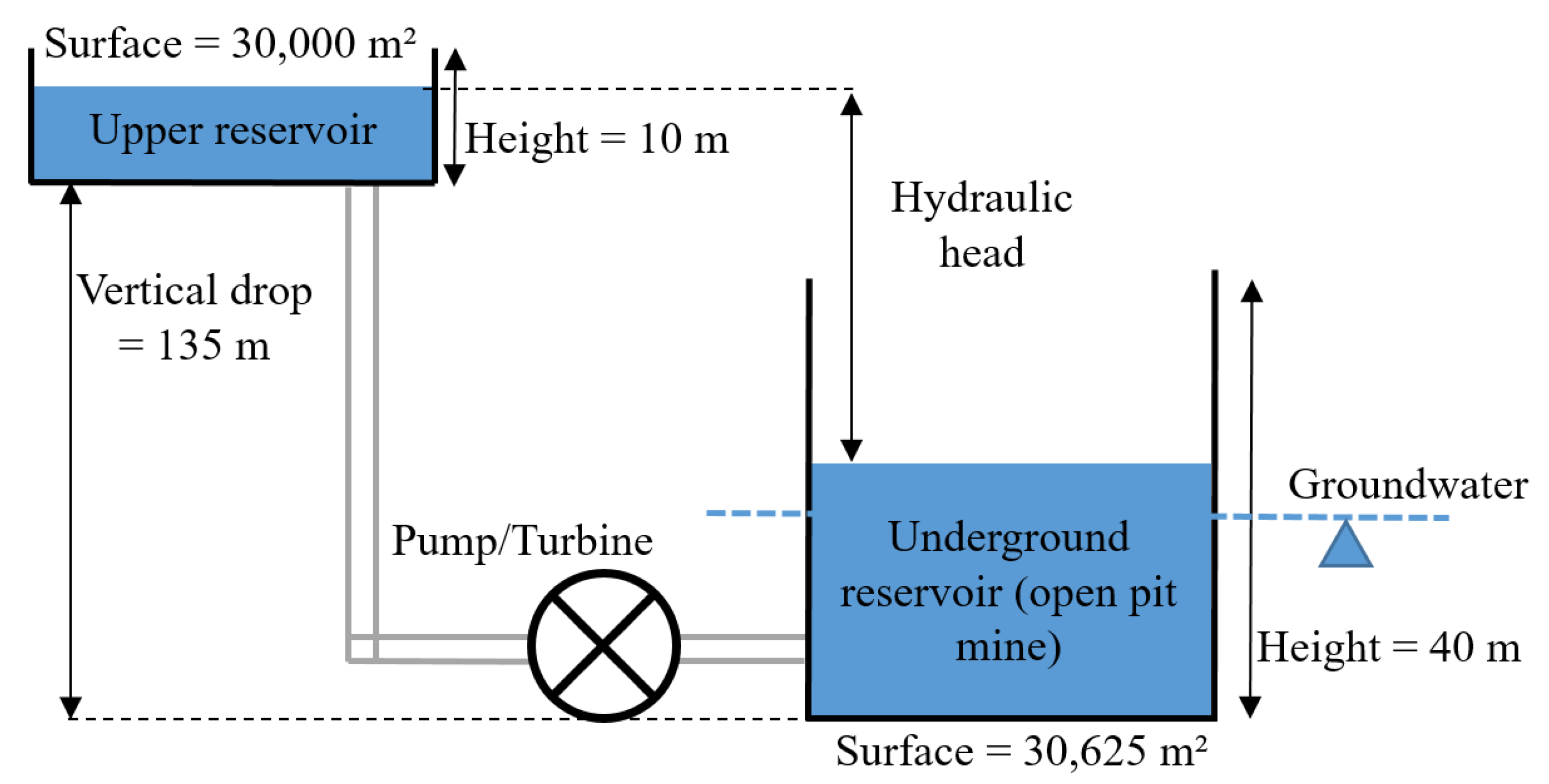
2.1. Underground Pumped Hydro-Energy Storage

Due to their ability to quickly and cost-effectively mitigate energy imbalances, Pumped Hydro-Energy Storage (PHES) stations offer an appropriate storage solution. PHES plants are composed of (at least) a lower and an upper reservoir from which water is exchanged to either produce or store energy. In off-peak periods, production might exceed consumption such that energy is saved by pumping water from the lower basin into the upper one. It then provides a substantial reserve of energy that can be later released when needed, e.g., to maintain the transmission grid stability. Recent progress in power electronics has enabled PHES units to operate with a reliable variable-speed feature in both pump and turbine modes. The flexibility offered by these facilities is highly valuable. Indeed, it improves the economic efficiency of existing resources such as wind farms or thermal power plants [15,16], and provides ancillary services to ensure grid stability (such as frequency control or congestion management).

The inherent potential of PHES units leads to the development of new technological solutions such as Underground PHES (UPHES) for which the lower basin is located underground. A significant advantage of UPHES is the limitation of expenses from civil engineering works thanks to the recycling of end-of-life mines or quarries. These stations have a very limited impact on the landscape, vegetation and wildlife, and are not limited by topography so that more sites can be exploited [17]. In the current competitive framework governing the electricity sector, UPHES units are exploited with the objective of return on investment. Consequently, the profit of such stations must be maximized. This task is challenging since the UPHES operation is governed by two main nonlinear effects that cannot be easily modeled with traditional analytical models [3].

Firstly, groundwater exchanges between the reservoirs and their hydro-geological porous surroundings may occur. This situation typically arises for UPHES when the waterproofing work is not feasible or uneconomical [18]. Secondly, UPHES units are generally subject to important variations of the net hydraulic head (i.e., the height difference between water levels in the reservoirs). These variations are referred to as the head effects [19], and are typically quantified through laboratory measurements on a scaled model of the hydraulic machines [20]. This characterization of head effects is important since the head value defines both the safe UPHES operating range as well as the efficiency of both pump and turbine processes. In this way, the safe operating limits in pump and turbine modes continuously vary over time with regard to head variations. In general, the performance curves of UPHES stations are difficult to model since they present a non-convex and non-concave behavior.

Directly integrating these effects into model-based optimization (which maximizes the UPHES profit in the different market floors) implies a high computational burden or strong assumptions that may jeopardize the feasibility of the obtained solution. To address these issues, a simulation-based BO strategy has been developed in this work. The simulator, which is a black box from the user perspective (developed independently without access to the source code), returns the daily UPHES profit accounting for all techno-economic constraints. The full description of physical and economical constraints can be found in Toubeau et al. [21].

This simulator is denoted as f in the following and, according to a decision vector $\mathit{x}\in {\mathbb{R}}^{12}$, it returns the expected profit $y=f\left(\mathit{x}\right)\in \mathbb{R}$. The 12-dimensional decision vector includes 8 decision variables to participate in the different time slots of the energy market, and 4 to the reserve market (i.e., provision of ancillary services). The number of decision variables is set in accordance with standard recommendations of electrical engineering. It is subject to modification in order to gain more flexibility in future studies. The objective is then to find the decisions that maximize the daily expected profit:

$${\mathit{x}}_{opt}={argmax}_{\mathit{x}\in \Omega }f\left(\mathit{x}\right),$$

where $\Omega$ is the domain (or design space). The objective function f also involves the constraints and deals with them by adding a penalty term inside the simulator.

These UPHES decisions must comply with hydraulic and electro-mechanical constraints over the whole daily horizon. This results in a challenging optimization problem (embedded in the simulator), which is discontinuous (from the cavitation effects of the pump-turbine machine that incur unsafe operating zones), nonlinear (from the complex performance curves of the unit), mixed-integer (to differentiate the pump-turbine-idle operation modes), which is subject to uncertainties (e.g., on water inflows and market conditions). The formulation used in this paper can be found in [21].

With full model-based optimization, errors caused by the inherent modeling approximations (typically, linearizations), required to ensure computational tractability of complex effects (i.e., nonlinear water levels within reservoirs, penstock head loss and head-dependent pump/turbine performance curves) may lead to infeasible solutions [3]. Relying instead on surrogate models may provide an efficient and robust solution to this problem. According to the two surveys of Taktak and D’Ambrosio [4], and Steeger, Barroso, and Rebennack [5], this kind of management problem in electrical engineering is typically solved using Mixed-Integer (Linear) Programming [22], dynamic programming [23] or nonlinear programming [24]. Current techniques also involve meta-heuristics such as Genetic Algorithm  [25] or Particle Swarm Optimization [26]. However, we are not aware of any BO or surrogate-based optimization approaches for the UPHES management problem.

Since the simulator is time-consuming (such that we cannot perform a large number of simulations during the available time), a judicious choice is to resort to PBO to find a good decision vector. Indeed, a decision must in practice be taken within tens of minutes at most. In this context of a very limited time budget and numerical simulations lasting 10 s on average, parallel computing offers an efficient tool to improve the search within a fixed wall time. In particular, as it usually provides good candidate solutions with a small number of evaluations and short time, PBO appears to be a natural choice. Usually, BO assumes that the time-cost associated with the model fitting and the AP is negligible compared to evaluation time. However, in the UPHES optimization problem, the simulator is considered costly because the optimization budget is defined as a time period. In this context, model fitting and AP cannot be neglected.

2.2. Parallel Bayesian Optimization

The concept has been introduced by Kushner [27] and later developed by Mockus et al. [28] before being popularized by Jones et al. [29]. The general idea of BO is to fit a probabilistic predictive model of the black-box objective function f—the simulator—in order to guide the optimization process. Indeed, f being time-consuming, we cannot afford to query a large number of simulations. Therefore, the surrogate model is used to evaluate the utility of a candidate point before it is evaluated with the costly simulator. This utility measure is often called AF, but also Infill Criteria (IC) or figure of merit. It uses the predicted value of the surrogate as well as the prediction variance provided by probabilistic models such as Gaussian Processes (GP). One famous example of AF is the Expected Improvement (EI) used in Efficient Global Optimization (EGO) [29]. BO operates in a loop composed of (i) fitting a metamodel, (ii) searching for the most valuable candidate(s) to simulate, (iii) simulation of the candidate(s). The three steps are referred to as a cycle.

BO involves two key elements: the definition of a surrogate model $\mathcal{M}$ that provides a prediction ${\widehat{y}}_{cand}$ for any candidate point ${\mathit{x}}_{cand}$ as well as a measure of uncertainty $\sigma \left({\mathit{x}}_{cand}\right)$, and an AP that proposes a (batch of) valuable point(s) for evaluation.

Many AFs have been proposed over the past decades. Shahriari et al. [6] propose a classification of the different AFs: (i) optimistic strategy—using best case scenario regarding the uncertainty such as Gaussian Process Upper Confidence Bound [30]; (ii) Improvement Based—using the improvement defined as $I\left(\mathit{x}\right)=max(f_{min}-f\left(\mathit{x}\right),0)$, such as Probability of Improvement [27], Expected Improvement [29,31] (EI), Scaled EI [32]; and Information Based strategy—focusing on the information rather than the improvement, such as Thompson Sampling, Entropy Search [33], Predictive Entropy Search [34] or Max-Value Entropy Search [35].

Exploiting parallel computing requires being able to provide a batch of candidate points for batch parallel evaluation. In addition to intrinsic multi-point criteria such as q-EI, various strategies are adopted to achieve this goal. One may choose to rely on a single point criterion either using it several times [13,36], or trying to localize distinct local optimal values of the AFs [37,38]. It is also possible to rely on multiple single points criteria hoping that they yield distinct candidates [11,39] or even optimize them in a multi-objective way to find a compromise between ICs [40,41]. Five different APs are investigated in this paper and presented in the following.

2.2.1. Gaussian Process Regression

Usually, a GP surrogate model is used. The latter assumes a linear relation between inputs $\mathit{x}$ and outputs y, such that $y={\omega }^T\mathit{x}+ϵ$. The observation/output is often considered noisy, hence the $ϵ$ error term, which is assumed Gaussian ($ϵ\sim \mathcal{N}(0,{\sigma }^2)$). As explained in [42], a Bayesian approach assumes a prior distribution over weights $\omega$, which is also Gaussian ($\omega \sim \mathcal{N}(0,\Sigma )$) and constitutes the prior belief. Starting from that belief, it is possible to update the prior distribution with knowledge of the data $(\mathit{X},\mathit{y})$, which is defined as the posterior distribution. Using the Bayes rule the posterior is expressed as

$$\mathrm{posterior}=\frac{\mathrm{likelihood}\times \mathrm{prior}}{\mathrm{evidence}}.$$

(1)

With previous notations, Equation (1) becomes

$$p\left(\omega |\mathit{X},\mathit{y}\right)=\frac{p\left(\mathit{y}|\mathit{X},\omega \right)p\left(\omega \right)}{p\left(\mathit{y}|\mathit{X}\right)}=\frac{p\left(\mathit{y}|\mathit{X},\omega \right)p\left(\omega \right)}{{\int }_{\omega }p\left(\mathbf{y}|\mathbf{X},\omega \right)p\left(\omega \right)d\omega }.$$

(2)

The evidence $p\left(y\right|\mathit{X})$ is also referred to as the normalizing constant and can be expressed as the marginal likelihood by marginalizing over the weights $\omega$. Often, input data $\mathit{X}$ are projected into a feature space using a set of basis functions $\Phi \left(\mathit{x}\right)={({\varphi }_1\left(\mathit{x}\right),\cdots ,{\varphi }_k\left(\mathit{x}\right))}^T$ which leads to the following model: $y={\omega }^T\Phi \left(\mathit{x}\right)+ϵ$. Denoting $\Phi =\Phi \left(\mathit{X}\right)$, we can simply replace $\mathit{X}$ by $\Phi$ in Equation (2). Knowing the distribution of the posterior $p\left(\omega |\Phi ,\mathit{y}\right)\sim \mathcal{N}\left(\frac{1}{{\sigma }^2}{A}^{-1}\Phi \mathit{y},A^{-1}\right)$ with $A={\sigma }^{-2}\Phi {\Phi }^T+{\Sigma }^{-1}$, it is possible to make inference. The predictive distribution of a design point ${\mathit{x}}^{*}$ writes

$$p\left(y^{*}|\Phi ,\mathit{y},{\mathit{x}}^{*}\right)={\int }_{\omega }p\left(y^{*}|\omega \right)p\left(\omega |\Phi ,\mathit{y}\right)d\omega \sim \mathcal{N}\left(\frac{1}{{\sigma }^2}{\Phi \left({\mathit{x}}^{*}\right)}^T{A}^{-1}\Phi \mathit{y},{\Phi \left({\mathit{x}}^{*}\right)}^T{A}^{-1}\Phi \left({\mathit{x}}^{*}\right)\right)$$

(3)

and is also Gaussian. It can be shown that Equation (3) can be equivalently written as:

$$p\left(y^{*}|\Phi ,\mathit{y},{\mathit{x}}^{*}\right)\sim \mathcal{N}\left(\Phi {\left({\mathit{x}}^{*}\right)}^T\Sigma \Phi {(K+{\sigma }^{2}I)}^{-1}\mathit{y},K^{**}-K^{*·}{(K+{\sigma }^{2}I)}^{-1}{K}^{·*}\right)$$

(4)

where $K={\Phi }^T\Sigma \Phi$ is known as the covariance matrix and $K^{\left(1\right)\left(2\right)}=\Phi {\left({\mathit{x}}^{\left(1\right)}\right)}^T\Sigma \Phi \left({\mathit{x}}^{\left(2\right)}\right)=k\left(x^{\left(1\right)},x^{\left(2\right)}\right)$. The k function is referred to as the covariance kernel and $K={\left(k({\mathit{x}}_i,{\mathit{x}}_j)\right)}_{i,j\in \{1,\dots ,n\}}$ and is chosen by the user among other hyperparameters. Following previous notation, we denote ${\left(k({\mathit{x}}^{*},{\mathit{x}}_j)\right)}_{j\in \{1,\dots ,n\}}=K^{*,·}={\left({\Phi }^{*}\right)}^T\Sigma \Phi$.

2.2.2. Acquisition Process for Optimization

The BO framework is illustrated in Algorithm 1. The mentioned parallel algorithms follow the same scheme but differ in the candidate selection phase which is represented by the optimization of the $\alpha$ function in Algorithm 1. Line 4 of Algorithm 1 states that the algorithm is searching for the best (batch of) candidate(s) in terms of $\alpha$ to be added. The candidate selection, referred to as the AP, is also an optimization problem sometimes called inner optimization.

Algorithm 1 Bayesian Optimization

1: Initial DoE: $\{\mathit{X},\mathit{y}\}$ 2: while Budget available do 3:     $\mathcal{M}=\mathcal{GP}\left(\right\{\mathit{X},\mathit{y}\left\}\right)$ 4:     ${\mathit{x}}_{new}=argma{x}_{\Omega }\left(\alpha \left(\mathit{x}\right)\right)$ 5:     $y_{new}=f\left({\mathit{x}}_{new}\right)$ 6:     $(\mathit{X},\mathit{y})=(\mathit{X},\mathit{y})\cup ({\mathit{x}}_{new},y_{new})$ 7: end while

Even though BO and GP seems a legitimate choice in the context of optimization with a relatively small budget and strong time constraint the choice of the AP is difficult and must be done in accordance with the time constraint. This is why several different APs presenting different behaviors are investigated in this study.

• The KB-q-EGO algorithm refers to the work of Ginsbourger et al. [9,36] where they present heuristics to approximate multi-point criteria which are difficult to exploit when the required number of candidates exceeds $q=2$ (q being the batch size, also denoted as $n_{batch}$ throughout this paper). The idea is to replace the time-consuming simulation with a fast-to-obtain temporary/fantasy value in order to update the surrogate model $\mathcal{M}$, which allows the suggestion of a new distinct candidate. In the KB heuristic, it is decided to trust the surrogate model (hence, Kriging Believer) and use its output as fantasy value. The operation can be repeated sequentially until q design points are selected. Then, it is possible to exactly evaluate them in parallel and replace the temporary values with the real costs. However, this strategy has the major drawback of requiring q sequential updates of $\mathcal{M}$ per cycle. In Ginsbourger et al. [9], inside the heuristic loop, the Kriging model is used without hyperparameter re-estimation. To preserve this aspect and in order to alleviate the fitting cost, the budget allocated to the intermediate fitting of the surrogate model is reduced compared to a full update performed at the beginning of a cycle.
• We propose Multi-infill-criteria q-EGO (mic-q-EGO), an alternative AP that uses multiple IC in the same cycle in order to limit the number of surrogate fitting operations. This approach is a variation of q-EGO using a multi-infill strategy such as in Liu et al. [10] or Wang et al. [11]. Using multiple AFs allows to select different candidate points without updating the surrogate model, assuming that their optimization yields distinct candidate points. Moreover, it has been observed that resorting to different AFs can favorably impact the objective value, especially when the batch size is large. Indeed, repeatedly updating $\mathcal{M}$ using non-simulated data may degrade the relevance of proposed candidates [8]. Since standard EI, used as the primary criterion, is known to sometimes over-explore the search space, it is decided to rely on the Upper Confidence Bound (UCB) criterion to improve the exploitation. In this paper, two ICs are used with the same number of candidates from each criterion. Therefore, albeit generalizable to more criteria not necessarily evenly distributed, the description of Algorithm 2 considers the previous statement for sake of simplicity. We denote ${\alpha }_1$ and ${\alpha }_2$ the two AFs, then for the same model, a candidate can be chosen according to each AF (line 6 and 7). Despite not being implemented yet, the optimizations of ${\alpha }_{1,2}$ could be conducted in parallel. If more candidates are required, a partial model update is necessary (line 11) using the predicted value ($y_{PV}$) as suggested in the KB heuristic. The loop continues until q candidate points are selected.
• BSP-EGO [13] is an algorithm developed by the authors with the objective of tackling time-consuming black-box objective functions for which the execution time does not dominate the acquisition time. It uses a dynamic binary partition of the search space to optimize the AF inside sub-regions. Thereby, a local AP based on a global model is conducted simultaneously in each sub-domain. Candidate points coming from sub-regions are aggregated and sorted according to their infill value in order to choose the $n_{batch}$ most promising ones. By the end of a cycle, the partition evolves in accordance with the performance of each sub-region: the one containing the best candidate in terms of the AF will be split further while the supposedly less valuable sub-regions are merged. At any time, the partition covers the entire search space and involves the same number of sub-regions. The number of sub-regions is chosen to be a multiple of $n_{batch}$ to balance the load between parallel workers. Having $n_{cand}>n_{batch}$ avoids sampling into clearly low potential sub-regions by letting the choice of $n_{batch}$ among $n_{cand}$. Typically in this work, $n_{cand}=2\times n_{batch}$. As the supposed best sub-region is split at each cycle, diversification is imposed at the beginning, while intensification is favored as the budget fades. This considerably reduces the acquisition time compared to q-EGO since it can be conducted in parallel thanks to the spatial decomposition, which is valuable since the optimization must be completed in very restricted time.
• MC-based q-EGO from the BOTorch library, developed by Balandat et al. [12] uses the reparameterization trick from Wilson et al. [43] and (quasi) MC sampling for estimation of multi-points AF - EI in this study. The latter allows to approximate the AF value and time-efficiently optimize the batch of candidates. However, optimizing the multi-points AF still requires optimizing a $n_{batch}\times d$ objective function which can become tricky and, depending on the inner optimization algorithm, time-consuming when increasing $n_{batch}$.
• TuRBO [14] uses trust regions to progressively reduce the size of the search space with the objective of compensating for the overemphasized exploration resulting from global AP. The trust region takes the form of a hyper-rectangle centered at the best solution found so far. The side length for each dimension of the hyper-rectangle is scaled according to the length scale ${\lambda }_i$ from the GP model while maintaining a total volume of $L^d$. Then, an AP is performed in the trust region that yields a batch of candidates. One or several trust regions can be maintained simultaneously. In this work, one trust region is used with multi-point EI (q-EI) evaluated through MC approximation, similarly to MC-based q-EGO. Therefore, the main characteristic of TuRBO is that the search space is re-scaled according to the length scale of the $\mathcal{GP}$ model and evolves according to the following rule: if the current cycle improves the best solution, the trust region is extended, or else it is shrunk. As mentioned in Eriksson et al., running with only one trust region including the whole domain $\Omega$, TuRBO is equivalent to running the standard q-EGO algorithm.

Algorithm 2 Multi-infill q-EGO acquisition process

1: $\mathcal{M}$: Surrogate model 2: $\Omega$: Search space 3: $ct=0$; initialize counter 4: ${\mathit{X}}_{batch}=\left\{\right\},{\mathit{y}}_{batch}=\left\{\right\}$ 5: while ct $<q$ do 6:     ${\mathit{x}}_{new\_1}=argma{x}_{\mathit{x}\in \Omega }{\alpha }_1\left(\mathcal{M},\mathit{x}\right)$ 7:     ${\mathit{x}}_{new\_2}=argma{x}_{\mathit{x}\in \Omega }{\alpha }_2\left(\mathcal{M},\mathit{x}\right)$ 8:     ${\mathit{X}}_{batch}={\mathit{X}}_{batch}\cup {\mathit{x}}_{new\_1}\cup {\mathit{x}}_{new\_2}$ 9:     ${\mathit{y}}_{batch}={\mathit{y}}_{batch}\cup y_{PV}\left({\mathit{x}}_{new\_1}\right)\cup y_{PV}\left({\mathit{x}}_{new\_2}\right)$ 10:     $ct\leftarrow ct+2$ 11:     $\mathcal{M}\leftarrow partial\_fit(\mathbf{X}\cup {\mathit{X}}_{batch},\mathit{y}\cup {\mathit{y}}_{batch})$ 12: end while 13: Returns ${\mathit{X}}_{batch}$ to exactly evaluate in parallel

Both KB-q-EGO and MC-based q-EGO algorithms are common parallel BO approaches that use a global model fitted on the entire data set. KB-q-EGO relies on a sequential heuristic to select a batch of candidates while MC-based q-EGO uses Monte Carlo sampling to evaluate the q-points AF and create batches of candidates. The main difference is that MC-based q-EGO considers the combined utility of the set of candidates while KB-q-EGO only considers one candidate at a time, sequentially. mic-q-EGO uses a global model and exploits different AFs to limit the number of surrogate updates and add a diversity in candidates. BSP-EGO also uses a global model but uses spatial decomposition in order to perform independent parallel APs and reduce the acquisition time compared to the sequential heuristic of q-EGO and KB-q-EGO algorithms. Both mic-q-EGO and BSP-EGO use a single point AF multiple times, as in the standard KB-q-EGO algorithm. As MC-based q-EGO TuRBO operates with a multi-points AF evaluated with MC approximation. However, the latter is optimized on trust region(s) so that AP(s) are locally performed to provide a batch of candidates. In this study, TuRBO only uses one trust region, as presented in the BOTorch framework [12]. It then operates as MC-based q-EGO inside a trust region. A notable difference between all algorithms lies in the way they exploit parallelism: KB-q-EGO, mic-q-EGO MC-based q-EGO and TuRBO algorithms only use batch parallelization for the evaluation of the candidates, while BSP-EGO also parallelizes the AP.

2.3. Problem Instances

2.3.1. UPHES Management

The experimental evaluation uses a real-world UPHES station located in Maizeret (Belgium) as a test case. Its configuration is shown in Figure 1. The lower basin is a former underground open pit mine subject to groundwater exchanges. Furthermore, the surface of both reservoirs is relatively limited, which results in significant head effects. The specific features of the UPHES unit are taken into account in the simulator implemented in the Resource-Action-Operation language [44] and Matlab. The UPHES nominal output ranges (for the nominal value of the hydraulic head) are respectively [6, 8] MW and [4, 8] MW in pump and turbine modes and the energy capacity is 80 MWh. The optimization problem involves 12 decision variables.

2.3.2. Benchmark Functions

Three classical benchmark functions are used to validate the approaches: Rosenbrock, Ackley and Schwefel functions [45]. The three functions are optimized with 12 decision variables to remain consistent with the UPHES problem. We consider the minimization of previous functions defined on search spaces presented in

Table 1. Definition of the benchmark functions.

Name	Expression	$\mathit{\Omega }$	${\mathit{f}}_{\mathbf{min}}$
Rosenbrock	${\displaystyle \sum _{i=1}^{11}}100{(x_i^2-x_{i+1})}^2+{(x_i-1)}^2$	${\left[-5;10\right]}^{12}$	0
Ackley	$-20exp(-0.2\sqrt{\frac{1}{12}{\displaystyle \sum _{i=1}^{12}}{x}_i^2})-exp\left(\frac{1}{12}{\displaystyle \sum _{i=1}^{12}}cos\left(2\pi x_i\right)\right)+20+e$	${\left[-5;10\right]}^{12}$	0
Schwefel	$418.9828872724338\ast 12-{\displaystyle \sum _{i=1}^{12}}{x}_{i}sin\left(\sqrt{|x_i|}\right)$	${\left[-500;500\right]}^{12}$	0

.

2.4. Experimental Protocol

All algorithms are implemented within the Python-based BOTorch framework [12]. In all three approaches, Message Passing Interface for Python (MPI4Py [46]) is used for parallelization. The UPHES simulator itself is implemented in Matlab and the domain-specific RAO language. As the black-box UPHES simulator executable requires a software license, experiments are performed on a university cluster, preventing us from conducting the analysis on large batch sizes. The dedicated node possesses 2 Intel(R) Xeon(R) CPU E5-2630 v3 2.40 GHz, with 8 cores each.

Due to the responsive energy market operational constraints, the optimization must be completed within tens of minutes. Hence, to remain consistent with the time constraints, the global budget of each optimization run is chosen as a time budget of 20 min, without initial sampling. According to usual recommendations in BO, a fraction of the budget is allocated to the initial sampling. The initial sampling budget is set to $16\times n_{batch}$. The limiting factor being the time, the budget in terms of simulations increases proportionally to the batch size (and degree of parallelism) $n_{batch}$. However, in order to avoid too much case-specific conclusions, the choice is made to consider a fixed time of 10 s for a simulation. Indeed, one execution of a simulation lasts for 9 to 10 s and a non-negligible overhead results from parallel calls to the black-box simulator. This overhead is only case-specific since the simulator resorts to RAO language, under the form of an executable program which necessitates interfaces between programs not suited for parallel computing. Therefore, the parallel overhead is independent of the parallel framework and is only caused by the software-dependent simulator. Experiments are performed for $n_{batch}=1,2,4,8,16$. For any batch size and any algorithm, the duration of the optimization is around 25 min (initial sampling included), and the budget allocation is summarized in

Table 2. Allocation of the budget according to available computing power (i.e., $n_{batch}$).

${\mathit{n}}_{\mathit{batch}}$	Initial Sample (Simulations)	Simulation Budget (Minutes)
1	16	20
2	32	20
4	64	20
8	128	20
16	256	20

.

The following hyperparameters concern all algorithms involved in this study. The surrogate model is a GP model with a homoskedastic noise level, constant trend and Matern-$\frac{5}{2}$ kernel with automatic relevance discovery. Single criterion approaches are executed with the EI criterion (or qEI for multi-points AF) and UCB is used as supplementary AF for mic-q-EGO. The optimization of the AF is realized with the optimize_acqf function of the BOTorch package using L-BFGS-B algorithm. The experimental setup is summarized in 

Table 3. Acquisition function according to the algorithms and batch sizes.

${\mathit{n}}_{\mathit{batch}}$	TuRBO	MC-Based q-EGO	KB-q-EGO	mic_q-EGO	BSP-EGO
1	EI	EI	EI	EI	EI
2	qEI	qEI	EI	EI/UCB (50%)	EI
4	qEI	qEI	EI	EI/UCB (50%)	EI
8	qEI	qEI	EI	EI/UCB (50%)	EI
16	qEI	qEI	EI	EI/UCB (50%)	EI

.

3. Results

Our investigation focuses on several aspects:

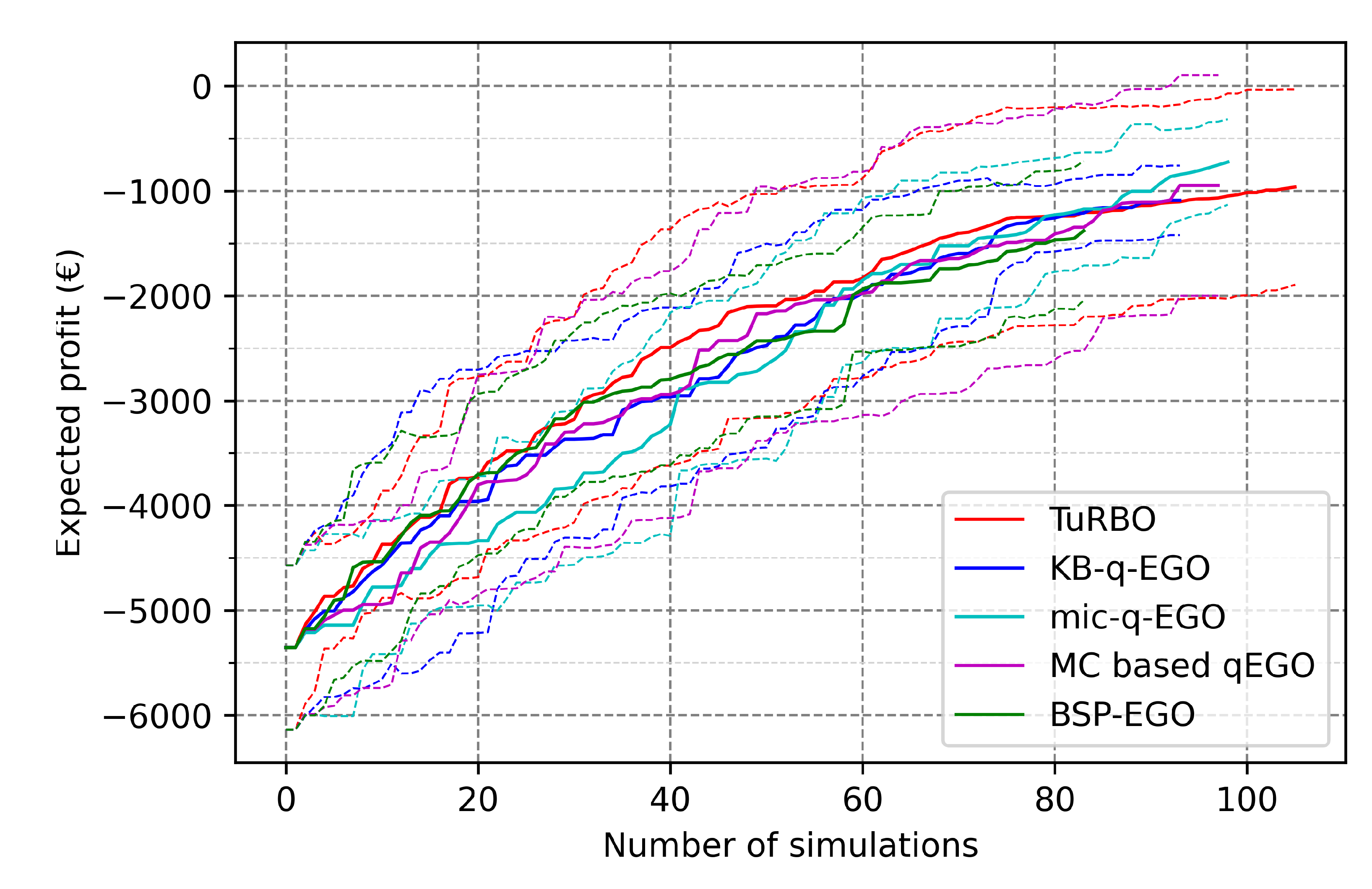
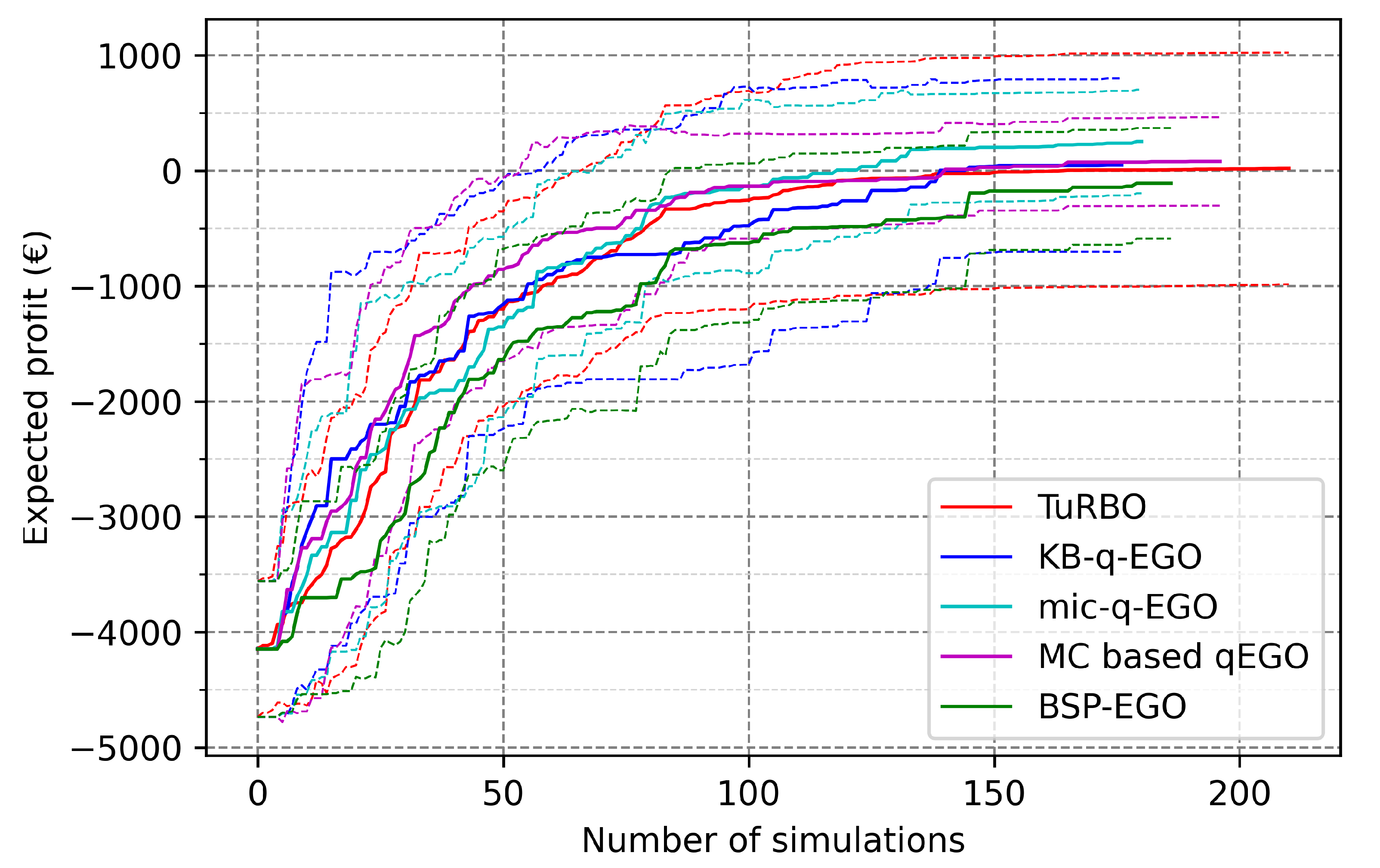
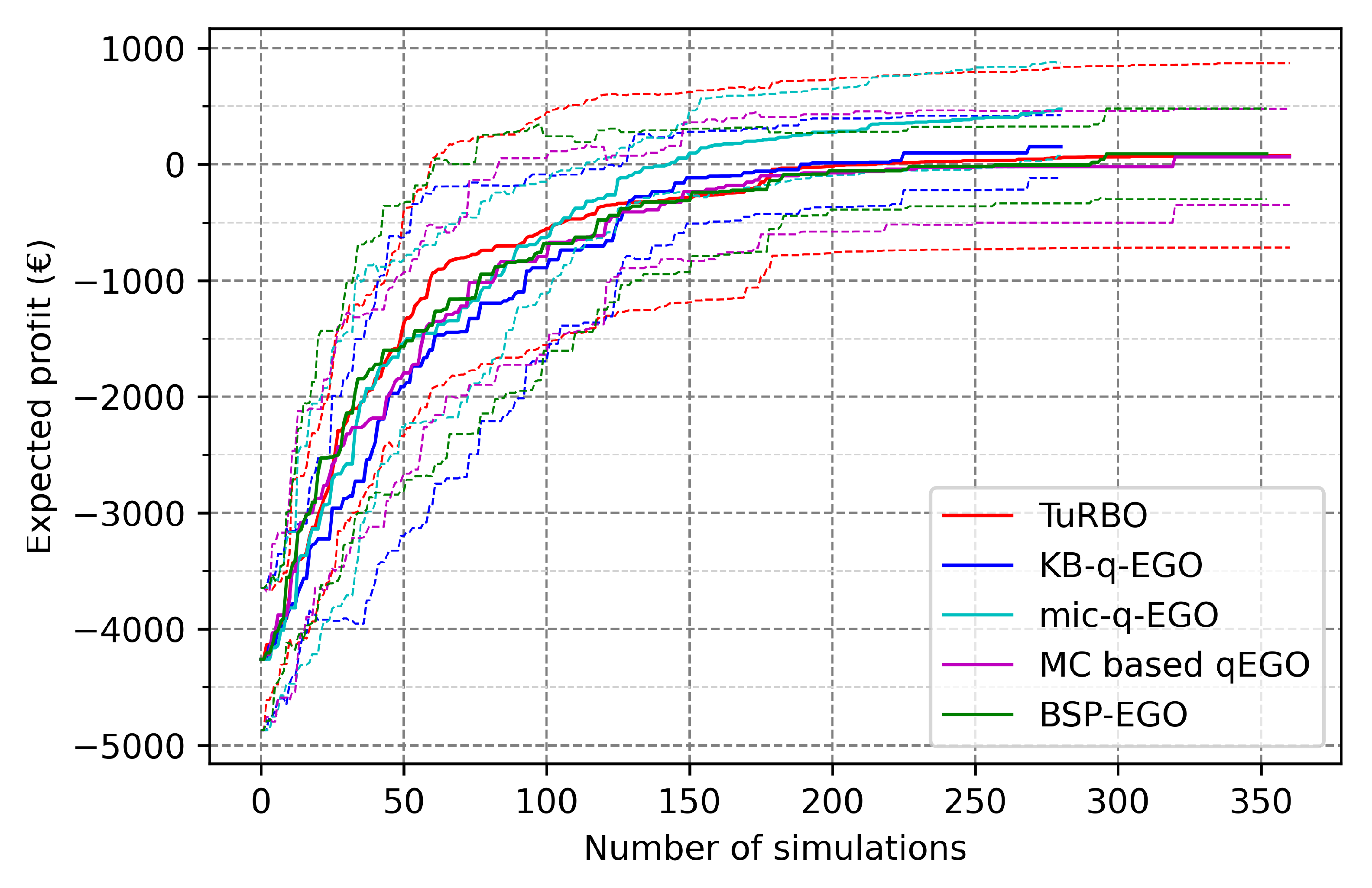
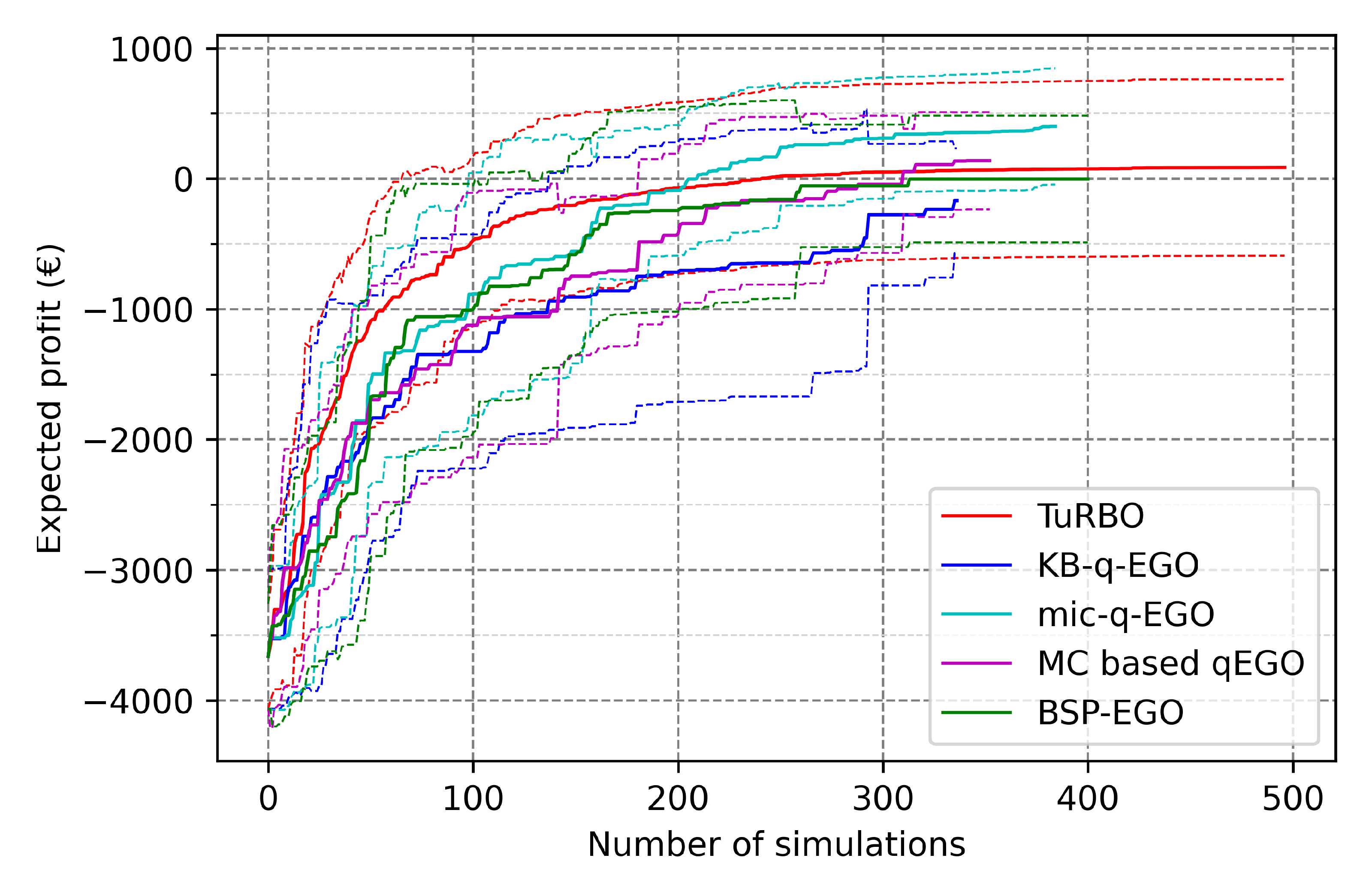
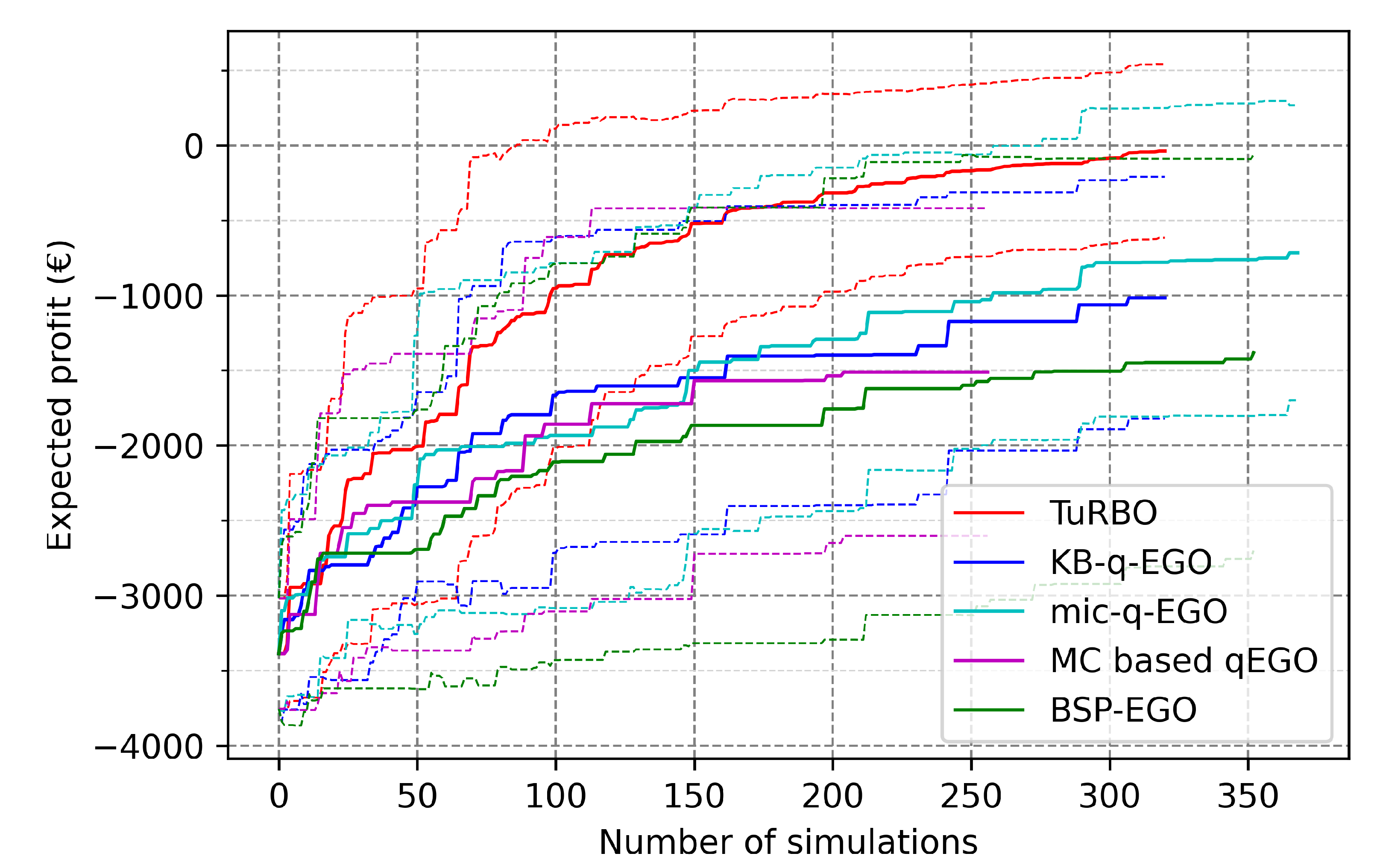
• The performance of a method in terms of the final outcome is compared to its contestants, for a fixed batch size. This is the main objective for the UPHES application: what is the best strategy to optimize the expected profit regarding the given optimization context?
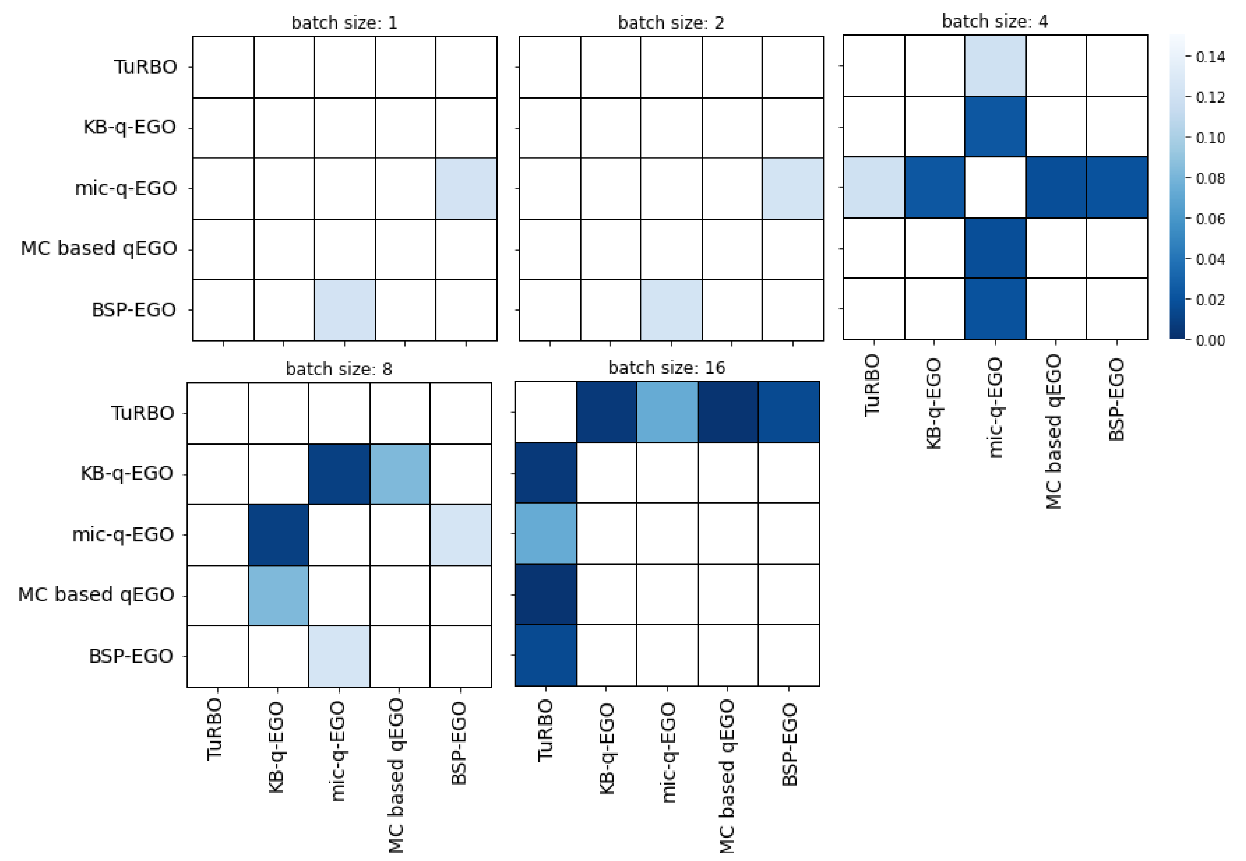
• The performance of the method in terms of the outcome in proportion to the batch size. Ideally, the method obtains equivalent quality of the outcome for an equivalent number of simulations, whatever the batch size. Thus, for a given number of cycles, we achieve better results when increasing the batch size.
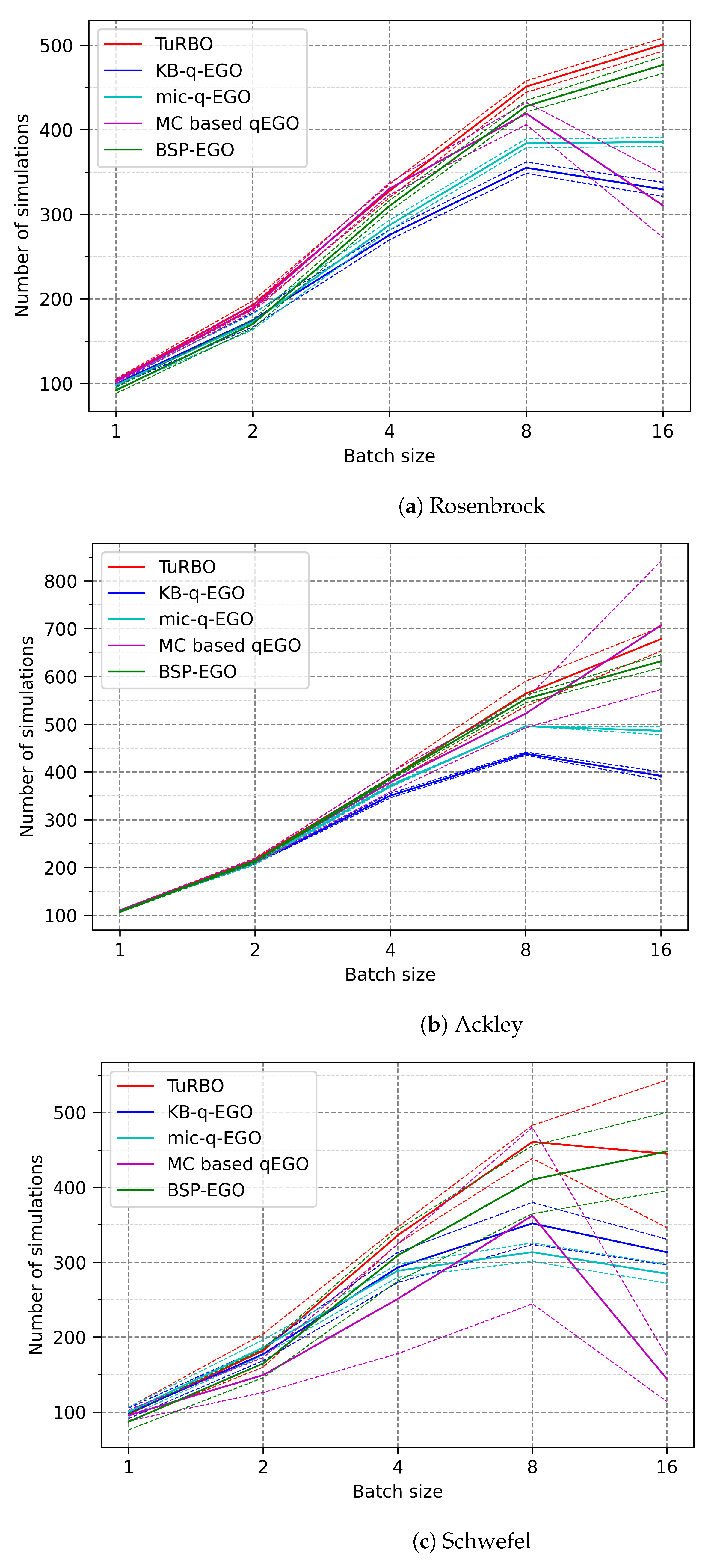
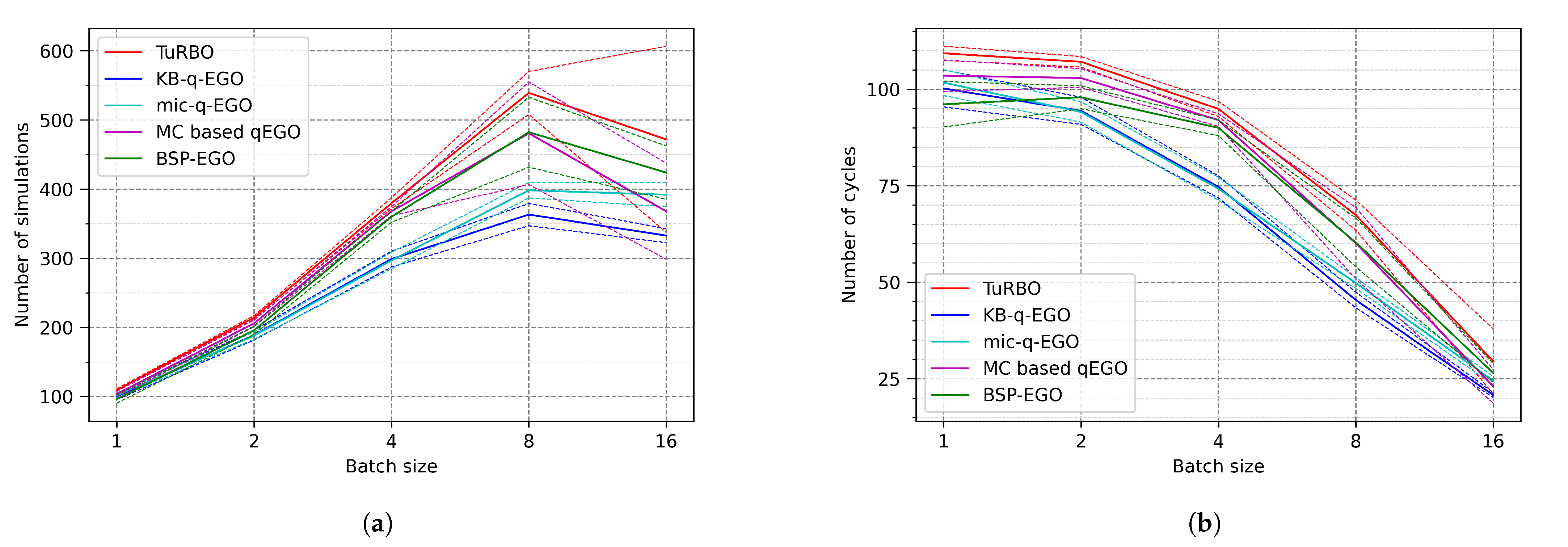
• The scalability of the method, studied with the number of total cycles/simulations performed in the fixed time. The maximum number of cycles is 120 since the budget is 20 min, and a simulation lasts 10 s. Assuming there is no cost for obtaining a batch of candidates, the total number of simulations should be $120\times n_{cores}$. The expected ideal behavior is that the time cost arising from optimization methods (outside simulation time) remains short enough not to hamper the optimization. Therefore, increasing $n_{cores}$ also increases the number of simulations by the end of the time budget. Additionally, if the previous point is respected, it should also improve the quality of the final result.

3.1. Benchmark Function Analysis

Table 4. Final results in terms of average ($\mu$) and standard deviation ($\sigma$) over 10 execution of each algorithm for the Rosenbrock benchmark function.

${\mathit{n}}_{\mathit{batch}}$	TuRBO		KB-q-EGO		mic-q-EGO		MC-q-EGO		BSP-EGO
	$\mathbf{\mu }$	$\mathbf{\sigma }$	$\mathbf{\mu }$	$\mathbf{\sigma }$	$\mathbf{\mu }$	$\mathbf{\sigma }$	$\mathbf{\mu }$	$\mathbf{\sigma }$	$\mathbf{\mu }$	$\mathbf{\sigma }$
1	1108	672	1538	735	1584	971	1362	665	1336	776
2	210	174	817	248	708	272	960	387	1185	509
4	99	93	461	169	409	217	878	327	497	123
8	39	34	502	139	371	126	733	454	318	127
16	14	2	440	213	559	273	318	200	434	205

,

Table 5. Final results in terms of average ($\mu$) and standard deviation ($\sigma$) over 10 execution of each algorithm for the Ackley benchmark function.

${\mathit{n}}_{\mathit{batch}}$	TuRBO		KB-q-EGO		mic-q-EGO		MC- q-EGO		BSP-EGO
	$\mathbf{\mu }$	$\mathbf{\sigma }$	$\mathbf{\mu }$	$\mathbf{\sigma }$	$\mathbf{\mu }$	$\mathbf{\sigma }$	$\mathbf{\mu }$	$\mathbf{\sigma }$	$\mathbf{\mu }$	$\mathbf{\sigma }$
1	2.421	0.350	5.582	0.515	5.027	0.991	6.607	0.807	4.761	0.931
2	0.881	0.620	5.302	1.149	4.895	0.871	6.018	0.772	4.589	0.915
4	0.123	0.327	5.137	1.345	2.660	0.195	6.115	1.403	4.330	1.274
8	0.110	0.330	4.143	0.693	2.025	0.353	4.001	0.749	4.004	0.518
16	0.337	0.708	3.378	1.826	1.634	0.479	2.884	0.457	2.882	0.482

and

Table 6. Final results in terms of average ($\mu$) and standard deviation ($\sigma$) over 10 execution of each algorithm for the Schwefel benchmark function.

${\mathit{n}}_{\mathit{batch}}$	TuRBO		KB-q-EGO		mic-q-EGO		MC- q-EGO		BSP-EGO
	$\mathbf{\mu }$	$\mathbf{\sigma }$	$\mathbf{\mu }$	$\mathbf{\sigma }$	$\mathbf{\mu }$	$\mathbf{\sigma }$	$\mathbf{\mu }$	$\mathbf{\sigma }$	$\mathbf{\mu }$	$\mathbf{\sigma }$
1	2229	345	2397	357	2605	317	2799	295	2693	306
2	1827	440	2652	129	2502	232	2689	422	2390	445
4	1767	459	2367	195	1775	489	2560	495	2182	340
8	1595	305	2579	312	2276	371	2411	396	2282	398
16	1660	323	2828	198	2489	328	2969	358	2409	215

display the average best cost obtained by each algorithm after 20 min of optimization, with an artificial 10 s simulation cost. Data are obtained with 10 independent executions, with 10 distinct initial sets used for all approaches. The first observation highlighted by the bold font in the tables is that TuRBO outperforms all the contestant methods for all batch sizes. Adding a complementary criterion in mic-q-EGO compared to KB-q-EGO seems to have a beneficial impact on final outcomes and achieves good performances for the Schwefel benchmark function. Regarding the standard deviations, TuRBO appears quite consistent in the final outcomes compared to other methods, except for the highly multi-modal Schwefel function. The latter observation about the Schwefel function and TuRBO is mitigated by the better average performance of the algorithm.

Figure 2a–c shows the number of simulations performed in 20 min as a function of the batch size. Since the evaluation time is the same, the difference is explained by the AP time (model learning excluded). A strong advantage of TuRBO is that its acquisition time is smaller than of other methods, it is observable in Figure 2 where we can see that TuRBO almost always performs more evaluations. However, it is also remarkable that increasing the batch size does not necessarily increase the number of evaluations in a fixed time. Indeed, the first explanation is that the data set is being supplemented with $n_{batch}$ new points at each cycle, and it quickly becomes time-consuming to fit the model to the data. In addition, querying $n_{batch}$ new candidates involves a bigger time cost when $n_{batch}$ is big. Those two factors explain what we could call a breaking point: increasing the number of processing units does not increase the number of simulations or improve the final outcomes. The breaking point is visible for any method around $n_{batch}=8$. This is critical since we know that the relevance of large batches of points is lower than smaller batches [8], and in this context, it is not compensated by more evaluations. Regarding Table 4, Table 5 and Table 6, the breaking point is noticeable by an increase in the average final cost when increasing the batch size. The latter observation is present for any approach, even TuRBO despite its good performance.

It has to be noted that optimizing multi-point AF can be time-consuming in some situations, with large batch sizes. For example, for Rosenbrock and Schwefel functions, the AP time cost is much higher than the one from the Ackley study and dominates the learning time cost. We observe in Figure 2 a clear decrease in the number of simulations for MC-based q-EGO which is not or less visible for TuRBO possibly thanks to its local AP inside a trust region which makes the inner optimization faster. Only BSP-EGO managed to achieve better scalability for the three studied functions in terms of function evaluation with respect to the batch size (i.e., the number of used cores in this study) thanks to its parallel AP using multiple single point EI. However and despite performances comparable to q-EGO-like methods, TuRBO performs better and manages to obtain very good final cost, probably because of its good intensification in the trust region. For larger batch sizes, e.g., $n_{batch}=16$, relying on sequential heuristics as in KB-q-EGO and mic-q-EGO or having a parallel AP such as in BSP-EGO can be a better choice for scalability compared to multi-points AF. The time cost of the inner optimization of q-EI is also unstable regarding the time needed to provide a batch of points, single point approaches are more predictable in terms of execution time as indicated by the smaller standard deviations in Figure 2a–c.

3.2. Application to UPHES Management

Results displayed in Figure 3, Figure 4, Figure 5, Figure 6 and Figure 7 present the average profit value of the UPHES management problem according to the number of simulations performed by the algorithms. Dashed lines are added to indicate the standard deviation around the average objective value. Optimization runs are repeated 10 times with 10 different initial sets, and each algorithm is run once with each initial set. Therefore, within each figure, every curve has the same starting point. Since the limiting factor is time, each execution of the optimization algorithms does not perform the same number of cycles (and simulations). Consequently, the curves only display the results for which all data are available, and the rest are truncated. Thereby, the final expected profit is not always visible on the graphs. Nevertheless, the final results at the end of the time budget are visible in

Table 7. Minimum, maximum, average profit values (EUR) as well as standard deviation of the UPHES management problem obtained with 10 runs of each method according to batch size.

${\mathit{n}}_{\mathit{batch}}=1$	min	mean	max	sd
TuRBO	−2469	−898	368	917
KB-q-EGO	−1582	−765	−27	416
mic-q-EGO	−1511	−609	−39	487
MC-based q-EGO	−2123	−690	108	778
BSP-EGO	−2248	−1126	139	883
${\mathit{n}}_{\mathit{batch}}=\mathbf{2}$	min	mean	max	sd
TuRBO	−2106	19	1338	1058
KB-q-EGO	−1474	167	1147	773
mic-q-EGO	−429	253	1369	473
MC-based q-EGO	−517	79	768	404
BSP-EGO	−708	−101	723	503
${\mathit{n}}_{\mathit{batch}}=\mathbf{4}$	min	mean	max	sd
TuRBO	−1766	78	819	837
KB-q-EGO	−344	168	784	287
mic-q-EGO	−96	559	1097	405
MC-based q-EGO	−548	65	824	436
BSP-EGO	−389	90	746	412
${\mathit{n}}_{\mathit{batch}}=\mathbf{8}$	min	mean	max	sd
TuRBO	−972	86	1259	713
KB-q-EGO	−703	−168	547	423
mic-q-EGO	−568	416	1184	473
MC-based q-EGO	−362	163	862	381
BSP-EGO	−1102	78	504	463
${\mathit{n}}_{\mathit{batch}}=\mathbf{16}$	min	mean	max	sd
TuRBO	−827	51	1162	692
KB-q-EGO	−2048	−963	658	752
mic-q-EGO	−2383	−706	684	1049
MC-based q-EGO	−2475	−1225	−14	948
BSP-EGO	−3509	−1183	408	1275

. The table also presents the minimum, maximum and standard deviation of each set of optimizations, for all batch sizes and all approaches.

First, looking at the average profit curves for batch sizes 1 and 2 in Figure 3 and Figure 4, we observe very few differences in the execution of the algorithms. The average values are similar, with maybe a thin advantage for the mic-q-EGO algorithm thanks to its smaller variance. Table 7 confirms the previous observation that mic-q-EGO performs slightly better in terms of average profit, and has the highest minimal expected profit among the 10 executions compared to other approaches. Then in this context, mic-q-EGO seems to be the safest choice. However, according to the p-value of the pairwise Student’s t-test summarized in Figure 8, no significant difference is observed (p-value > 0.1).

Regarding results for $n_{batch}=4$ in Figure 5, from around 150 iterations on, the mic-q-EGO appears to outperform the other approaches. With 150 simulations, the latter reaches a final expected profit equivalent to its competitors with twice as many simulations. Others are visually equivalent, with only a noticeable difference regarding the standard deviation. Indeed, as for the previously mentioned curves ($n_{batch}=1,2$), TuRBO has the highest variance. Except for mic-q-EGO, which has the highest minimum, average and maximum profit for $n_{batch}=4$, all the approaches have similar behavior and final outcomes. The advantage of mic-q-EGO is confirmed by the t-tests displayed in Figure 8 where a significant advantage for mic-q-EGO is visible. The p-value of comparison with KB-q-EGO, BSP-EGO and MC-based q-EGO is around 0.02 which provides strong evidence in favor of mic-q-EGO, while the comparison against TuRBO gives a p-value of 0.12 (less evidence, but strong assumption).

As for $n_{batch}=8$ (Figure 6), the difference between methods become cleaner, mic-q-EGO still provides better profit than contestant approaches or equivalent with half of the simulations, and in particular, better than KB-q-EGO which indicates that relying on a complementary AF efficiently improves the AP for larger batch sizes. However, the difference in final profit and standard deviation becomes smaller between methods, and no statistical difference can be observed in favor of a better average profit for mic-q-EGO against all others.

Finally, Figure 7 clearly illustrates different behaviors of the investigated algorithm when increasing the batch size to 16. While BSP-EGO and MC-based q-EGO have similar performances, the three remaining have not. Classical KB-q-EGO is again on average less efficient than its multi-criteria counterpart, and both of them are significantly ($p<0.1$) different from TuRBO.

Looking at the final objective values in Table 7, we observe an improvement of the final average and worst-case profit, along with the increase of the batch size up to $n_{batch}=4$. Nevertheless, similar values are observed for $n_{batch}=8$ compared to $n_{batch}=4$, despite the larger batch size and higher number of simulations. Additionally, regarding results with $n_{batch}=16$, we observe a clear deterioration of the final outcomes except for TuRBO results which remain equivalent to $n_{batch}=8$. The breaking point defined in the benchmark analysis is clearly visible also for the UPHES application. Except for TuRBO, $n_{batch}=4$ seems to be the best compromise between speed of execution and quality of the candidates provided by the AP. Either by improving the average profit, the minimum value of profit, or reducing variance, TuRBO benefits from a larger batch size. Even though TuRBO is the only method managing to improve the quality of the final outcomes when increasing the batch size, it does not compete with mic-q-EGO ($n_{batch}=4$) at any batch size.

To put these observations into perspective, consider Figure 9a,b, which shows the number of cycles (resp. simulations) performed in the dedicated time as a function of the batch size. The latter indicates how efficiently the algorithms use parallel processing capabilities. In accordance with the observations of the benchmark section, all algorithms reach a breaking point between $n_{batch}=8$ and $n_{batch}=16$, which results in a clear loss in the final profits (see Table 7).

More precisely, looking at Figure 9b, we can see that the number of cycles for $n_{batch}=1$ or $n_{batch}=2$ is equivalent, and close enough to the maximum of 120 in both cases. It must be noted that for those batch sizes, TuRBO achieves almost 110 cycles and is the fastest method of our test bed. It can be observed as well in Figure 3 and Figure 4 where the TuRBO curve continues beyond other curves. The quickness of TuRBO compared to MC-based q-EGO, which are using the same inner optimization, can be explained by the smaller search space: TuRBO focuses on a trust region.

Increasing the batch size to 4 makes the conceptual differences between algorithms appear. Indeed, we can see that sequential AP heuristics of q-EGO like algorithms are quite time-consuming compared to APs of TuRBO and MC-based q-EGO. Even if BSP-EGO carries out $2\times n_{batch}$ sub-APs, its parallel execution makes it as fast as MC-based q-EGO. Although the number of cycles is slightly smaller than for lower batch sizes, it is the best compromise regarding final expected profits of Table 7.

Reaching $n_{batch}=8$ allows to perform more simulations for any method, but at the cost of the number of cycles. The productivity per computing core is clearly diminished and as suggested by the final profits, it is not profitable in this context except maybe for TuRBO. Finally, consistently with benchmark section observations, the significant decrease in the number of cycles involves a drop in the number of simulations which is almost comparable to $n_{batch}=4$. Nevertheless, as suggested in the BOTorch documentation [12], the gap between sequential heuristics and MC-based AF becomes smaller for large batch sizes because of the complexity of multi-points AF optimization. In addition, it has to be noted that relying on different single point AF, as in mic-q-EGO is efficient to reduce the acquisition time and to improve the quality of the batch of candidates for large batch sizes.

4. Discussion

Both benchmark analysis and UPHES management application highlight conceptual differences between algorithms, especially regarding their behavior when increasing the batch size. Using PBO in a time-restricted setting necessitates to take into account the quickly increasing time needed to fit a surrogate model and to optimize the acquisition function. Our experiments have indeed shown that there is a “breaking point” beyond which an increase in the batch size deteriorates performance instead of adding value to the optimization process. Generally speaking, the breaking point in our context appears between $n_{batch}=4$ and $n_{batch}=16$, depending on the algorithm and the objective function. Indeed, the landscape of the optimized function impacts the model learning time and the acquisition time. This becomes clear when looking at the number of simulations achieved in a fixed amount of time for the three benchmark functions (Figure 2a–c). The Schwefel function is highly multi-modal with mode values of the same amplitude, hence, the greater time cost of AP compared to the Ackley function, where the minimum value area can be identified clearly. The breaking point is reached faster given that the learning time and acquisition time are significant.

The addition of a complementary criterion (i.e., mic-q-EGO using UCB and EI) is efficient to obtain better outcomes in this situation in comparison with KB-q-EGO. However, the main bottleneck being the global model fitting, the breaking point is only slightly delayed thanks to the smaller number of model updates compared to KB-q-EGO. The mic-q-EGO approach is not suited for large batch sizes either. Regarding the number of performed simulations in Figure 9, we can conclude similarly: despite a faster AP of mic-q-EGO, the global model remains restricting. The same conclusion can be drawn for any approach using global models, fitted on the full data set.

Another characteristic of the investigated APs is the search space decomposition. On the one side, TuRBO focuses on a trust region and we observed a significant impact on AP execution speed, as well as a clear advantage in convergence towards better outcomes, especially for benchmark functions. On the other side, BSP-EGO exploits space decomposition in the service of parallel computing. The gain in execution time allows multiplying the number of sub-regions so that each computing core is in charge of two sub-regions, yielding $2\times n_{batch}$ candidates before selecting $n_{batch}$ for evaluation. In both cases, the total number of evaluations is increased compared to other approaches thanks to space partitioning.

For the UPHES management problem, the final expected profit is considerably improved compared to the initial sampling thanks to PBO. Even considering a large random sample of almost 12,000 objective function evaluations, the best-observed profit is around EUR −1200. All investigated BO algorithms allow to achieve much better profits with significantly fewer simulations. This demonstrates the need for efficient optimization algorithms for this application.

The latter observations allow extracting some general recommendations regarding BO within restricted time. Firstly, the surrogate model should remain fast to train even with a large data set. If it becomes excessively time-consuming, one can use subsets of data, or even rely on different models faster to fit: Bayesian Neural Networks [47], Sparse GP and variational inference [48], Ensemble Methods using additive structures of GPs [49] or low rank approximations of the Gram matrix [50]. Secondly, AP must also remain fast enough. In some cases AP time can become larger than learning and simulation time (for instance in MC-based q-EGO) and considerably reduce the number of possible cycles in a given time. Using multiple criteria has proven its efficiency in this study, and might be further experimented with more AFs as in Li et al. [51] Finally, possibly effective to speed up both the fitting of the model and the AP, space partitioning appears to be a judicious choice. Both TuRBO and BSP-EGO reduce acquisition time, and other methods such as Villanueva et al. [52] and Wang et al. [53] present advantages for parallel computing and convergence. Combining the strength of the different approaches remains to be investigated. For example, a multi-infill-criterion TuRBO can easily be considered and implemented.

5. Conclusions and Future Research Directions

Five batch-acquisition Bayesian Optimization (BO) algorithms are investigated in this study with the objective of identifying the most suited approach for maximizing the profit of an Underground Pumped Hydro-Energy Storage (UPHES) operator. The profit is given by a simulator computing the expected profit according to a set of decisions. The latter evaluation of a decision vector lasts 10 s, and the optimization must be completed in 20 min (initial sampling excluded). These constraints place us in the context of black-box optimization with a time-consuming simulator, except that the simulator is time-consuming in regards to the time constraint. Therefore, unlike the classical BO assumption, learning and acquisition time are not negligible.

The study reveals that in this context, as well as on benchmark problems than on the UPHES management problem, resorting to large batch sizes and large parallelization quickly becomes excessively time-consuming, worsening the performance of any BO algorithm considered in this work. The best compromise lies between batch sizes of 4 and 8. Best performances are achieved by the TrUst Region BO algorithm (TuRBO) with $n_{batch}=8$ in case of benchmark function, whereas q-EGO with multi-infill criteria sampling (mic-q-EGO) and $n_{batch}=4$ performs best in the UPHES context. Parallel BO algorithms manage to find consistently good solutions to the UPHES management problem and appear as a viable way to approach time-constrained applications despite the high overhead incurred by surrogate management. However, making the most of parallel computing in this context remains challenging.

Finally, some general leads are discussed to overcome the scalability issues. Using fast-to-fit surrogate models, multiple complementary criteria and space partitioning (or space reduction) might considerably improve the performance of surrogate-guided optimization in the context of UPHES optimization.

References

1. Toubeau, J.F.; Bottieau, J.; De Grève, Z.; Vallée, F.; Bruninx, K. Data-Driven Scheduling of Energy Storage in Day-Ahead Energy and Reserve Markets With Probabilistic Guarantees on Real-Time Delivery. IEEE Trans. Power Syst. 2021, 36, 2815–2828. [Google Scholar] [CrossRef]
2. Gobert, M.; Gmys, J.; Toubeau, J.F.; Vallée, F.; Melab, N.; Tuyttens, D. Surrogate-Assisted Optimization for Multi-stage Optimal Scheduling of Virtual Power Plants. In Proceedings of the 2019 International Conference on High Performance Computing Simulation (HPCS), Dublin, Ireland, 15–19 July 2019; pp. 113–120. [Google Scholar] [CrossRef]
3. Toubeau, J.F.; De Grève, Z.; Goderniaux, P.; Vallée, F.; Bruninx, K. Chance-Constrained Scheduling of Underground Pumped Hydro Energy Storage in Presence of Model Uncertainties. IEEE Trans. Sustain. Energy 2020, 11, 1516–1527. [Google Scholar] [CrossRef]
4. Taktak, R.; D’Ambrosio, C. An overview on mathematical programming approaches for the deterministic unit commitment problem in hydro valleys. Energy Syst. 2017, 8, 57–79. [Google Scholar] [CrossRef]
5. Steeger, G.; Barroso, L.; Rebennack, S. Optimal Bidding Strategies for Hydro-Electric Producers: A Literature Survey. IEEE Trans. Power Syst. 2014, 29, 1758–1766. [Google Scholar] [CrossRef]
6. Shahriari, B.; Swersky, K.; Wang, Z.; Adams, R.P.; de Freitas, N. Taking the Human Out of the Loop: A Review of Bayesian Optimization. Proc. IEEE 2016, 104, 148–175. [Google Scholar] [CrossRef] [Green Version]
7. Haftka, R.; Villanueva, D.; Chaudhuri, A. Parallel surrogate-assisted global optimization with expensive functions—A survey. Struct. Multidiscip. Optim. 2016, 54, 3–13. [Google Scholar] [CrossRef] [Green Version]
8. Briffoteaux, G.; Gobert, M.; Ragonnet, R.; Gmys, J.; Mezmaz, M.; Melab, N.; Tuyttens, D. Parallel surrogate-assisted optimization: Batched Bayesian Neural Network-assisted GA versus q-EGO. Swarm Evol. Comput. 2020, 57, 100717. [Google Scholar] [CrossRef]
9. Ginsbourger, D.; Le Riche, R.; Carraro, L. A Multi-points Criterion for Deterministic Parallel Global Optimization Based on Gaussian Processes; Technical report; Ecole Nationale Suṕerieure des Mines: Saint-Etienne, France, 2008. [Google Scholar]
10. Liu, J.; Song, W.; Han, Z.H.; Zhang, Y. Efficient aerodynamic shape optimization of transonic wings using a parallel infilling strategy and surrogate models. Struct. Multidiscip. Optim. 2017, 55, 925–943. [Google Scholar] [CrossRef]
11. Wang, Y.; Han, Z.H.; Zhang, Y.; Song, W. Efficient Global Optimization using Multiple Infill Sampling Criteria and Surrogate Models. In Proceedings of the 2018 AIAA Aerospace Sciences Meeting, Kissimmee, FL, USA, 8–12 January 2018. [Google Scholar] [CrossRef]
12. Balandat, M.; Karrer, B.; Jiang, D.R.; Daulton, S.; Letham, B.; Wilson, A.G.; Bakshy, E. BoTorch: A Framework for Efficient Monte-Carlo Bayesian Optimization. Adv. Neural Inf. Process. Syst. 2020, 33, 21524–21538. [Google Scholar]
13. Gobert, M.; Gmys, J.; Melab, N.; Tuyttens, D. Adaptive Space Partitioning for Parallel Bayesian Optimization. In Proceedings of the HPCS 2020—The 18th International Conference on High Performance Computing Simulation, Barcelona, Spain, 20–27 March 2021. [Google Scholar]
14. Eriksson, D.; Pearce, M.; Gardner, J.R.; Turner, R.; Poloczek, M. Scalable Global Optimization via Local Bayesian Optimization. arXiv 2020, arXiv:cs.LG/1910.01739. [Google Scholar]
15. Abreu, L.V.L.; Khodayar, M.E.; Shahidehpour, M.; Wu, L. Risk-Constrained Coordination of Cascaded Hydro Units with Variable Wind Power Generation. IEEE Trans. Sustain. Energy 2012, 3, 359–368. [Google Scholar] [CrossRef]
16. Toubeau, J.F.; De Grève, Z.; Vallée, F. Medium-Term Multimarket Optimization for Virtual Power Plants: A Stochastic-Based Decision Environment. IEEE Trans. Power Syst. 2018, 33, 1399–1410. [Google Scholar] [CrossRef]
17. Montero, R.; Wortberg, T.; Binias, J.; Niemann, A. Integrated Assessment of Underground Pumped-Storage Facilities Using Existing Coal Mine Infrastructure. In Proceedings of the 4th IAHR Europe Congress, Liege, Belgium, 27–29 July 2016; pp. 953–960. [Google Scholar]
18. Pujades, E.; Orban, P.; Bodeux, S.; Archambeau, P.; Erpicum, S.; Dassargues, A. Underground pumped storage hydropower plants using open pit mines: How do groundwater exchanges influence the efficiency? Appl. Energy 2017, 190, 135–146. [Google Scholar] [CrossRef]
19. Ponrajah, R.; Witherspoon, J.; Galiana, F. Systems to Optimize Conversion Efficiencies at Ontario Hydro’s Hydroelectric Plants. IEEE Trans. Power Syst. 1998, 13, 1044–1050. [Google Scholar] [CrossRef]
20. Pannatier, Y. Optimisation des Stratégies de Réglage d’une Installation de Pompage-Turbinage à Vitesse Variable; EPFL: Lausanne, Switzerland, 2010. [Google Scholar] [CrossRef]
21. Toubeau, J.F.; Iassinovski, S.; Jean, E.; Parfait, J.Y.; Bottieau, J.; De Greve, Z.; Vallee, F. A Nonlinear Hybrid Approach for the Scheduling of Merchant Underground Pumped Hydro Energy Storage. IET Gener. Transm. Distrib. 2019, 13, 4798–4808. [Google Scholar] [CrossRef]
22. Cheng, C.; Wang, J.; Wu, X. Hydro Unit Commitment With a Head-Sensitive Reservoir and Multiple Vibration Zones Using MILP. IEEE Trans. Power Syst. 2016, 31, 4842–4852. [Google Scholar] [CrossRef]
23. Arce, A.; Ohishi, T.; Soares, S. Optimal dispatch of generating units of the Itaipu hydroelectric plant. IEEE Trans. Power Syst. 2002, 17, 154–158. [Google Scholar] [CrossRef]
24. Catalao, J.P.S.; Mariano, S.J.P.S.; Mendes, V.M.F.; Ferreira, L.A.F.M. Scheduling of Head-Sensitive Cascaded Hydro Systems: A Nonlinear Approach. IEEE Trans. Power Syst. 2009, 24, 337–346. [Google Scholar] [CrossRef]
25. Chen, P.H.; Chang, H.C. Genetic aided scheduling of hydraulically coupled plants in hydro-thermal coordination. IEEE Trans. Power Syst. 1996, 11, 975–981. [Google Scholar] [CrossRef]
26. Yu, B.; Yuan, X.; Wang, J. Short-term hydro-thermal scheduling using particle swarm optimization method. Energy Convers. Manag. 2007, 48, 1902–1908. [Google Scholar] [CrossRef]
27. Kushner, H.J. A New Method of Locating the Maximum Point of an Arbitrary Multipeak Curve in the Presence of Noise. J. Fluids Eng. 1964, 86, 97–106. [Google Scholar] [CrossRef]
28. Mockus, J.; Tiesis, V.; Zilinskas, A. The Application of Bayesian Methods for Seeking the Extremum; Towards Global Optimization: Berlin, Germany, 2014; Volume 2, pp. 117–129. [Google Scholar]
29. Jones, D.R.; Schonlau, M.; Welch, W.J. Efficient Global Optimization of Expensive Black-Box Functions. J. Glob. Optim. 1998, 13, 455–492. [Google Scholar] [CrossRef]
30. Srinivas, N.; Krause, A.; Kakade, S.; Seeger, M. Gaussian Process Optimization in the Bandit Setting: No Regret and Experimental Design. arXiv 2010, arXiv:0912.3995. [Google Scholar]
31. Močkus, J. On bayesian methods for seeking the extremum. In Proceedings of the Optimization Techniques IFIP Technical Conference, Novosibirsk, Russia, 1–7 July 1974; Marchuk, G.I., Ed.; Springer: Berlin/Heidelberg, Germany, 1975; pp. 400–404. [Google Scholar]
32. Noè, U.; Husmeier, D. On a New Improvement-Based Acquisition Function for Bayesian Optimization. arXiv 2018, arXiv:abs/1808.06918. [Google Scholar]
33. Hennig, P.; Schuler, C. Entropy Search for Information-Efficient Global Optimization. J. Mach. Learn. Res. 2011, 13, 1809–1837. [Google Scholar]
34. Hernández-Lobato, J.M.; Hoffman, M.W.; Ghahramani, Z. Predictive Entropy Search for Efficient Global Optimization of Black-box Functions. In Proceedings of the Advances in Neural Information Processing Systems, Montreal, QC, Canada, 8–13 December 2014; Volume 27, pp. 1–6. [Google Scholar]
35. Wang, Z.; Jegelka, S. Max-value Entropy Search for Efficient Bayesian Optimization. In Proceedings of the 34th International Conference on Machine Learning, Sydney, Australia, 6–11 August 2017; Volume 70, pp. 3627–3635. [Google Scholar]
36. Ginsbourger, D.; Riche, R.L.; Carraro, L. Kriging Is Well-Suited to Parallelize Optimization; Springer: Berlin/Heidelberg, Germany, 2010. [Google Scholar]
37. González, J.; Dai, Z.; Hennig, P.; Lawrence, N.D. Batch Bayesian Optimization via Local Penalization. arXiv 2015, arXiv:stat.ML/1505.08052. [Google Scholar]
38. Zhan, D.; Qian, J.; Cheng, Y. Balancing global and local search in parallel efficient global optimization algorithms. J. Glob. Optim. 2017, 67, 873–892. [Google Scholar] [CrossRef]
39. Palma, A.D.; Mendler-Dünner, C.; Parnell, T.; Anghel, A.; Pozidis, H. Sampling Acquisition Functions for Batch Bayesian Optimization. arXiv 2019, arXiv:cs.LG/1903.09434. [Google Scholar]
40. Lyu, W.; Yang, F.; Yan, C.; Zhou, D.; Zeng, X. Batch Bayesian Optimization via Multi-objective Acquisition Ensemble for Automated Analog Circuit Design. In Proceedings of the 35th International Conference on Machine Learning, Stockholm, Sweden, 10–15 July 2018; Dy, J., Krause, A., Eds.; Proceedings of Machine Learning Research; PMLR: Stockholm Sweden, 2018; Volume 80, pp. 3306–3314. [Google Scholar]
41. Feng, Z.; Zhang, Q.; Zhang, Q.; Tang, Q.; Yang, T.; Ma, Y. A multiobjective optimization based framework to balance the global exploration and local exploitation in expensive optimization. J. Glob. Optim. 2014, 61, 677–694. [Google Scholar] [CrossRef]
42. Rasmussen, C.E.; Williams, C.K.I. Gaussian Processes for Machine Learning (Adaptive Computation and Machine Learning); The MIT Press: Cambridge, MA, USA, 2005. [Google Scholar]
43. Wilson, J.T.; Moriconi, R.; Hutter, F.; Deisenroth, M.P. The reparameterization trick for acquisition functions. arXiv 2017, arXiv:1712.00424. [Google Scholar]
44. Artiba, A.; Emelyanov, V.; Iassinovski, S. Introduction to Intelligent Simulation: The RAO Language. J. Oper. Res. Soc. 2000, 51, 395–515. [Google Scholar] [CrossRef]
45. Surjanovic, S.; Bingham, D. Virtual Library of Simulation Experiments: Test Functions and Datasets. Available online: http://www.sfu.ca/~ssurjano (accessed on 13 October 2022).
46. Dalcin, L.; Fang, Y.L.L. mpi4py: Status Update After 12 Years of Development. Comput. Sci. Eng. 2021, 23, 47–54. [Google Scholar] [CrossRef]
47. Lin, X.; Zhen, H.L.; Li, Z.; Zhang, Q.; Kwong, S. A Batched Scalable Multi-Objective Bayesian Optimization Algorithm. arXiv 2018, arXiv:1811.01323. [Google Scholar]
48. Leibfried, F.; Dutordoir, V.; John, S.; Durrande, N. A Tutorial on Sparse Gaussian Processes and Variational Inference. arXiv 2020, arXiv:2012.13962. [Google Scholar] [CrossRef]
49. Wang, Z.; Gehring, C.; Kohli, P.; Jegelka, S. Batched Large-scale Bayesian Optimization in High-dimensional Spaces. arXiv 2017, arXiv:1706.01445. [Google Scholar]
50. Solin, A.; Särkkä, S. Hilbert Space Methods for Reduced-Rank Gaussian Process Regression. Stat. Comput. 2020, 30, 419–446. [Google Scholar] [CrossRef] [Green Version]
51. Li, Z.; Ruan, S.; Gu, J.; Wang, X.; Shen, C. Investigation on parallel algorithms in efficient global optimization based on multiple points infill criterion and domain decomposition. Struct. Multidiscip. Optim. 2016, 54, 747–773. [Google Scholar] [CrossRef]
52. Villanueva, D.; Le Riche, R.; Picard, G.; Haftka, R. Dynamic Design Space Partitioning for Optimization of an Integrated Thermal Protection System. In Proceedings of the 54th AIAA/ASME/ASCE/AHS/ASC Structures, Structural Dynamics, and Materials Conference, Boston, MA, USA, 8–11 April 2013. [Google Scholar] [CrossRef] [Green Version]
53. Wang, G.; Simpson, T. Fuzzy clustering based hierarchical metamodeling for design space reduction and optimization. Eng. Optim. 2004, 36, 313–335. [Google Scholar] [CrossRef]
Figure 1. Topology of the modeled PSH unit on Maizeret site [21].
Algorithms 15 00446 g001
Figure 2. Number of function evaluations as a function of the batch size. Solid lines indicate the average over 10 runs, and dashed lines of same colors indicate the standard deviation.
Algorithms 15 00446 g002
Figure 3. Evolution of the best-known objective value according to the number of executed cycles with n b a t c h = 1 . Solid lines indicate the average over 10 runs, and dashed lines of same colors indicate the standard deviation.
Algorithms 15 00446 g003
Figure 4. Evolution of the best-known objective value according to the number of executed cycles with n b a t c h = 2 . Solid lines indicate the average over 10 runs, and dashed lines of same colors indicate the standard deviation.
Algorithms 15 00446 g004
Figure 5. Evolution of the best-known objective value according to the number of executed cycles with n b a t c h = 4 . Solid lines indicate the average over 10 runs, and dashed lines of same colors indicate the standard deviation.
Algorithms 15 00446 g005
Figure 6. Evolution of the best-known objective value according to the number of executed cycles with n b a t c h = 8 . Solid lines indicate the average over 10 runs, and dashed lines of same colors indicate the standard deviation.
Algorithms 15 00446 g006
Figure 7. Evolution of the best known objective value according to the number of executed cycles with n b a t c h = 16 . Solid lines indicate the average over 10 runs, and dashed lines of same colors indicate the standard deviation.
Algorithms 15 00446 g007
Figure 8. Heatmap of the p-values of pairwise Student’s t-tests.
Algorithms 15 00446 g008
Figure 9. Study on the scalability of each approach. Solid lines indicate the average over 10 runs, and dashed lines of same colors indicate the standard deviation. (a) Number of simulations as a function of the batch size. (b) Number of cycles as a function of the batch size.
Algorithms 15 00446 g009