Article

Physics-Informed Neural Networks (PINNs)-Based Traffic State Estimation: An Application to Traffic Network

Department of Civil and Environmental Engineering, The University of Alabama in Huntsville, Huntsville, AL 35899, USA
*
Author to whom correspondence should be addressed.
Algorithms 2022, 15(12), 447; https://doi.org/10.3390/a15120447
Submission received: 18 October 2022 / Revised: 24 November 2022 / Accepted: 25 November 2022 / Published: 27 November 2022
(This article belongs to the Special Issue Neural Network for Traffic Forecasting)

Abstract

:
Traffic state estimation (TSE) is a critical component of the efficient intelligent transportation systems (ITS) operations. In the literature, TSE methods are divided into model-driven methods and data-driven methods. Each approach has its limitations. The physics information-based neural network (PINN) framework emerges to mitigate the limitations of the traditional TSE methods, while the state-of-art of such a framework has focused on single road segments but can hardly deal with traffic networks. This paper introduces a PINN framework that can effectively make use of a small amount of observational speed data to obtain high-quality TSEs for a traffic network. Both model-driven and data-driven components are incorporated into PINNs to combine the advantages of both approaches and to overcome their disadvantages. Simulation data of simple traffic networks are used for studying the highway network TSE. This paper demonstrates how to solve the popular LWR physical traffic flow model with a PINN for a traffic network. Experimental results confirm that the proposed approach is promising for estimating network traffic accurately.

1. Introduction

The traffic conditions on road segments in a network are usually described by macroscopic traffic state variables, such as flow rate, vehicle speed, and vehicle density as traffic streams. Transport planners identify congestion levels and traffic demands, as well as bottlenecks on roadways, through these indicators [1]. However, these important measurements are not available for all locations or times due to physical and budget constraints of the measurements; even if the availability issue is not a concern, undesired noises in the measurements have been making ITS traffic management operations difficult [2]. Combining factors such as the cost of sensor installation, the accuracy of vehicle detection techniques, and restrictions on data storage and transmission can often lead to partial observations of traffic state variables [3]. To deliver effective traffic management, it is vital to estimate traffic state variables at locations without sensor data.
Traffic state estimation (TSE) refers to the prediction of traffic state variables such as flow, density, and speed of road segments using partially observed traffic data [4]. Approaches to TSE can be roughly categorized into two groups based on the a priori knowledge they depend on: model-driven and data-driven. In model-driven approaches, traffic flow state predictions are based on prior knowledge of the flow, usually embodied in physics-based models such as the Lighthill–Whitham–Richards (LWR) model or the Aw–Rascle–Zhang (ARZ) model [5,6]. Physical processes play a key role in how these models work, such as the way the state variable changes across space and time. These models are much less limited by data availability and can make predictions without the training data. A model-based approach assumes that the physics-based models are representative of traffic dynamics and can be utilized to determine unobserved values based on partially observed data. Despite the independence from data requirements, the physics-based models suffer from a few challenges that may lead to low-quality estimates. Some of these challenges include: (i) they can only capture a limited set of traffic dynamics in real-world situations; (ii) they are derived under ideal conditions, entail large effort for parameter calibrations; and (iii) they are difficult to apply with noisy/fluctuating traffic data. The other group of TSE methods is the data-driven models based on machine learning. Data-driven models employ statistical relationships in data and are model-free so that formulating specific underlying physics is not necessary. Data-driven methods have been intensively studied recently due to the increasing availability of data, as they do not require specific theoretical assumptions and have a remarkably low computing cost during the testing phase. However, the data-driven nature of those machine learning (ML) models leaves them vulnerable to the following situations: (i) insufficient training data to learn the system’s complexity, (ii) training samples with misleading information, and (iii) test samples that are not representative of the training samples. Dramatic performance drops alongside large and/or biased estimations are not rare in these scenarios, which unfortunately are very common in the real world. In addition, the machine learning models are difficult to interpret because of their ‘black-box’ nature.
Very recent studies on the hybrid approaches integrate physics knowledge from traffic flow models and machine learning models, in order to mitigate the limitations of the above-mentioned approaches. For instance, Yuan et al. (2021) presented the physics regularized Gaussian process (PRGP) method for TSE by integrating macroscopic traffic flow models with Gaussian process (GP) [7]. Raissi et al. were the first ones to propose implementations of fully connected neural networks that incorporate residuals from partial differential equations (PDEs) into their loss function as regularizers, which restrains the feasible solution space [8]. The major advantage of physics-informed learning (PIL) is that an effective loss function can be implemented using a modest amount of data. However, there is a major limitation to using PIL: their high training costs can cause adverse effects on their performance, which is especially of concern when dealing with real-world applications. Using the domain decomposition approach, Jagtap and Karniadakis (2020) accelerated the convergence of these models without compromising their performance by partitioning the computational domain into more than one subdomain, and then defining boundaries between these subdomains that are subject to some continuity conditions [9]. The presented numerical experiments were, however, limited to the partitioning of a single solution space, which is not representative of the network’s links in a true sense. In a traffic network, the state variables are correlated with the physical characteristics of the links for example number of lanes, road geometry, etc. The existing PIL studies consider the training data from the exact solution space of the governing partial differential equation. The macroscopic traffic state variables, on the other hand, are estimated through sensors and are subject to various measurement biases and approximations. Therefore, the real or simulated traffic data does not strictly follow the traffic governing physics model.
Another limitation of the existing hybrid studies for training neural networks is that they mainly consider the exact solution of the traffic flow model over a spatiotemporal space subject to relevant initial and boundary conditions. Such an approach with the exact analytical solution may lead to two potential shortcomings: (1) the analytical solution of PDE contains negative traffic state variables, which is not realistic; (2) the data generated from a continuous road segment cannot have any merging or diverging points. Such deficiency is critical for a real-world traffic network, as the traffic dynamics with and without the network consideration are significantly different. The state-of-art of the hybrid models are only applicable to one road segment or a sequence of segments without merges or divergences, which greatly limits their applications. It is therefore imperative that such studies be extended to realistic road networks.
This study aims to fill the above research gaps by extending physics-informed neural network application to simulated traffic network data following the domain decomposition approach. In a domain decomposition approach, we divide the whole traffic network into individual links. Afterwards, the individual links are joined together (stitching process) corresponding to their connectivity in the network. The flow conservation condition is applied at the joints (merge/diverge sections) while stitching the link. The domain decomposition in the framework is very useful in three major aspects. First, different physical properties on different links in a traffic network can be properly modeled. Second, the decomposition of a large network into individual links may help to reduce the requirement on the structural complexity of the neural network for each link to facilitate the training. Third, given the finite number of links, a massively parallel computation can be performed. Moreover, large-scale problems can be effectively handled by such domain decomposition method.
To the best of our knowledge, this is the first article to introduce PINNs for a traffic network. This study seeks to fuse traffic flow models and ML techniques in a traffic network setting with the physics-informed neural networks for network TSE. We present a novel and extensive study of the PINNs for the network TSE in this paper. The paper contributes in the following ways. First, it introduces a specific setup and training methodology to support a traffic network consisting of links. Sparse data grids within each link are unified into a regular grid. Links are processed in the neural networks and are stitched together. Second, the link connectivity matrix that contains information about the network structure is utilized in the PINNs to facilitate the stitching process by utilizing flow conservation constraints at merge and diverge points. Third, this study demonstrates a single sparse data source is sufficient for training PINNs, even in the absence of the complete dataset or an enhanced dataset augmented by micro-simulation.
The rest of the paper is organized as follows: Section 2 ‘Related Work’ briefly reviews related work. The architecture of the proposed framework and data description are presented in Section 3 ‘Methodology’ and Section 4 ‘Data’, respectively. In Section 5 ‘Experimental setup and discussion’, we present numerical experiment and discussions. Conclusions summarize the findings and suggest future research.

2. Related Work

We briefly review the traffic flow model, the data-driven approach, and the hybrid approach in the start-of-art of traffic state estimation in this section. This section also reviews the important references to PINNs.

2.1. Traffic Flow Models

The traffic state variables, i.e., speed, density, and volume, play a vital role in understanding and operating an intelligent transportation system. Fundamental diagrams are widely used to approximate the continuous traffic state using the key elements of the macroscopic model of traffic flow. There are usually two parts to a deterministic traffic flow model [4]: the conservation law equation and the fundamental relationship. Model-driven TSE methodologies require the development and extension of a macroscopic traffic flow model which describes the dynamics of real-world systems comprehensively. Essentially, these models can be broken down into two categories: first- and second-order models. LWR [5,6] is a first-order traffic flow model that can reproduce simple aggregate traffic behaviors, such as traffic jam propagation and dissipation. Although LWR assumes density-velocity equilibrium, it is unable to model more complicated phenomena, such as traffic stop and go [10]. To work around this problem, second-order models have been developed, such as the Payne–Whitham (PW) model [11] and the ARZ model [12,13]. In comparison to the PW model, the ARZ model more accurately describes traffic dynamics information flow. In addition, a range of models has been utilized to simulate traffic flows, including the cell transmission model (CTM) and the switching mode model (SMM).

2.2. Data-Driven Approach

The data-driven TSE approach, on the other hand, makes an estimate based on the data itself fusing machine learning and statistical methods. The study by Smith et al., 2003 uses historical data and compares statistical methods using a data augmentation [14]. Based on information from spatial neighbor detectors, Chen et al., 2003 developed a linear regression model [15], and Zhong et al., 2004 presented an autoregressive integrated moving average (ARIMA), based on time series data [16]. As a means to improve estimation accuracy and robustness, Ni and Leonard (2005) proposed Bayesian networks (BN) integrated into time series models [17]. Tan et al., 2014 developed a method to consider the traffic flow capacity as well as the temporal correlation based on robust principal component analysis (RPCA) [18]. Moreover, spatiotemporal information has been incorporated into tensor-based methods by utilizing Tucker decomposition [19]. As described in Polson and Sokolov 2017, they used the Bayesian particle filter (BPF) to estimate traffic states for three different regimes: free-flowing, breakdown, and recovery [20].
Chen and Chen (2022) presented a new reinforced dynamic graph convolutional network model in [21] to simultaneously impute data as well as predict traffic flow at the network-wide level. To enhance the robustness of network-wide traffic flow prediction, they used a multigraph convolutional fusion network for data imputation [21]. To represent dynamic spatiotemporal dependencies between the stations, a dynamic graph learning method using deep reinforcement learning was developed to adaptably generate a graph adjacency matrix based on a dynamic graph learning approach. To impute missing traffic state data, Xu et al., 2022 presented a Graph Aggregate Generative Adversarial Network (GA-GAN), consisting of graph sample and aggregate data (GraphSAGE) and a generative adversarial network (GAN) [22]. Using GAN, they generated complete traffic state data from the extracted temporal-spatial information. By capturing spatiotemporal dependencies among nodes in the graph, Zhang and Guo (2022) presented a novel graph-attention LSTM structure to solve the traffic flow prediction problem by exploiting the strength of graph-attention for non-Euclidean structured data modeling as well as the strength of LSTM cells for time series modeling [23]. In order to accurately estimate space-time traffic speeds, Rempe et al. (2022) trained deep convolutional neural networks (DCNNs) and exhaustively analyzed unseen complex congestion scenarios [24]. The graph convolutional bidirectional recurrent neural network (GCBRNN) is a state-of-the-art spatiotemporal deep learning architecture that integrates network-scale data imputation and traffic prediction [25]. To capture spatial and temporal dependencies in traffic data, Zhang et al. (2021) further developed a graph convolutional gated recurrent unit (NGC-GRU) within the GCBRNN. In addition, studies focused on the use of convolutional autoencoders to encode and decode spatial-temporal features to reconstruct traffic state [26,27]. In order to overcome the shortcomings of graph neural networks, Liang at al., 2022 developed a deep learning framework called memory-augmented dynamic graph convolution networks (MDGCN) for imputed traffic data, utilizing an external memory network to store and share global spatial and temporal information across the traffic network, as well as a graph structure estimation technique for learning dynamic spatial dependencies directly from traffic [28].
In addition, some other approaches are also available in the literature, however, the research on hybrid TSE methods is lacking.

2.3. Hybrid Approach

The use of hybrid approaches has been introduced in recent years to mitigate the limitations of the above-mentioned approaches by integrating physics knowledge from traffic flow models with machine learning models. Using macroscopic traffic flow models with the Gaussian process (GP), Yuan and colleagues developed a physics-regularized Gaussian process (PRGP) for TSE [7]. As described by the general nonlinear partial differential equations, physics-informed learning (PIL) involves the training of neural networks to solve machine learning problems. Raissi and Karniadakis introduced PIL as a substitute for numerical schemes for solving PDEs [8]. Using a deep neural network to encode the PDE, the PIL approach approximates the unknown variables as well as assesses its consistency with the physical parameters provided. Agarwal and Huang validated the Greenshields-based LWR using SUMO simulated data for loop detector scenarios using PIL [29]. The combined micro-macro models developed by Barreau et al. aimed to model TSE using sensor data collected from probe vehicles [30]. Using loop detectors and probe vehicle data, Shi et al. extended PIL-based TSE to the second-order ARZ model [31]. In addition, they extended their study to estimate fundamental diagrams (FDs) and determine model parameters through machine learning surrogates under the PIL framework [32]. In a recent paper, deep convolutional neural networks are employed to estimate high-resolution traffic speed dynamics with sparse probe vehicle movements [33]. However, all these studies are limited to a single stretch of a road. In complex road networks, traffic dynamics differ significantly from those of a single road segment. Additionally, the traffic on one transport network link is not independent of traffic on other networks.

2.4. Physics-Informed Neural Networks

The physics-informed neural networks technique is introduced for solving problems related to partial differential equations. Through automatic differentiation, the PINNs embed PDEs into a neural network’s loss function, enabling seamless integration of both the measurements and PDEs. As opposed to fitting a neural network to a set of state-value pairs, PINNs consider the underlying PDE or physics of the problem. Owhadi revealed a promising way to leverage prior knowledge about a solution in earlier research about creating physics-informed machine learning [34]. For a variety of physical problems, Raissi et al. used Gaussian process regression to infer solutions and estimate uncertainty [35]. Raissi et al. conducted the first study that demonstrated the implementation of the PINNs approach for solving nonlinear PDEs such as Schrödinger, Burgers, and Allen–Cahn equations [7]. Their PINNs approach estimated the solutions to governing mathematical forward and inverse problems, where model parameters were fine-tuned using the data. In the following years, PINNs attracted considerable attention from scientific computing researchers because of their high flexibility and expressive ability. To solve spatiotemporal fractional equations, Pang et al., 2019 extended PINNs to fractional PINNs (fPINNs) by using both automatic differentiation for integer-order operators as well as numerical discretization for fractional operators to construct residuals in the loss function. Since the standard chain rule in integer calculus is not valid in fractional calculus, their approach solved the difficulty of using automatic differentiation with fractional operators [36]. In 2020, Zhang et al. extended PINNs to solve time-dependent stochastic partial differential equations (SPDEs), such as the advection equation, stochastic Burger’s equation, and nonlinear reaction-diffusion equation. To determine the loss function, they incorporated dynamically orthogonal (DO) constraints and borthogonal constraints (BO) [37]. Kharazmi et al., 2021 presented an hp-VPINN variant using least-squares residuals based on sub-domain Petrov–Galerkin methods, where trial space consists of neural network spaces and test space consists of localized non-overlapping high-order polynomials [38].
In order to solve the ill-posed inverse problems encountered in the evaluation of non-destructive testing, Shukla et al., 2022 employed PINNs to identify the material through its spatial variation in compliance coefficients. In this study, they analyzed the microstructure of polycrystalline nickel by using realistic ultrasonic surface acoustic wavefield data. They integrated in-plane and out-of-plane elastic wave equations and adaptive activation functions to physically inform the neural network and accelerate its convergence, respectively [39]. Leveraging the PINN’s ability to integrate experimental data and the governing physical laws, Jagtap et al., 2022 extended its application to strongly nonlinear and weakly dispersive surface water waves problems represented by asymptotic Serre–Green–Naghdi system. They also discussed how to determine the optimal gauge locations for the best predictive accuracy [40].
To accurately solve the problems where the gradient and solution changes swiftly, McClenny and Braga-Neto presented a novel self-adaptive PINN (SA-PINNs) based on the conceptual soft self-attention mechanism used in Computer Vision where the model autonomously identifies the most important inputs during training [41]. Mao et al., 2020 extended PINNs to one-dimensional and two-dimensional Euler equations using initial/boundary conditions to solve forward and inverse problems for high-speed aerodynamic flows [42]. They solved the situations with smooth solutions and discontinuous solutions and their results showed that the clustered training points, which are associated with more data surrounding discontinuities, led to more accurate results compared to random or uniform training points. For solving problems involving conservation laws, Jagtap et al., 2020 applied a domain decomposition approach (cPINNs) using separate neural networks within each subdomain [43]. In addition to solving Burgers and Korteweg–de Vries equations, they also solved systems of conservation laws, such as compressible Euler equations. Unlike fixed activation functions, their cPINN uses locally adaptive activation functions, which means training the model is faster. In 2020, Jagtap and Karniadakis extended cPINNs and proposed a framework defined as eXtended PINNs (XPINNs) to solve complex-geometry nonlinear PDEs [9]. Due to the inherent property of deploying multiple neural networks within smaller subdomains, XPINNs can represent and parallelize a wide range of PDEs, unlike conventional PINNs and cPINNs. Using a programming model, Shukla et al., 2021 devised a hybrid parallel algorithm that employs cPINNs and XPINNs [44]. They presented both weak and strong scaling results by comparing the cPINN and XPINN distributed methodology for forward and inverse problems. Jagtap et al., 2022 further extended XPINNs to solve notoriously difficult inverse supersonic compressible flow problems [45]. Based on a rigorous explanation of how PINNs help approximate solutions to a large class of inverse problems for PDEs, Mishra and Molinaro 2021 focused on the data assimilation or unique continuation problems [46]. Ryck et al., 2022 applied XPINNs to incompressible Navier–Stokes equations and demonstrated that PDE residuals for Tanh neural networks with two hidden layers are arbitrarily small [47]. Hu et al., 2022 also studied the performance and generalization capabilities of PINNs and XPINNs using several PDEs [48].

3. Methodology

This section introduces the PINNs framework in terms of traffic state estimation. Here we describe the basic terminology used in the follow-up presentation. The notations are majorly inherited from [9,23].
Link: The road links Ωq, q = 1… N refer to the non-overlapping links of the whole transport network Ω such that Ω = ⋃q = 1…Nq) and Ωi ∩ Ωj = ∂Ωij, i ≠ j. N represents the total number of road links in the network. The links interact only at the intersection points i.e., merge or diverge point ∂Ωij.
Link-Net: The link-net refers to the individual PINN with its own set of optimized hyper parameters, λ described later in the article, employed in each link.
Intersection: The intersection is the common point between two or more links, where the corresponding Link-Nets communicate with each other.
Intersection Condition: These conditions are used to stitch the decomposed links together to obtain a solution for the governing PDEs over the complete network. We employ flow conservation conditions at diverge and merge points.
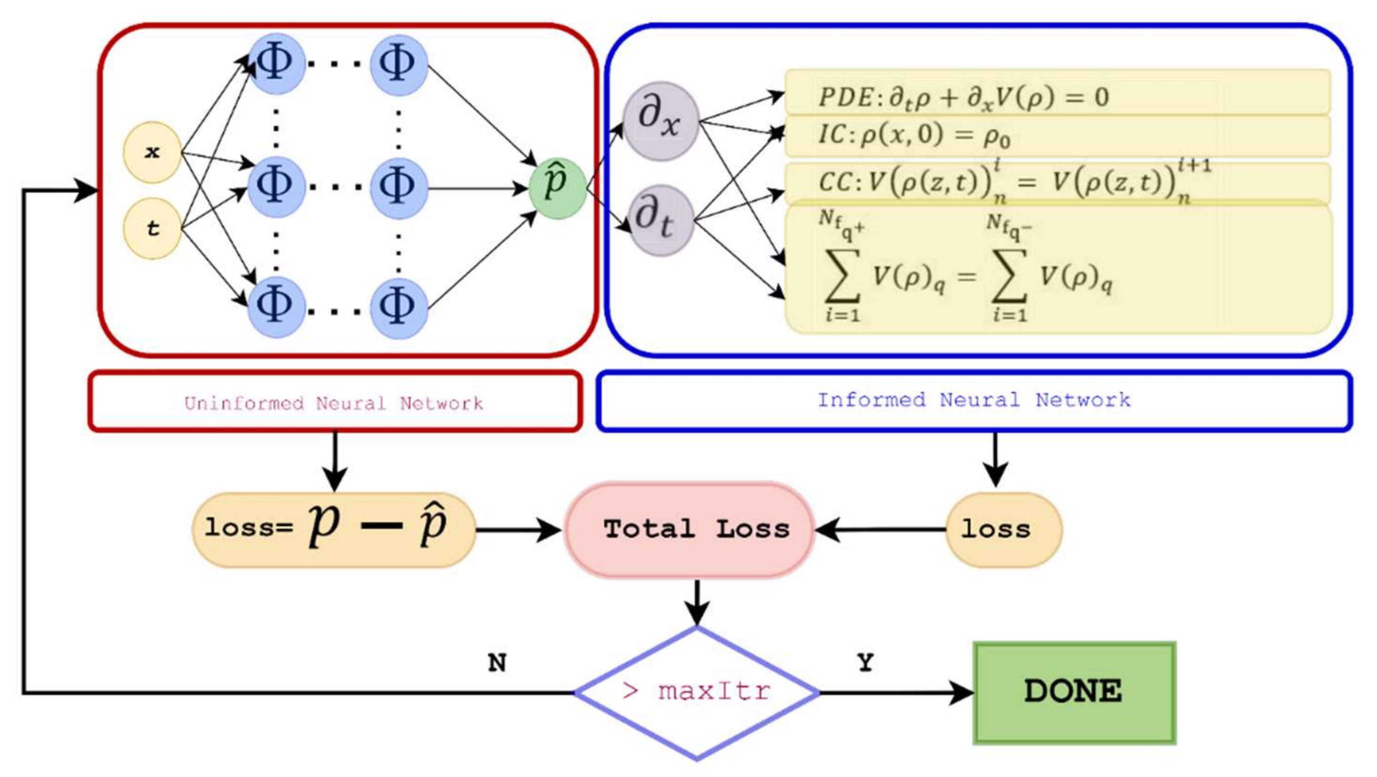
Figure 1 presents the architecture of the PINN Link-Net. The proposed framework consists of parts, i.e., physics-uninformed neural network (PUNN) and physics-informed neural network (PINN). The PUNN and PINN parts are described in detail in the following subsections.

3.1. PUNN

The physics-uninformed neural network corresponds to purely the data part. The growing amount of scientific data and rapid advances in machine learning have made data-driven approaches increasingly popular. Instead of using an existing theory, a machine learning algorithm can be employed to analyze a complex problem based solely on data. The scientific challenge is to find a model that can accurately predict new experimental measurements given existing experimental data points resulting from an unknown physical phenomenon. Input data points can be used to train neural networks, which can predict the response variable based on the set of input variables. This is usually achieved by minimizing the mean-squared error between its predictions and the given training points. In the proposed framework, the data-dependent part is the physics-uninformed neural network, owing to its black-box nature and lack of understanding of the underlying physical system. Fulari et al., 2017 developed an artificial neural network (ANN) model for traffic state estimation using erroneous data [49]. He et al., 2016 estimated freeway speeds using neural network-based fusion modules designed to combine traffic information from cellular handoff probe systems and microwave sensors [50].

3.2. PINN

Many scientific fields have adopted machine learning algorithms, but do these algorithms understand the underlying physical systems they are attempting to solve? For neural network models to understand the underlying physical system, prior scientific knowledge is incorporated into the network through governing differential equations. PINN algorithms combine the contribution of the neural network with residual terms from the governing equations, which are used as penalties to constrain the space of acceptable solutions. A PINN algorithm for the LWR Model is shown in Figure 1 with the neural network along with a physics-informed component. In addition to the contribution from the neural network, the loss function is evaluated based on the residual of the governing equation. In PINN part, the loss function consists of errors from governing PDE, initial condition, and intersection conditions. The intersection conditions include the traffic flow continuity and flow conservation at the intersection points. In order to minimize the loss function, weights (w) and biases (b) are determined such that the loss function is minimized below a specified threshold or until a maximum number of iterations is reached. The following studies have focused on PINNs in transportation related studies.
Using SUMO simulated data, Agarwal and Huang validated Greenshields-based LWR models for loop detector scenarios using the PIL algorithm [29]. Based on the data collected from probe vehicles, Barreau et al. developed a PINNs model for trajectory reconstruction [30]. Shi et al. (2020) integrated second-order ARZ model for TSE by using loop detectors and probe vehicle data [31]. They also expanded their study to estimate fundamental diagrams (FDs) and determine model parameters [32].
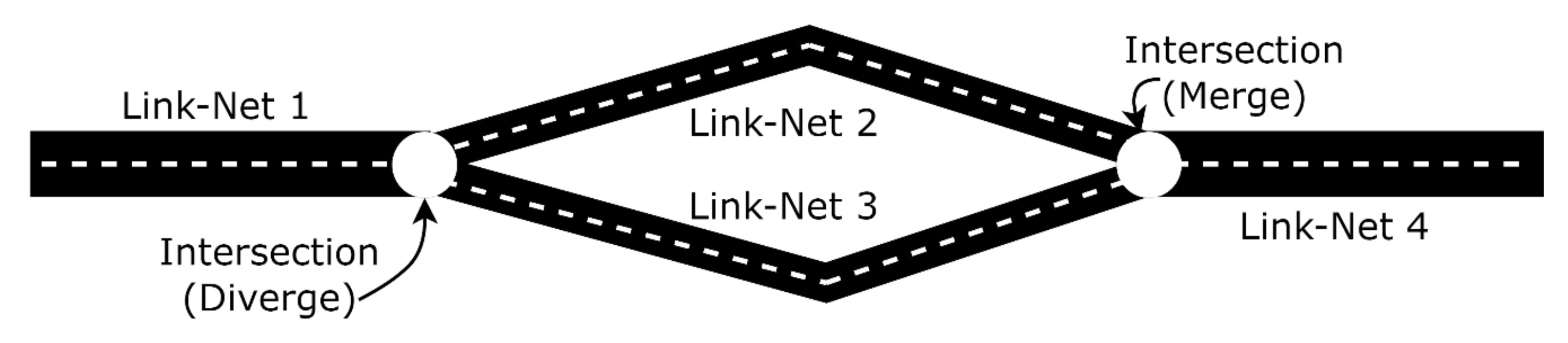
To illustrate the method in an example network, Figure 2 presents a small traffic flow network, which is composed of four links. Link-Nets are employed in each link with the different architecture of the neural networks to solve the integrated traffic flow model. The Link-Nets offer better computational efficiency through parallelization of the network. Moreover, shallow and deep networks could be employed for various links depending upon the complexity of traffic on the links.
On the traffic flow model, the general form of the partial differential equation of the Lighthill–Whitham–Richards (LWR) model of traffic flow is given by:
t ρ + x ρ v = 0 ;   v = V ρ
where ρ : ℝ + → [0, 1] is the traffic density, i.e., the number of vehicles per unit length v is the traffic speed, and V ( ρ ) is the flux which is a speed-density function.
Consider a traffic flow network consisting of N number of non-overlapping links. Let D[⋅] be a general differential operator and Ωq be a subset of the computational domain Ω. The traffic state ρ x , t at each point x , t in a continuous domain is determined such that the following traffic flow model PDE could be satisfied:
t ρ + D ρ x , t = 0 ,   x Ω q ,   t 0 , T  
The output of the PINNs for the qth link is given by
ρ θ ˜ q = N ( z ; θ ˜ q ) , z Ω q , q 1 , 2 , , N
Let { x u q i } i = 1 N u q , { x f q i } i = 1 N f q , and { x I q i } i = 1 N I q be the set of randomly drawn training, residual and intersection points in the qth link, respectively. In a qth link, the number training, residual, and intersection points are respectively represented by N u q , N f q , and N I q . On the ML part, under the PINN algorithm, the loss from PUNN and PINN for TSE is respectively given by ρ θ ˜ q and f ^ θ ˜ q . Then, a generalized form is to solve the following optimization problem:
min θ ˜ q ( θ ˜ q )
where
( θ ˜ q ) = M S E u q ( { x u q i } i = 1 N u q ; θ ˜ q ) + M S E f q ( { x f i } i = 1 N f q ; θ ˜ q )
The following flow conservation equation helps to combine the individual links and thus to find the traffic state over the entire network;
i = 1 N I q + Q q = i = 1 N I q Q q , Q q = V ( ρ )
Q represents the link flow which is a speed density function, and i, j ∈ Ω are the inward and outward traffic flow links, respectively, represented by q+ and q, at any intersection I.
Using the above set of Equation (6), the proposed neural network framework aims to predict the traffic state over the entire traffic network. The link-wise defined loss functions are extended for the whole network by connecting individual links using a connectivity matrix subject to the relevant flow continuity and conservation equations. Thus, the loss function for a qth link is given by:
( θ ˜ q ) = W u q M S E u q ( { x u q i } i = 1 N u q ; θ ˜ q ) + W f q M S E f q ( { x f q i } i = 1 N f q ; θ ˜ q ) + W I q M S E I ( { x I q i } i = 1 N I q ; θ ˜ q )
where W u q , W f q , and W I q represent the weights assigned to errors related to the training data, residual, and intersection points, respectively. At this stage, the weights are assigned manually, though they can be chosen dynamically for faster convergence, this will increase the computational load. The mean-squared errors (MSEs) are given by Equation (8).
M S E u q ( { x u q i } i = 1 N u q ; θ ˜ q ) = 1 N u q i = 1 N u q | ρ ( i ) ρ ^ ( x u q i ; θ ˜ q ) | 2 M S E f q ( { x f q i } i = 1 N f q ; θ ˜ q ) = 1 N f q i = 1 N f q | f ^ ( x f q i ; θ ˜ q ) | 2 M S E I ( { x I q i } i = 1 N f I ; θ ˜ q ) = 1 N f q [ i = 1 N I q + Q q i = 1 N I q Q q ] I
The term MSEu and MSEf are the MSE for data discrepancy (PUNN part) and physics discrepancy (PINN part) for the link q, respectively. In addition, the following flow continuity condition could be integrated into the loss function:
M S E c ( { x I c q i } i = 1 N I c q ; θ ˜ q ) = 1 N I c q i = 1 N I c q | f ^ ( x I c q i ; θ ˜ q ) N q f ^ ( x I c q i ; θ ˜ q ) 0 q + 1 | 2
The MSEc corresponds to the residual continuity condition at a common point of two connected links given by two different neural networks. The continuity condition is a special case of flow conservation where there is only one inward flow and one outward flow link. The continuity condition can be useful where the physical characteristics of the road change like the number of lanes, etc., and it is desired to split the link to separately model their traffic flow. The MSEI is the residual flux conservation condition at the intersection given by different neural networks of the links q+ and q. The superscript + over q represents the inward flow links and − over q represents the outward flow links at the intersections. The flow conservation ensures that the flow information from the incoming links is propagating to the outward flow links at the intersection. The term f ^ ( x f q i ; θ ˜ q ) represents the residual of the governing PDE of the qth link which is given by Equation (10).
f ^ ( x f q i ; θ ˜ q ) : = t ρ ^ ( x f q i ; θ ˜ q ) N [ ρ ^ ( x f q i ; θ ˜ q ) ]
We find θ ˜ q to minimize the loss function θ ˜ q for each link. A good solution can be obtained for the whole network by wisely designing the network’s architecture and providing sufficient training data points. Several optimization algorithms can be used to minimize the loss function. Stochastic gradient descent is an extensively used method. In SGD, a small set of points is randomly selected in each iteration to determine the direction of the gradient. Under the condition of single-point convexity, the SGD algorithm can avoid local minima during PUNN training. Particularly, we use the Adam optimizer, which is a version of SGD. The basic form to update the parameters in the qth link, given the initial value of parameter θ ˜ q , is given by Equation (11).
θ ˜ q ( n + 1 ) = θ ˜ q n r × ( θ ˜ q ) θ ˜ q | ( θ ˜ q = θ ˜ q n ) , q = 1 , 2 , , N
where r is the learning rate. As explained above, the traffic flux Q is described by a speed-density function with some parameters λ that best describe the data. It is difficult to obtain fine-tuned parameters, with a modest amount of data, which best explain the unknown hidden state of the system.

3.3. Activation Function (AF)

The activation function transforms the weighted summed input from the node into an output value, which is then fed to the next hidden layer or used as output. It is the activation function that decides whether or not a neuron should be activated. The activation function determines whether a neuron should be activated, i.e., whether the neuron’s input to the network is important in predicting the future. In the absence of an activation function, neurons simply perform linear transformations on inputs using weights and biases. Moreover, a neuron’s activation function adds nonlinearity to its output, enabling it to solve complex problems. Different activation functions may be used in different portions of a model, and they affect the capabilities and performances of the neural network. A neural network is usually trained with a backpropagation algorithm that requires the derivative of prediction error to update the weights of the model, which requires differentiable activation functions. There are a variety of activation functions available in the literature, including sigmoid, tanh functions, ReLUs, ELU, swish, softmax, etc. [51,52].
In addition to predefined functions, Jagtap et al. introduced adaptive activation functions by integrating a trainable hyper-parameter that accelerates PINN convergence. In their study, they showed that the adaptive activation function could be used to solve a range of forward and inverse problems more quickly and accurately [53]. For layer-wise and neuron-wise activation functions, they introduced an activation slope-based slope recovery term in the loss function to further reduce the training cost [54]. Researchers also employed physical activation functions (PAFs) derived from physical laws governing the phenomena under study [55]. They validated the performance of PAFs integrated with neurons of hidden layers in combination with other AFs by solving harmonic oscillations equation, Burger’s equation, Advection–Convection equation, etc.
Jagtap et al., 2022 proposed a Rowdy-Net with Rowdy activation functions based on Kronecker neural networks (KNNs) [56]. In KNN, Kronecker’s product made the network wide while keeping the number of trainable parameters low, thereby enabling faster convergence whereas the Rowdy activation removed the saturation zone from every layer in the network, allowing it to explore more and learn faster.
In this study, we chose the tanh activation function. In addition, we used adaptive activation, following the approach presented in [53].

4. Data

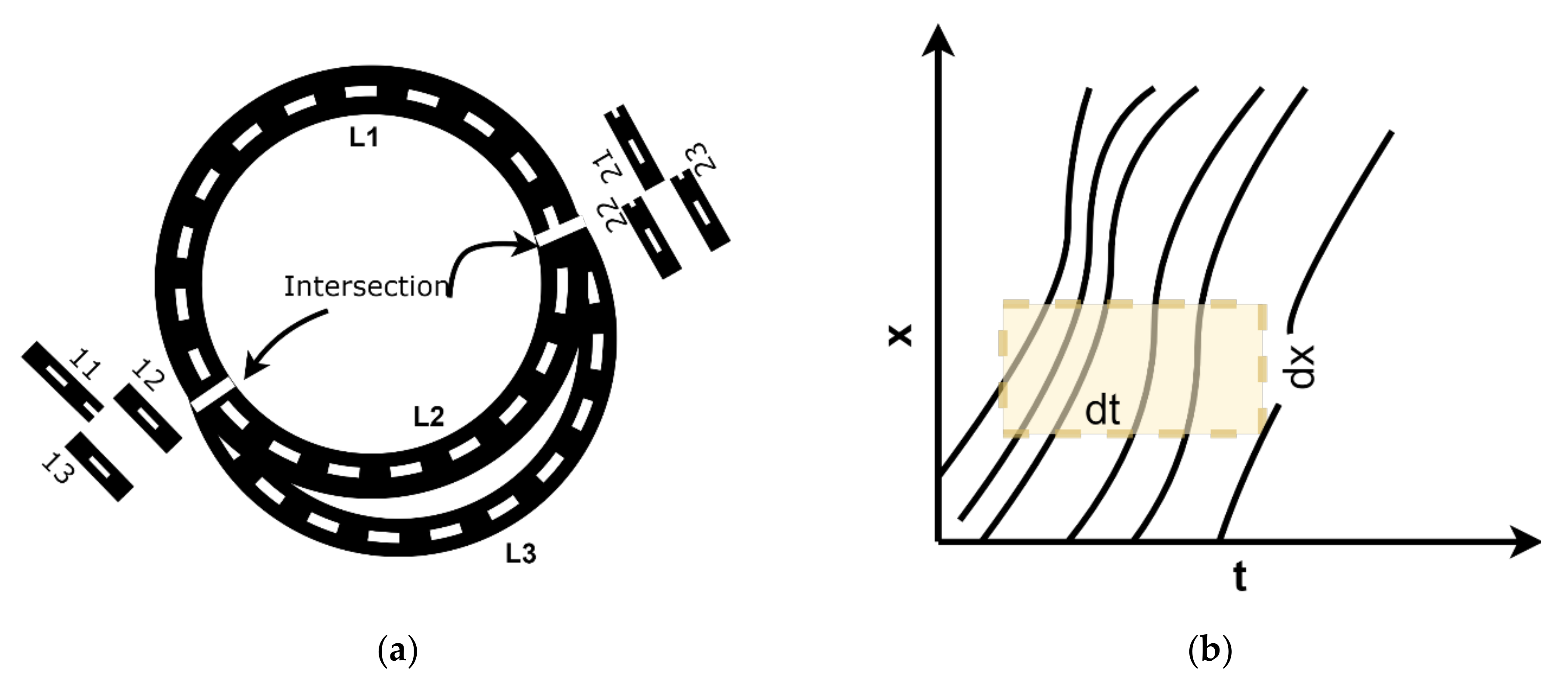
In this study, we use VISSIM simulation to generate traffic trajectory data for the circular network presented in Figure 3a, which is not on scale and it is for illustration purpose only. The traffic network consists of three links, and the length of link is set to L meters. Note that there is diverge point and a merge point in Figure 3a denoted by 1 and 2, respectively. We use connectors to join the road links in VISSIM. The traffic state data of the connectors obtained from the VISSIM were not very accurate due to the following dilemma. Connectors in VISSIM (and also in other similar simulation environments) are not dimensionless points but rather a small segment with physical length. The traffic characteristics of the short connectors are then presented by VISSIM as the average along the short distance. To achieve a higher accuracy for the average value, in theory, the connectors should be as short as possible to mimic the dimensionless points so that the data at the beginning, the ending, and throughout a short segment should be the same or very close to that. On the other hand, if segments in the simulation are too short, it may lead to computational issues such as frequent zero volume and missing observation regarding speed and density. Such a dilemma shows that there is no easy way to get the instantaneous values of speed, density, and volume of a short connector accurately. Such challenges impact the fulfillment of flow conservation equations at the merge and diverge points. In this study, we balance such challenges by keeping the connectors to be reasonably short and then try to maintain the flow conservation by using the segment data of the links at their beginnings and endings.
The traffic flows are assigned to the starting points of links L1, L2, and L3, and the traffic is let to run in the network. The obtained vehicles’ trajectory data are used to estimate the traffic speed, density, and flow. On a stretch of road with length L and time interval T, the time-space is discretized into a uniform grid with cell size dT × dL. The discrete area to estimate the traffic states is illustrated in Figure 3b. The total number of cells in the time and space dimensions are NT and NL, respectively.

4.1. Speed

The speed is assumed a constant in each cell, which is the average slope of spatiotemporal trajectories in that cell. For cells where no trajectory is detected, the speed of the adjacent cell is used to replace missing values. The average speed of cell i, j is denoted by vij where i = 1… NT, j = 1 … NL and is given by Equation (12).
v i j = 1 N v v = 1 N v Δ L v Δ T v i j
ΔLv is the distance l traveled by any vehicle v in time ΔT, and speed is stored in a matrix V ∈ R + (NT × NL).

4.2. Density

The average traffic density ρij of a cell in a time-space diagram is evaluated by
ρ i j = 1 Δ A i j   v = 1 N v Δ T v
ΔT is the total time traveled by all vehicles in a certain cell and ΔAij = dL × dT is the area of the cell.

4.3. Flow

The average traffic flow Qij of a cell in a time-space diagram is evaluated by:
Q i j = 1 Δ A i j v = 1 N v Δ L v
ΔL is the total distance traveled by all vehicles in a certain cell and ΔAij = dL × dT is the area of the cell.

5. Experimental Setup and Discussion

In this section, we test the performance of the proposed framework to estimate traffic dynamics in a traffic network based on the LWR model. Traffic data are obtained from the circular traffic network shown in Figure 3 using PTV VISSIM. The length of each link is set to 15,015 m.
In this study, we use synthetic demand to simulate the traffic in VISSIM. The traffic input flows are randomly assigned, for the initial 900 s of a simulation run, to the starting points of Links L1, L2 and L3 are 3000, 1000, and 2000 vehicles per hour, respectively, as presented in Table 1. In addition, to generate more dynamics in traffic behavior, speed reduction areas are activated for some time during the simulation run as well as activating a stochastic behavior of the vehicles. After the initial 900 s of a simulation run, the traffic is allowed to stabilize in the network for another 300 s, and trajectory data of the following 800 s are used in this study. We considered a closed traffic network in this study to observe the complete shockwave and congestion spillover in the network.
To estimate the macroscopic traffic flow parameters, the cell size in the time-space diagram is set to 5 s along the time dimension, and 5 m along the space dimension. Thus, the size of the obtained uniform grid is 160 × 3003. Five seconds is a common time step length for realistic speed data. For instance, we have real world speed data every five seconds for the major freeways from Alabama Department of Transportation. Some widely used datasets such as PeMS in California also provide speed data every five second. Therefore, we choose 5 s as ΔT. The segment length is on trial basis. It is not too short to have the frequent empty cells with no detected vehicles. It is not too long to have significant heterogeneity on traffic states within each road segment.
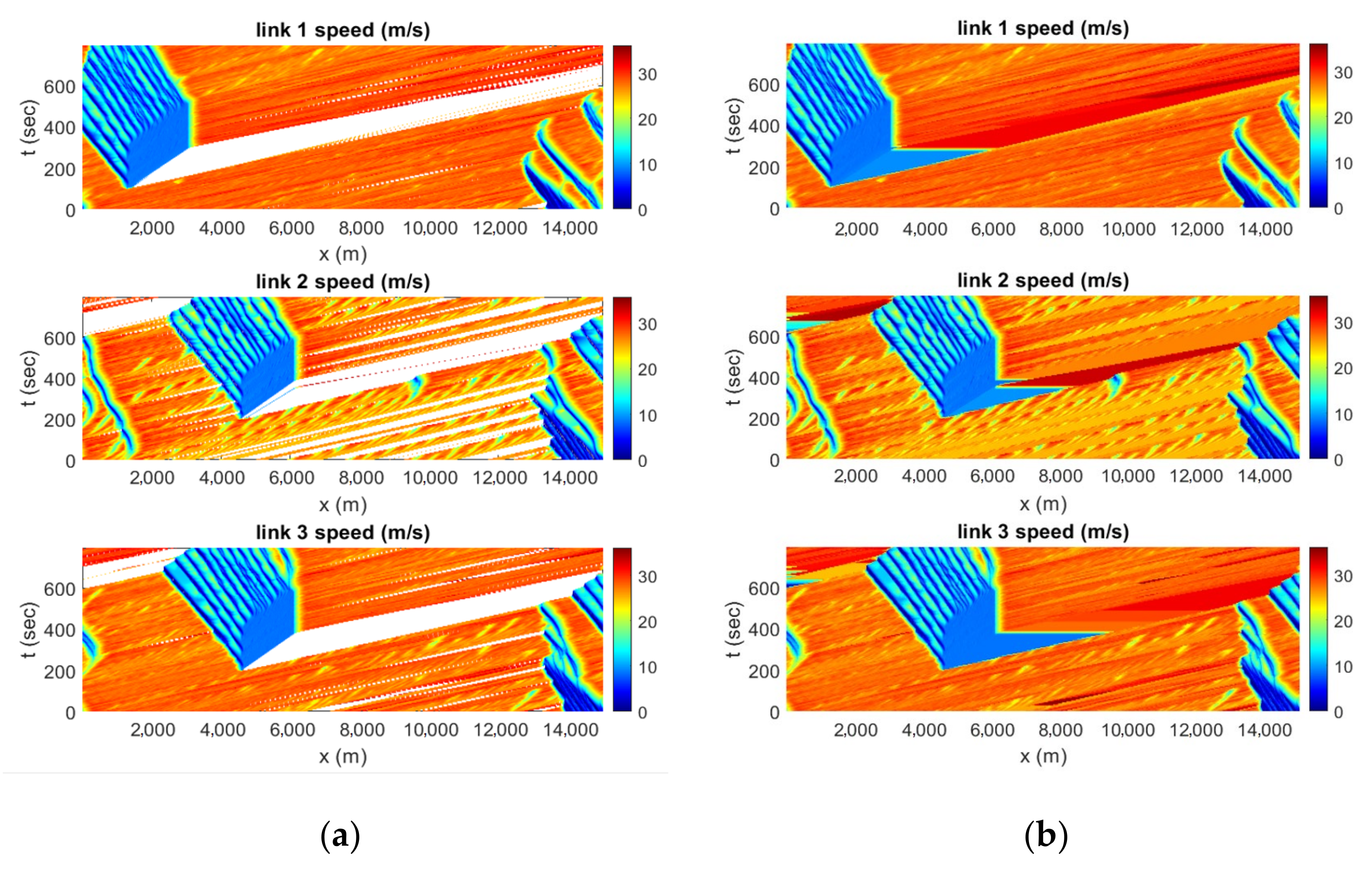
In the obtained data, there are cells, named empty cells, where the vehicles are not detected. The flow and density in the empty cells are zero, but the speed should be either close to free flow or the average speed of nearby cells. For simplicity, the speed in the empty cells is set to constant between two cells. The speed contour plot of all three links before and after filling the empty cells is presented in Figure 4a,b, respectively.
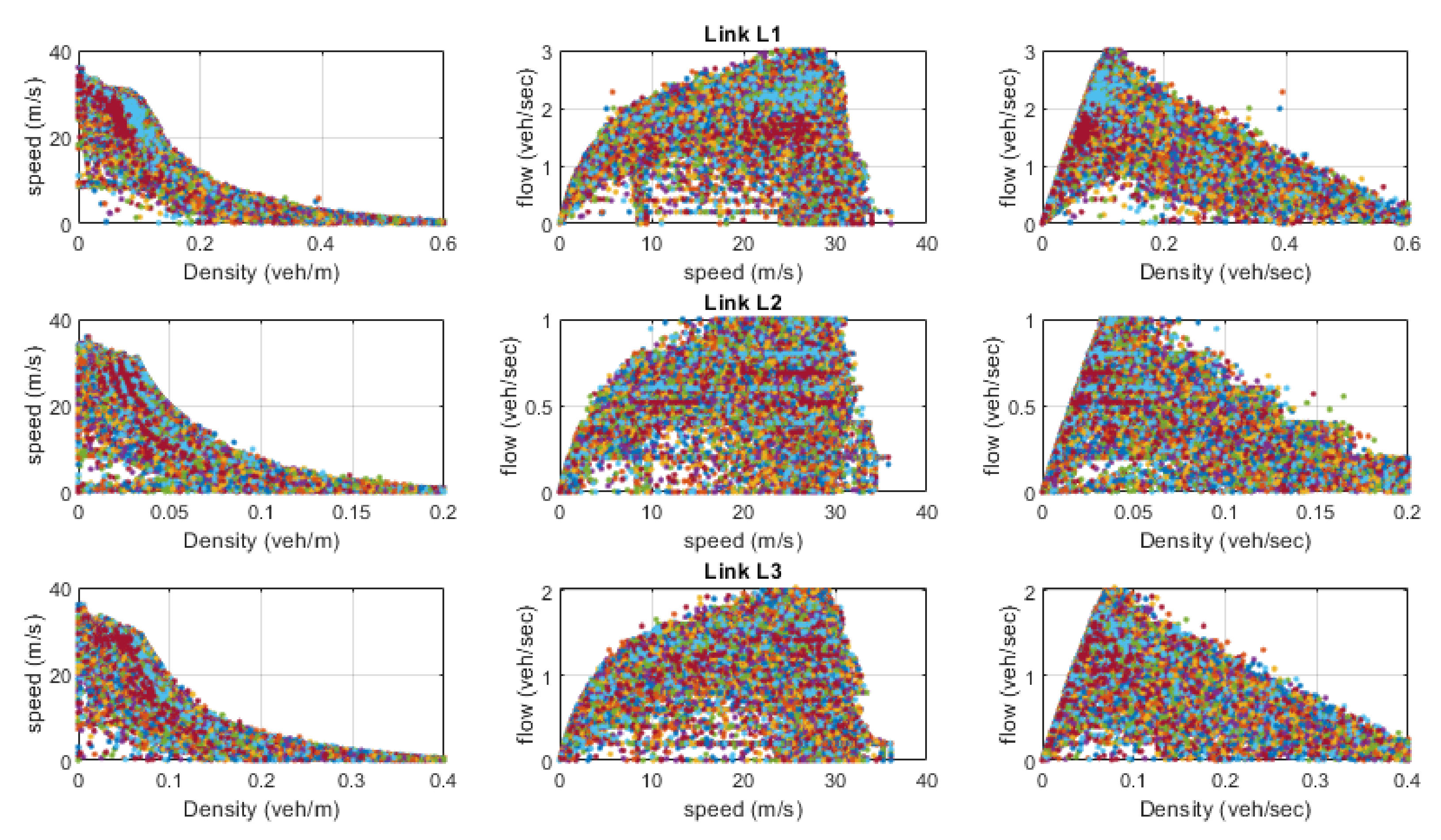
The speed, density, and flow data of the network are explored in Figure 5. The figure shows that flow-density-speed follows a similar pattern; however, the jam density and peak flows are different in various links of the network. Therefore, we left this part on the framework to estimate the best-fit parameters. The LWR model is given by t   ρ + x   V ρ = 0 . The flux function V = ρv is described as a speed-density function, and density can also be described as a function of velocity. Figure 5 shows a nonlinear relationship between speed and density. However, we consider a linear relationship following Greenshield’s Model, i.e., ρ = λ1 v + λ2. The flux function is given by V(v) = v(λ1 v + λ2), and the resulting LWR model would be λ2⋅vx + 2⋅λ1⋅v⋅vx + λ1⋅vt = 0, where λ1 and λ2 are the parameters that define the nature of the relationship between traffic state variables, and these parameters are trained during the training of the neural network.
The individual links are stitched together based on the connectivity matrix in Table 2. Each row (sub vector) in the matrix represents one link. The first, second, and third elements of a row denote link ID, start point, and end point, respectively. Node 1 or intersection 1 is the diverge point where traffic from link L1 diverges to links L2 and L3. Similarly, Node 2 is a merging point in the network where traffic from links L2 and L3 merges onto L1.
To train the proposed model, 1200 data points are randomly selected from each link of the network. There are 10 layers and 30 neurons in each layer in PINNs architecture and the input training and residual data points are 1200 and 30,000, respectively. The input data show that the model is trained using only about 0.25% of the total data points in the network.
Accuracy and performance are greatly influenced by the framework’s width, depth, and learning rate. In line with the literature, 8 hidden layers are selected for the network and a sensitivity analysis is performed to determine its width and learning rate. Learning rate is crucial when seeking global minima. The studies showed that the computational cost of a small learning rate can increase even though it moves towards global minima gradually, whereas a large learning rate can skip the global minima altogether [53]. A sensitivity analysis is presented in Table 3, which compares the relative errors of the various links for the fixed tanh activation function. A model with 8 hidden layers and 30 neurons performs the best with a learning rate of 0.001. Keeping in view the optimal parameters, the PINNs architecture and the input data points are summarized in Table 4. There are 10 layers, including an input layer, 8 hidden layers, and 1 output layer.
Keeping in view Figure 3 from the previous section, the conservation conditions Q11 = Q12 + Q13 and Q21 = Q22 + Q23 are integrated into the model for diverging and merging points, respectively. Q represents the flow V and the first and second digits in subscript refer to node and link, respectively.
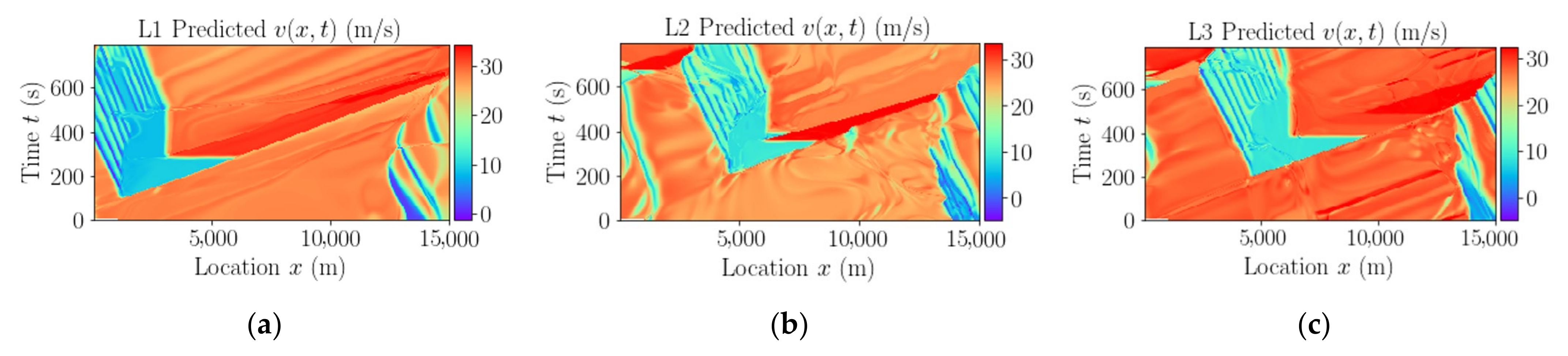
After training the model, the complete dataset of the network is passed to the model to estimate the traffic state. The predicted speeds for the links L1, L2, and L3 are respectively reported in Figure 6a–c. The predicted speed contours for all the links of the network are pretty similar to the actual speed contours counterparts in 
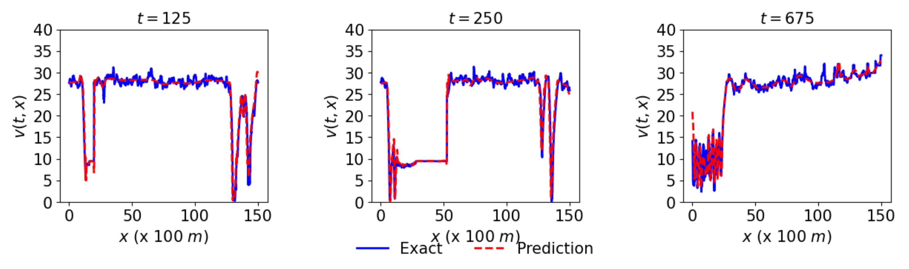
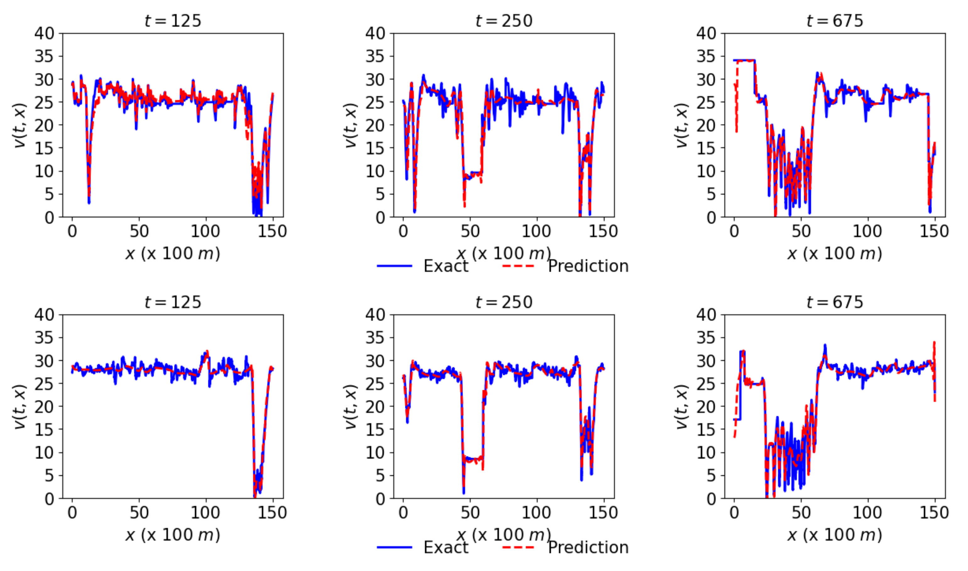
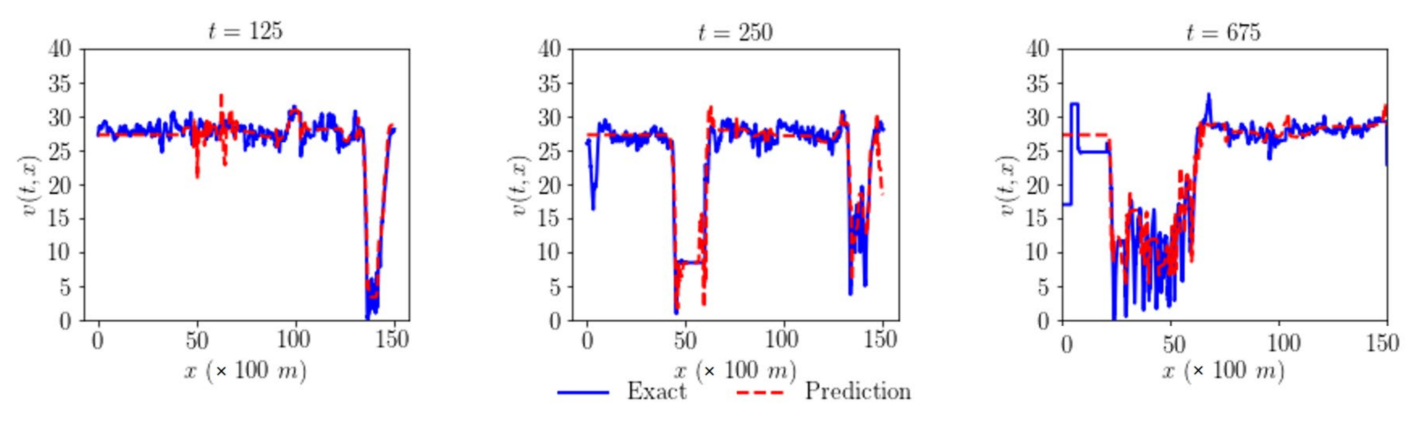
Figure 4b. The model has successfully captured the traffic dynamics of the network. The predicted data are further compared at different fixed locations along time and space dimensions. 
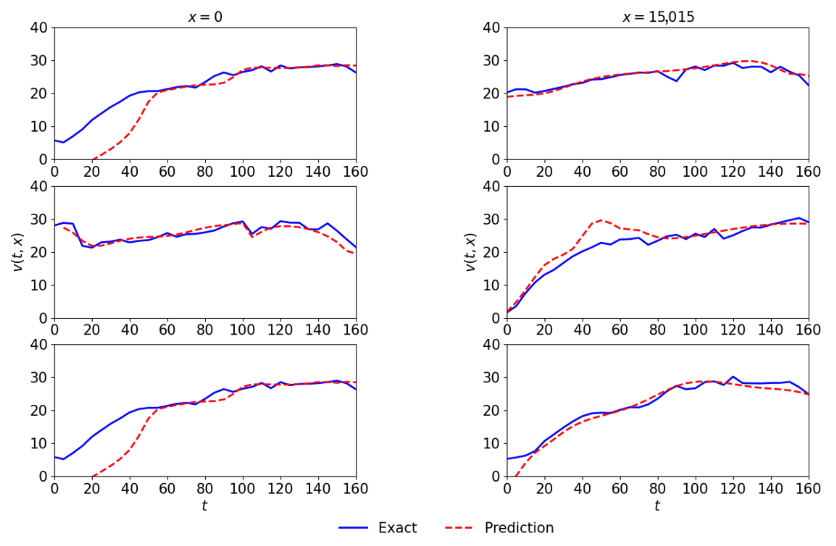
Figure 7 presents actual and predicted speed at three different times 125, 250, and 675 respectively given by the first, second, and third columns. The first, second, and third rows respectively represent the network’s links, L1, L2, and L3, that show the promising results.
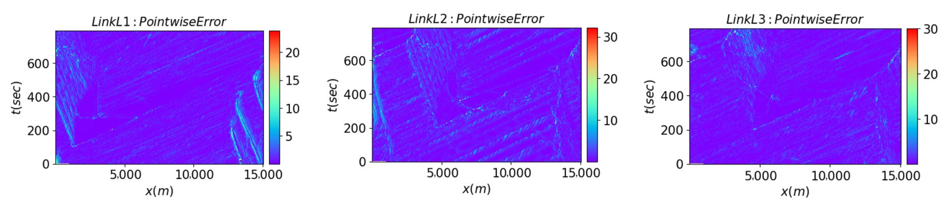
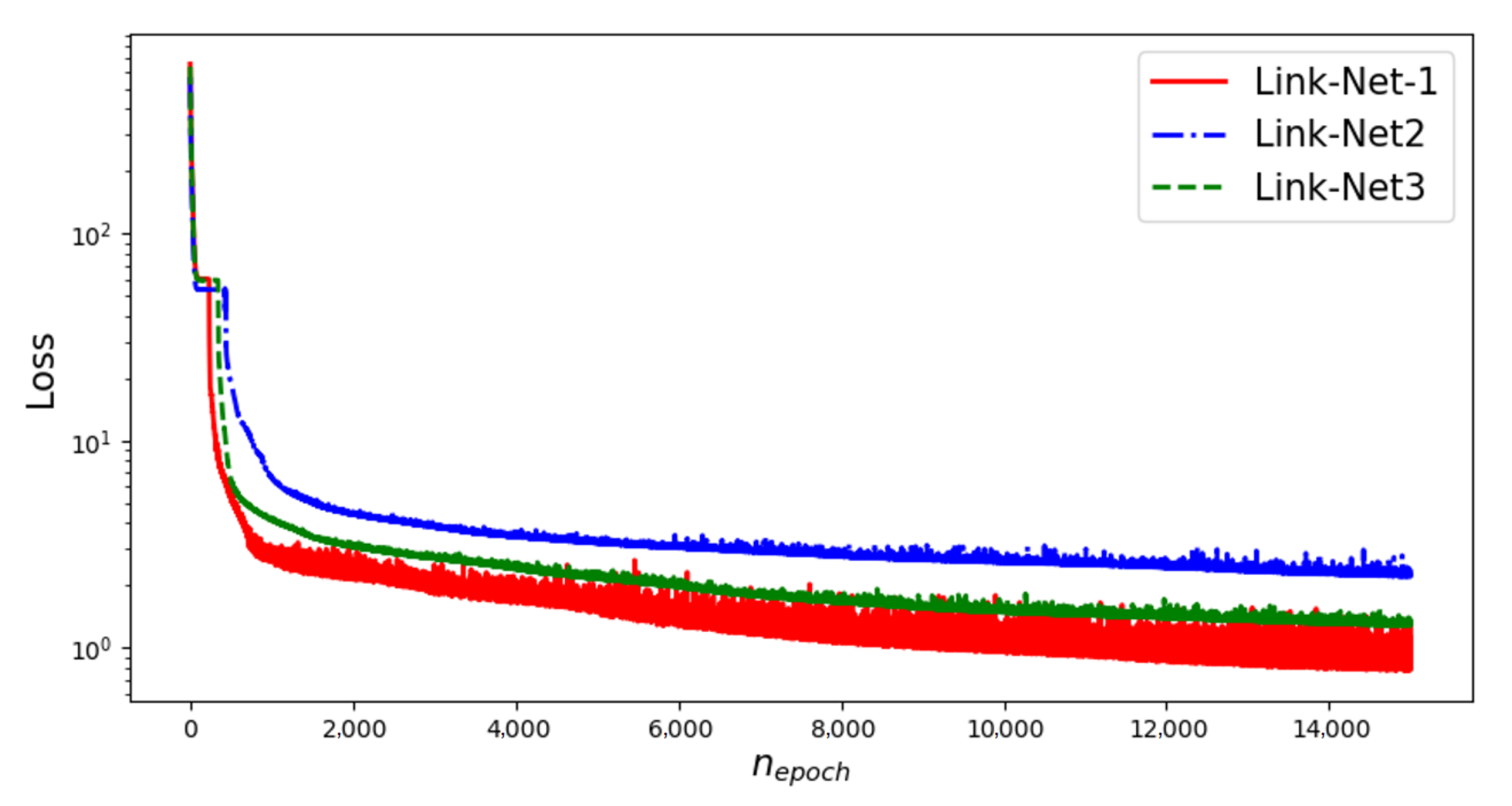
The pointwise error of all three links and the loss convergence history are presented in Figure 8 and Figure 9, respectively. Based on Figure 8, the dominant blue color indicates lower prediction error, which indicates the model effectively captures the general congestion pattern. It is evident from Figure 9 that even after 15,000 epochs, the loss for all three links remains continuously decreasing.
In our case, we use an adaptive activation function in accordance with Jagtap et al. [
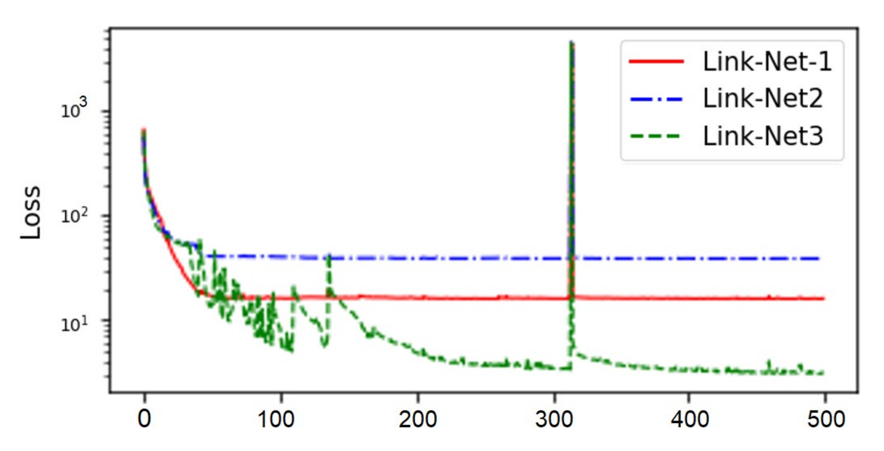
53]. However, the adaptive activation function does not significantly improve the results. Figure 10 and Figure 11 present representative results of the framework with adaptive activation. In Figure 11, the loss of links L1 and L2 does not diminish after about 50 epochs, despite a rapid convergence at the initial epochs.
Although the proposed approach successfully captured the complex traffic behavior in the network, the model needs further improvements and fine tuning to eliminate the large errors. In addition, the lesser accuracy is likely due to ambiguities in the data collection process. For example, the assumption of constant traffic state across a cell may be reasonable from a macroscopic perspective, but it may not necessarily satisfy the partial differential equation that describes traffic flow. Moreover, the data failed to follow the basic flow conservation phenomenon at the intersecting points. We further compare the data and model predictions at the intersection using Figure 12.
The larger error at the intersection points is due to discrepancies in the actual data. Since the data are estimated as described in the previous section and the data are not preprocessed to strictly satisfy the flow conservation at the intersection points. 
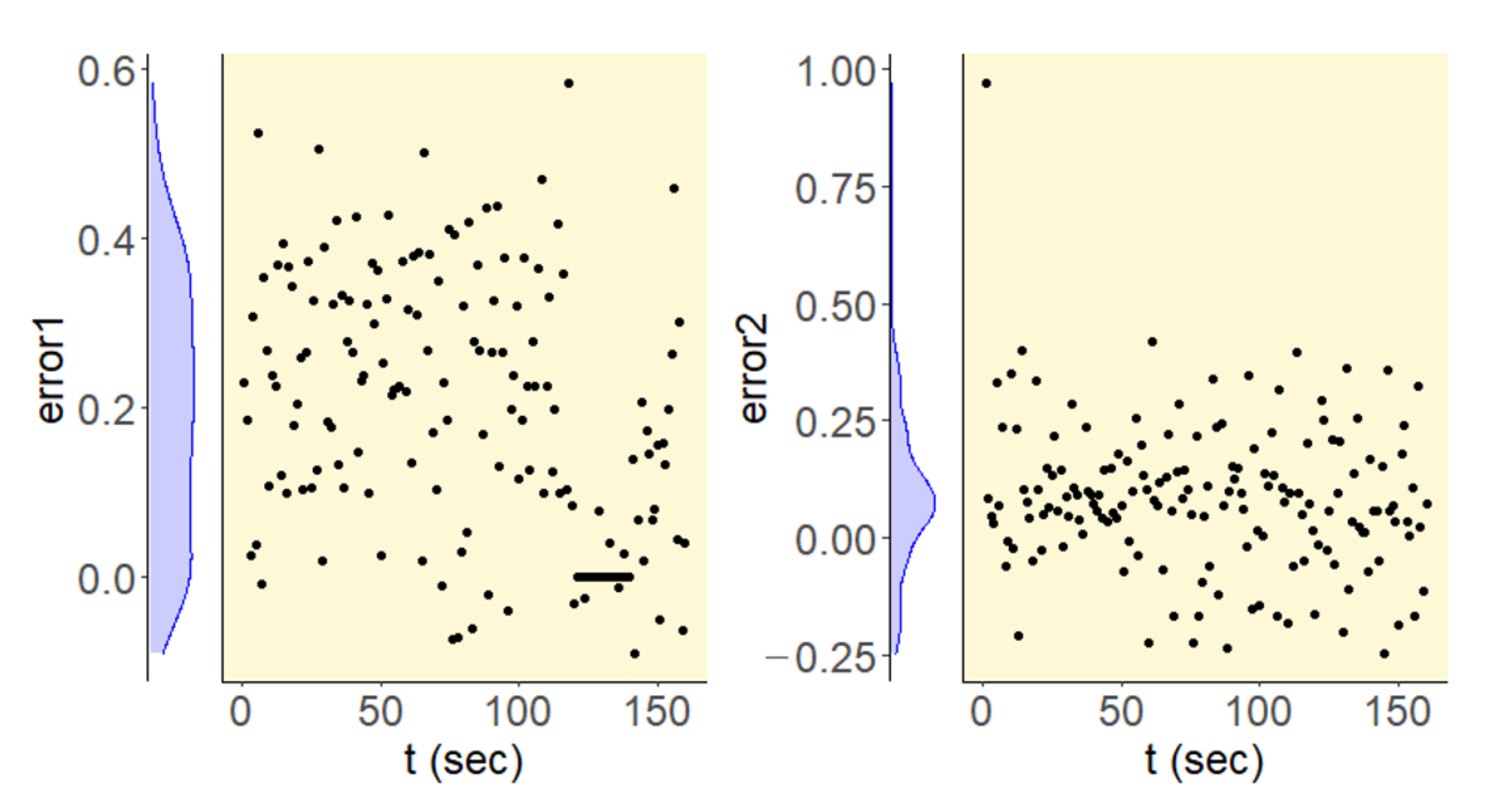
Figure 13 shows the flow conservation error1 and error2 at intersections 1 and 2, respectively. The flow conservation error in the observed data is due to the assumption of grid cells while estimating the traffic state variables from the trajectory data. The error could be reduced to zero by assuming a minimally small-sized cell. The time complexity of the algorithm to compute traffic state variables from the space-time diagram is O(n2), and a too small-sized cell could be computationally expensive. The flow conservation error distribution shows lesser violations at intersection 2 and that the prediction results are better as compared to intersection 1.

6. Conclusions

In this paper, we presented a physics-informed neural networks (PINNs) framework for traffic state estimation (TSE) in a traffic network. The study demonstrates that PINNs have the potential of utilizing extremely sparse traffic data and utilizing deep learning techniques for TSE in high accuracy using an integrated traffic flow model. A domain-decomposition approach is employed in the framework which is very useful to model characteristics of individual links in the network and change the structural complexity of the neural network of the individual links to facilitate the training process.
The experimental results show that the presented framework accurately learns the complex traffic dynamics over a circular traffic network. The predicted speeds match the actual speeds at almost all the locations other than the intersection points. The error at the intersection points is due to discrepancies in the actual data. Theoretically, the flow conservation condition must be satisfied at the intersection points. However, the actual simulated data violate the flow conservation, and this violation is potentially the result of considering average speeds over small cells. The performance of the network could be improved by refining the data through a tradeoff between the space–time diagram cell size and the computational time and improving the hyper-parameters of the neural network in future research. Moreover, equal weights are applied to various errors in the cumulative loss function while training the model, which may be tuned up in the future research to achieve better performances. The application of the proposed framework can be expanded to large-scale networks with data fusion from multiple sources in future research and practices.

Author Contributions

The authors confirm contribution to the paper as follows: study conception and design: R.M. and M.U.; data preparation: M.W. and J.H.; analysis and interpretation of results: R.M. and M.U.; draft manuscript preparation: R.M. and M.U. All authors have read and agreed to the published version of the manuscript.

Funding

This research received no external funding.

Conflicts of Interest

The authors declare no conflict of interest.

References

  1. Treiber, M.; Kesting, A.; Wilson, R.E. Reconstructing the traffic state by fusion of heterogeneous data. Comput.-Aided Civ. Infrastruct. Eng. 2010, 26, 408–419. [Google Scholar] [CrossRef] [Green Version]
  2. Bekiaris-Liberis, N.; Roncoli, C.; Papageorgiou, M. Highway traffic state estimation with mixed connected and conventional vehicles. IEEE Trans. Intell. Transp. Syst. 2016, 17, 3484–3497. [Google Scholar] [CrossRef] [Green Version]
  3. Agarwal, S.; Kachroo, P.; Contreras, S. A Dynamic Network Modeling-based approach for traffic observability problem. IEEE Trans. Intell. Transp. Syst. 2016, 17, 1168–1178. [Google Scholar] [CrossRef]
  4. Seo, T.; Bayen, A.M.; Kusakabe, T.; Asakura, Y. Traffic State Estimation on Highway: A Comprehensive Survey. Annu. Rev. Control 2017, 43, 128–151. [Google Scholar] [CrossRef] [Green Version]
  5. Lighthill, M.J.; Whitham, G.B. On Kinematic Waves II. A theory of traffic flow on long crowded roads. Proc. R. Soc. Lond. Ser. A. Math. Phys. Sci. 1955, 229, 317–345. [Google Scholar] [CrossRef]
  6. Richards, P.I. Shock waves on the highway. Oper. Res. 1956, 4, 42–51. [Google Scholar] [CrossRef]
  7. Yuan, Y.; Zhang, Z.; Yang, X.T.; Zhe, S. Macroscopic traffic flow modeling with physics regularized gaussian process: A new insight into machine learning applications in transportation. Transp. Res. Part B Methodol. 2021, 146, 88–110. [Google Scholar] [CrossRef]
  8. Raissi, M.; Karniadakis, G.E. Hidden physics models: Machine learning of nonlinear partial differential equations. J. Comput. Phys. 2018, 357, 125–141. [Google Scholar] [CrossRef] [Green Version]
  9. Jagtap, A.D.; Karniadakis, G.E. Extended physics-informed Neural Networks (xpinns): A generalized space-time domain decomposition based deep learning framework for nonlinear partial differential equations. Commun. Comput. Phys. 2020, 28, 2002–2041. [Google Scholar] [CrossRef]
  10. Flynn, M.R.; Kasimov, A.R.; Nave, J.C.; Rosales, R.R.; Seibold, B. Self-sustained nonlinear waves in traffic flow. Phys. Rev. E 2009, 79, 056113. [Google Scholar] [CrossRef]
  11. Payne, H.J. Models of Freeway Traffic and Control. In Mathematical Models of Public Systems; Simulation Councils: Huntsville, AL, USA, 1971; Volume 1, pp. 51–61. [Google Scholar]
  12. Aw, A.; Rascle, M. Resurrection of “second order” models of Traffic Flow. SIAM J. Appl. Math. 2000, 60, 916–938. [Google Scholar] [CrossRef] [Green Version]
  13. Zhang, H.M. A non-equilibrium traffic model devoid of gas-like behavior. Transp. Res. Part B Methodol. 2002, 36, 275–290. [Google Scholar] [CrossRef]
  14. Smith, B.L.; Scherer, W.T.; Conklin, J.H. Exploring imputation techniques for missing data in Transportation Management Systems. Transp. Res. Rec. J. Transp. Res. Board 2003, 1836, 132–142. [Google Scholar] [CrossRef]
  15. Chen, C.; Kwon, J.; Rice, J.; Skabardonis, A.; Varaiya, P. Detecting errors and imputing missing data for single-loop surveillance systems. Transp. Res. Rec. J. Transp. Res. Board 2003, 1855, 160–167. [Google Scholar] [CrossRef]
  16. Zhong, M.; Lingras, P.; Sharma, S. Estimation of missing traffic counts using factor, genetic, neural, and regression techniques. Transp. Res. Part C Emerg. Technol. 2004, 12, 139–166. [Google Scholar] [CrossRef]
  17. Ni, D.; Leonard, J.D. Markov chain Monte Carlo multiple imputation using Bayesian networks for Incomplete Intelligent Transportation Systems Data. Transp. Res. Rec. J. Transp. Res. Board 2005, 1935, 57–67. [Google Scholar] [CrossRef]
  18. Tan, H.; Wu, Y.; Cheng, B.; Wang, W.; Ran, B. Robust missing traffic flow imputation considering nonnegativity and road capacity. Math. Probl. Eng. 2014, 2014, 763469. [Google Scholar] [CrossRef] [Green Version]
  19. Tan, H.; Feng, G.; Feng, J.; Wang, W.; Zhang, Y.-J.; Li, F. A tensor-based method for missing traffic data completion. Transp. Res. Part C Emerg. Technol. 2013, 28, 15–27. [Google Scholar] [CrossRef] [Green Version]
  20. Polson, N.G.; Sokolov, V.O. Deep learning for short-term traffic flow prediction. Transp. Res. Part C Emerg. Technol. 2017, 79, 1–17. [Google Scholar] [CrossRef] [Green Version]
  21. Chen, Y.; Chen, X.M. A novel reinforced dynamic graph convolutional network model with data imputation for network-wide traffic flow prediction. Transp. Res. Part C Emerg. Technol. 2022, 143, 103820. [Google Scholar] [CrossRef]
  22. Xu, D.; Peng, H.; Wei, C.; Shang, X.; Li, H. Traffic State data imputation: An efficient generating method based on the graph aggregator. IEEE Trans. Intell. Transp. Syst. 2022, 23, 13084–13093. [Google Scholar] [CrossRef]
  23. Zhang, T.; Guo, G. Graph attention LSTM: A spatiotemporal approach for traffic flow forecasting. IEEE Intell. Transp. Syst. Mag. 2022, 14, 190–196. [Google Scholar] [CrossRef]
  24. Rempe, F.; Franeck, P.; Bogenberger, K. On the estimation of traffic speeds with deep convolutional neural networks given probe data. Transp. Res. Part C Emerg. Technol. 2022, 134, 103448. [Google Scholar] [CrossRef]
  25. Zhang, Z.; Lin, X.; Li, M.; Wang, Y. A customized deep learning approach to integrate network-scale online traffic data imputation and prediction. Transp. Res. Part C Emerg. Technol. 2021, 132, 103372. [Google Scholar] [CrossRef]
  26. Ye, Y.; Zhang, S.; Yu, J.J.Q. Traffic data imputation with ensemble convolutional Autoencoder. In Proceedings of the 2021 IEEE International Intelligent Transportation Systems Conference (ITSC), Indianapolis, IN, USA, 19–22 September 2021. [Google Scholar]
  27. Duan, Y.; Lv, Y.; Liu, Y.-L.; Wang, F.-Y. An efficient realization of deep learning for traffic data imputation. Transp. Res. Part C Emerg. Technol. 2016, 72, 168–181. [Google Scholar] [CrossRef]
  28. Liang, Y.; Zhao, Z.; Sun, L. Memory-augmented dynamic graph convolution networks for traffic data imputation with diverse missing patterns. Transp. Res. Part C Emerg. Technol. 2022, 143, 103826. [Google Scholar] [CrossRef]
  29. Huang, A.J.; Agarwal, S. Physics informed Deep Learning for traffic state estimation. In Proceedings of the 2020 IEEE 23rd International Conference on Intelligent Transportation Systems (ITSC), Rhodes, Greece, 20–23 September 2020. [Google Scholar] [CrossRef]
  30. Barreau, M.; Aguiar, M.; Liu, J.; Johansson, K.H. Physics-informed learning for identification and state reconstruction of traffic density. In Proceedings of the 2021 60th IEEE Conference on Decision and Control (CDC), Austin, TX, USA, 13–17 December 2021. [Google Scholar] [CrossRef]
  31. Shi, R.; Mo, Z.; Di, X. Physics-Informed Deep Learning for Traffic State Estimation: A Hybrid Paradigm Informed by Second-Order Traffic Models. In Proceedings of the AAAI Conference on Artificial Intelligence, Online, 2–9 February 2021; Volume 35, pp. 540–547. [Google Scholar]
  32. Shi, R.; Mo, Z.; Huang, K.; Di, X.; Du, Q. A Physics-Informed Deep Learning Paradigm for Traffic State and Fundamental Diagram Estimation. IEEE Trans. Intell. Transp. Syst. 2022, 23, 11688–11698. [Google Scholar] [CrossRef]
  33. Thodi, B.T.; Khan, Z.S.; Jabari, S.E.; Menendez, M. Incorporating kinematic wave theory into a deep learning method for high-resolution traffic speed estimation. IEEE Trans. Intell. Transp. Syst. 2022, 23, 17849–17862. [Google Scholar] [CrossRef]
  34. Owhadi, H. Bayesian numerical homogenization. Multiscale Modeling Simul. 2015, 13, 812–828. [Google Scholar] [CrossRef] [Green Version]
  35. Raissi, M.; Perdikaris, P.; Karniadakis, G.E. Inferring solutions of differential equations using noisy multi-fidelity data. J. Comput. Phys. 2017, 335, 736–746. [Google Scholar] [CrossRef] [Green Version]
  36. Pang, G.; Lu, L.; Karniadakis, G.E. FPINNs: Fractional physics-informed Neural Networks. SIAM J. Sci. Comput. 2019, 41, A2603–A2626. [Google Scholar] [CrossRef] [Green Version]
  37. Zhang, D.; Guo, L.; Karniadakis, G.E. Learning in modal space: Solving time-dependent stochastic pdes using physics-informed Neural Networks. SIAM J. Sci. Comput. 2020, 42, A639–A665. [Google Scholar] [CrossRef]
  38. Kharazmi, E.; Zhang, Z.; Karniadakis, G.E.M. HP-VPINNs: Variational physics-informed neural networks with domain decomposition. Comput. Methods Appl. Mech. Eng. 2021, 374, 113547. [Google Scholar] [CrossRef]
  39. Shukla, K.; Jagtap, A.D.; Blackshire, J.L.; Sparkman, D.; Em Karniadakis, G. A physics-informed neural network for quantifying the microstructural properties of polycrystalline nickel using ultrasound data: A promising approach for solving inverse problems. IEEE Signal Processing Mag. 2022, 39, 68–77. [Google Scholar] [CrossRef]
  40. Jagtap, A.D.; Mitsotakis, D.; Karniadakis, G.E. Deep learning of inverse water waves problems using multi-fidelity data: Application to serre–green–naghdi equations. Ocean Eng. 2022, 248, 110775. [Google Scholar] [CrossRef]
  41. McClenny, L.; Braga-Neto, U. Self-Adaptive Physics-Informed Neural Networks using a Soft Attention Mechanism. arXiv 2020, arXiv:2009.04544. [Google Scholar]
  42. Mao, Z.; Jagtap, A.D.; Karniadakis, G.E. Physics-informed neural networks for high-speed flows. Comput. Methods Appl. Mech. Eng. 2020, 360, 112789. [Google Scholar] [CrossRef]
  43. Jagtap, A.D.; Kharazmi, E.; Karniadakis, G.E. Conservative physics-informed neural networks on discrete domains for conservation laws: Applications to forward and inverse problems. Comput. Methods Appl. Mech. Eng. 2020, 365, 113028. [Google Scholar] [CrossRef]
  44. Shukla, K.; Jagtap, A.D.; Karniadakis, G.E. Parallel physics-informed neural networks via domain decomposition. J. Comput. Phys. 2021, 447, 110683. [Google Scholar] [CrossRef]
  45. Jagtap, A.D.; Mao, Z.; Adams, N.; Karniadakis, G.E. Physics-informed neural networks for inverse problems in supersonic flows. J. Comput. Phys. 2022, 466, 111402. [Google Scholar] [CrossRef]
  46. Mishra, S.; Molinaro, R. Estimates on the generalization error of physics-informed neural networks for approximating a class of inverse problems for pdes. IMA J. Numer. Anal. 2021, 42, 981–1022. [Google Scholar] [CrossRef]
  47. Ryck, T.D.; Jagtap, A.D.; Mishra, S. Error estimates for physics informed neural networks approximating the Navier-Stokes equations. arXiv 2022, arXiv:2203.09346. [Google Scholar]
  48. Hu, Z.; Jagtap, A.D.; Karniadakis, G.E.; Kawaguchi, K. When do extended physics-informed Neural Networks (xpinns) improve generalization? SIAM J. Sci. Comput. 2022, 44, A3158–A3182. [Google Scholar] [CrossRef]
  49. Fulari, S.; Vanajakshi, L.; Subramanian, S.C. Artificial Neural Network–based traffic state estimation using Erroneous Automated Sensor Data. J. Transp. Eng. Part A Syst. 2017, 143, 05017003. [Google Scholar] [CrossRef]
  50. He, S.; Zhang, J.; Cheng, Y.; Wan, X.; Ran, B. Freeway multisensor data fusion approach integrating data from cellphone probes and fixed sensors. J. Sens. 2016, 2016, 7269382. [Google Scholar] [CrossRef] [Green Version]
  51. Apicella, A.; Donnarumma, F.; Isgrò, F.; Prevete, R. A survey on modern trainable activation functions. Neural Netw. 2021, 138, 14–32. [Google Scholar] [CrossRef] [PubMed]
  52. Jagtap, A.D.; Karniadakis, G.E. How important are activation functions in regression and classification? A survey, performance comparison, and future directions. arXiv 2022, arXiv:2209.02681. [Google Scholar]
  53. Jagtap, A.D.; Kawaguchi, K.; Karniadakis, G.E. Adaptive activation functions accelerate convergence in deep and physics-informed Neural Networks. J. Comput. Phys. 2020, 404, 109136. [Google Scholar] [CrossRef] [Green Version]
  54. Jagtap, A.D.; Kawaguchi, K.; Em Karniadakis, G. Locally adaptive activation functions with slope recovery for deep and physics-informed Neural Networks. Proc. R. Soc. A Math. Phys. Eng. Sci. 2020, 476, 20200334. [Google Scholar] [CrossRef]
  55. Abbasi, J.; Andersen, P.Ø. Physical Activation Functions (PAFs): An Approach for More Efficient Induction of Physics into Physics-Informed Neural Networks (PINNs). arXiv 2022, arXiv:2205.14630. [Google Scholar]
  56. Jagtap, A.D.; Shin, Y.; Kawaguchi, K. Deep Kronecker neural networks: A general framework for neural networks with adaptive activation functions. Neurocomputing 2022, 468, 165–180. [Google Scholar] [CrossRef]
Figure 1. Neural network architecture of the proposed algorithm.
Algorithms 15 00447 g001
Figure 2. Illustration of network, Links, and Intersections.
Algorithms 15 00447 g002
Figure 3. (a) Traffic network with three links and two intersection points; (b) the trajectories of the vehicles and a discrete area to estimate the traffic states.
Algorithms 15 00447 g003
Figure 4. (a) Speed contour plot showing cells where no vehicle detected; (b) speed contour where missing cells filled with the speed of neighboring cells.
Algorithms 15 00447 g004
Figure 5. Speed, density, and flow plot of links in the network.
Algorithms 15 00447 g005
Figure 6. (a) Predicted traffic speed of Link L1, (b) predicted traffic speed of Link L2; (c) predicted traffic speed of Link L3.
Algorithms 15 00447 g006
Figure 7. Actual and predicted speed at three different times 125, 250, and 675 respectively given by the first, second, and third columns. The first, second, and third rows respectively represent the network’s links L1, L2, and L3.
Algorithms 15 00447 g007aAlgorithms 15 00447 g007b
Figure 8. Pointwise error of Links L1, L2, and L3.
Algorithms 15 00447 g008
Figure 9. Loss history over the number of epochs with fixed tanh activation function.
Algorithms 15 00447 g009
Figure 10. Actual and predicted speed at three different time intervals of Link L3 with adaptive activation function.
Algorithms 15 00447 g010
Figure 11. Loss history of all three links for 500 epochs with adaptive activation function.
Algorithms 15 00447 g011
Figure 12. Actual and predicted speed at two intersections i.e., at x = 0 and x = 15,015 m, respectively given by the first and second columns. The first, second, and third rows respectively represent the network’s links L1, L2, and L3.
Algorithms 15 00447 g012
Figure 13. Flow conservation error in the actual data at the intersection points.
Algorithms 15 00447 g013
Table 1. Synthetic traffic demand assigned to links in the network.
LinkIntervalTraffic VolumeVolume Type
L10–9003000Stochastic
900–18000Stochastic
2700–36000Stochastic
L20–9001000Stochastic
900–18000Stochastic
1800–27000Stochastic
2700–36000Stochastic
L30–9002000Stochastic
900–18000Stochastic
1800–27000Stochastic
2700–36000Stochastic
Table 2. Links and their connectivity matrix.
LinkStart NodeEnd Node
L121
L212
L312
Table 3. Relative error of links for the fixed tanh activation function.
Learning RateLayersL1L2L3
0.00018 × [30]0.15080.16040.1302
8 × [50]0.10770.174930.1193
0.0018 × [30]0.054980.075360.05237
8 × [50]0.08490.15570.127
0.018 × [30]0.29840.30380.3044
8 × [50]0.29840.30380.3043
Table 4. PINNs architecture and summary of data points in each link of the network.
LinkL1L2L3
No. of layers101010
Neurons303030
No. of Training points120012001200
No. of Residual points30,00030,00030,000
Total points in the link480,480480,480480,480
Publisher’s Note: MDPI stays neutral with regard to jurisdictional claims in published maps and institutional affiliations.

