An Auto-Encoder with Genetic Algorithm for High Dimensional Data: Towards Accurate and Interpretable Outlier Detection

Abstract

When dealing with high-dimensional data, such as in biometric, e-commerce, or industrial applications, it is extremely hard to capture the abnormalities in full space due to the curse of dimensionality. Furthermore, it is becoming increasingly complicated but essential to provide interpretations for outlier detection results in high-dimensional space as a consequence of the large number of features. To alleviate these issues, we propose a new model based on a Variational AutoEncoder and Genetic Algorithm (VAEGA) for detecting outliers in subspaces of high-dimensional data. The proposed model employs a neural network to create a probabilistic dimensionality reduction variational autoencoder (VAE) that applies its low-dimensional hidden space to characterize the high-dimensional inputs. Then, the hidden vector is sampled randomly from the hidden space to reconstruct the data so that it closely matches the input data. The reconstruction error is then computed to determine an outlier score, and samples exceeding the threshold are tentatively identified as outliers. In the second step, a genetic algorithm (GA) is used as a basis for examining and analyzing the abnormal subspace of the outlier set obtained by the VAE layer. After encoding the outlier dataset’s subspaces, the degree of anomaly for the detected subspaces is calculated using the redefined fitness function. Finally, the abnormal subspace is calculated for the detected point by selecting the subspace with the highest degree of anomaly. The clustering of abnormal subspaces helps filter outliers that are mislabeled (false positives), and the VAE layer adjusts the network weights based on the false positives. When compared to other methods using five public datasets, the VAEGA outlier detection model results are highly interpretable and outperform or have competitive performance compared to current contemporary methods.

1. Introduction

Hawkins defined the notion of an outlier as an observation that diverges greatly from the other observations so as to trigger suspicions that it was generated by a separate mechanism [1]. Detecting outliers is the process of determining whether the data have input errors and detecting unusual patterns that are substantially different from the bulk of the data. The detection of outliers is a critical step in data analysis that needs to be prioritized with meticulous attention as data containing outliers can negatively influence the accuracy of a model [2], increase the likelihood of false positives [3], lead to wrong decisions [4], and make the model computationally costly [5]. Thus, it is imperative to pay close consideration to the outliers in the data and analyze their causes to provide opportunities to discover problems and strengthen the decision-making [6]. Outlier detection has been extensively used in a multitude of fields, such as fraud detection [7], network intrusion detection [8], medical diagnosis [9], video surveillance [10], and fault diagnosis [11] etc.

As high-dimensional data continues to grow exponentially, it enables data sharing and provides a solid basis for analysis and prediction. Nonetheless, it poses great challenges to the processing and detection of outlier detection methods. One of the most notable problems is the curse of dimensionality [12]. The large number of dimensions for high-dimensional data makes the concepts of distance and proximity calculations in high-dimensional space unreliable. Therefore, they are unsuitable to be used as an effective indicator for abnormality measurement. The sparsity between the dimensions makes almost every point depict an anomalous characteristic. In addition, it is exceedingly expensive to search through the full space of high-dimensional data to obtain abnormal subspace features. Furthermore, some existing outlier detection methods are prone to a high false positive rate. That is, the major portion of the detected outliers are not actually anomalies in the actual application domains. Finally, it is becoming increasingly complicated but essential to provide interpretations for outlier detection results in high-dimensional space as a consequence of the large number of features.

In order to improve the interpretation of high-dimensional outliers and alleviate the challenges related to high-dimensional data, we propose an unsupervised outlier detection method for high-dimensional datasets based on variational autoencoders and genetic algorithms (VAEGA). The model is divided into two parts. In the first part, we build a variational encoder and decoder layer with a neural network. This is attained by feeding normal unlabeled data as input for training and iteratively learning the best encoding–decoding strategy to effectively represent the high-dimensional data distribution. Using the probability distribution of the VAE’s hidden space, hidden vectors are randomly sampled to reconstruct the data. Next, the reconstruction error of the data is calculated, and outliers are identified among the test samples whose values transcend the model’s threshold value. Even though the variational encoder and decoder layers are capable of effectively detecting the outliers, despite the curse of dimensionality, the results are prone to false positives and lack of desired interpretability.

In order to address and propose a solution to such a defect, we apply a genetic algorithm (GA) in the second part of our model. We train the genetic algorithm (GA) layer, and it searches for the abnormal subspace of the outliers that we observed in the first part. Each subspace has a fitness function that measures the degree of abnormality of each outlier detected in that subspace. The abnormal subspace of the training dataset is utilized to effectively filter false positives. The top abnormal subspace also provides insightful and explanatory interpretations for the context where the outliers are detected.

Specifically, in this paper, the main contributions are extensions of our conference work [13], and they are summarized as follows:

• We propose a model based on variational autoencoders and genetic algorithms (VAEGA) that is designed to effectively identify high-dimensional outliers and to provide accurate interpretations of the subspaces where these outliers are located.
• We utilize a VAE to effectively compress the high-dimensional data into a hidden space. After that, the hidden vectors are decoded based on the probability distribution of the hidden space, and the reconstruction errors are calculated. We integrate the low-dimensional hidden space distribution and the reconstruction errors as anomalous scores to promptly detect the outliers in the high-dimensional data.
• We apply the GA layer using an improved subspace search heuristic algorithm in the model to search for the abnormal subspaces of high-dimensional outliers. In addition, providing an intuitive and informative interpretation, we utilized the abnormal subspaces to provide insight into the context within which the outliers are found, which can shed light on the reasons for the anomaly, as they represent the features under which the outliers are identified.
• We also give an intuitive and informative interpretation through the abnormal subspaces, allowing us to give insight into the context within which outliers are located. This gives insight into the reasons for the anomaly, as these are the characteristics under which outliers are identified.
• We validate the effectiveness of the proposed method using five datasets. Experimental results indicate that the proposed model is highly effective and accurate in detecting anomalous subspace outliers.

The remainder of this paper is structured as follows. In Section 2, we quickly review the related work. In Section 3, we present, in detail, a novel high-dimensional outlier detection model, VAEGA, that is based on a variational autoencoder and genetic algorithm. Section 4 and Section 5 evaluate the performance of the proposed model through comprehensive experiments and discuss the results. In Section 6, we conclude this paper and highlight some possible future work directions.

2. Related Work

Full-spatial outlier detection techniques based on statistics, clustering and classification have been extensively studied recently with implementation in algorithms such as Gaussian mixture model (GMM) [14], k-nearest neighbor (KNN) [15], local outlier factor algorithms (LOF) [16], cluster-based intelligence ensemble learning (CIEL) [17], one-class support vector machine (OC-SVM) [18] etc. In theory, conventional full-spatial outlier analysis can provide a suitable method for dealing with high-dimensional data. However, when considered in practice, with increasing dataset and dimension, the complexity in computation and time increases exponentially, which drastically decreases performance.

Another set of algorithms available for high-dimensional data outlier detection is mostly concerned with methods of overcoming the limitations that exist in high-dimensional datasets. These outlier detection methods focus on subspace selection, data dimensionality reduction, and reconstruction. The methods can be categorized into two types: feature selection-based and feature transformation-based [19]. The feature selection method, also referred to as subspace outlier detection [20], is based on detecting outliers in a certain feature subset. The integrated strategy HiCS method in [21] identifies outliers by finding the high-contrast subspace projection of data and summarizing the outliers in each subspace. It involves the selection of subspaces along with calculating the outlier degree. This poses a computational challenge with exponential growth in the number of subspaces and, as a result, has a severe limitation in practical applications.

The approach based on feature transformation, also referred to as dimensionality reduction, is typically employed to alleviate the issues related to the curse of dimensionality. Two approaches are used to tackle this issue. The first approach is to map the high-dimensional data to a lower dimension and then apply a conventional full-space outlier detection method to identify outliers. The second approach is to provide an effective way to reconstruct outliers from low-dimensional projections and to provide a way to capture the normal patterns. This allows for the separation of outliers and inliers by using the feature space of different dimensions effectively. Several outlier detection methods have been proposed utilizing this idea. A multivariate scheme for network anomaly detection based on principal component analysis (PCA) was proposed by Camacho [22]. PCA has a high time and calculation cost in calculating the covariant matrix and so can be limited to a linear transformation. Steinwart et al. [23] used a support vector machine (SVM) to learn to distinguish the boundary between a high-density distribution and a low-density distribution and used the low-density distribution area data as outliers because of the difficulty in obtaining labeled outlier samples. Khan and Tax, respectively, proposed methods based on one-class support vector machine (OC-SVM) [18] and support vector data description (SVDD) [24], making full use of normal data labeled for outlier detection. Some major challenges in this approach are finding parameter values to measure the size of the normal data area boundary in the feature space and to reduce the intensive computational cost associated with the kernel function calculation.

A method that does not use linear combination was proposed by Sakurada et al. [25], in which an autoencoder (AE) derived from nonlinear dimensionality reduction is used to detect outliers. As can be seen in Figure 1, the effects of AE and PCA show similar results, with AE showing better performance with nonlinear activation function. Therefore, in 2014, a method using a variation autoencoder was proposed by Kingma and Welling [26]. Here, a variational inference is used to provide restrictions during the encoding stage to ensure that the generated vector follows a standard normal distribution. VAE is easier to generalize than AE [27]. An and Cho [28] proposed methods based on variational encoders used for high-dimensional data outlier detection. Here, a hidden space probability and a reconstruction error probability are combined to produce an outlier score, and a binary clustering method is used to separate potential normal instances from outliers. VAE has been used in a wide range of applications to deal with outlier detection problems, and [29] is one example in which detecting high-dimensional false news information was tackled with the use of the latent space of a variational autoencoder. Another application involved using a different recurrent neural network and variational autoencoder network (RNN-VAE) architecture [30] to identify outliers in time series data. VAE has also been widely adopted for intrusion detection and internet monitoring [31]. Image and video outlier detection problems [32] can also employ VAE successfully in their applications.

In practical applications, to realize a better interpretation of the detected outliers, it is vital to identify and obtain abnormal information about the outliers. The autoencoder deep neural network (ADNN) model [33] is based on the multi-objective autoencoder to extract the information features of high-order data for fault detection. Their ADNN-based, multi-objective autoencoder model extracts the information features of high-order data for fault detection. Another model in [33] utilizes k-nearest neighbors to capture anomalous locations for each row of output scores and utilizes abnormal scores to assess the intensity of the damage. However, capturing abnormal regions using full space traversal is exceedingly expensive, and an efficient method is required. Thus, genetic algorithms, a popular heuristic approach, have been employed to efficiently search for abnormal subspaces for each detected outlier by simulating biological or natural principles [34,35,36,37]. Hu et al. [38] proposed a genetic algorithm-based technique to identify outliers embedded in the subspace and use the bit freezing method to accelerate convergence. The GA-OCSTuM model proposed in [39] is used for intelligent outlier detection in the Internet of Things, in which GA is used to optimize the selection of parameters during the training of the outlier detection model. Khan et al. [40] propose an incremental outlier detection method and use a genetic algorithm to optimize the training parameters in order to improve DAE classification accuracy. A genetic algorithm is used in these methods to optimize and improve the outlier detection model. However, it does not significantly improve outlier detection and interpretation.

While most of these methods have their advantages and can detect outliers, our approach provides an alternative solution to address some of the shortcomings stated in the existing methods in order to detect outliers not only effectively but with good interpretation. For instance, with an increasing dataset and dimension, some of the methods decrease in performance. Furthermore, exponential growth in the number of subspaces results in severe limitations in practical applications. The technique that adopts GA to tackle outlier detection and interpretation could not significantly show better interpretation when compared to our method. In this paper, we have combined VAE and GA to collectively leverage their advantages in detecting outliers effectively and offer good interpretations of the outlier detection results through abnormal subspace detection.

3. Proposed Method

In this section, we first introduce the variational autoencoder and genetic algorithm and then describe the proposed VAEGA model.

3.1. Variational Autoencoder

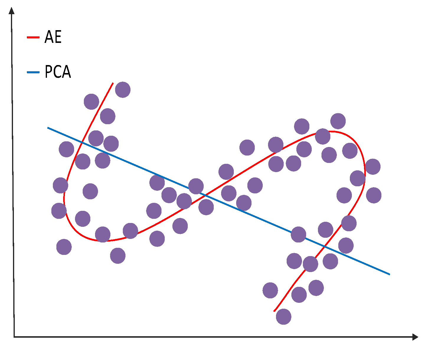
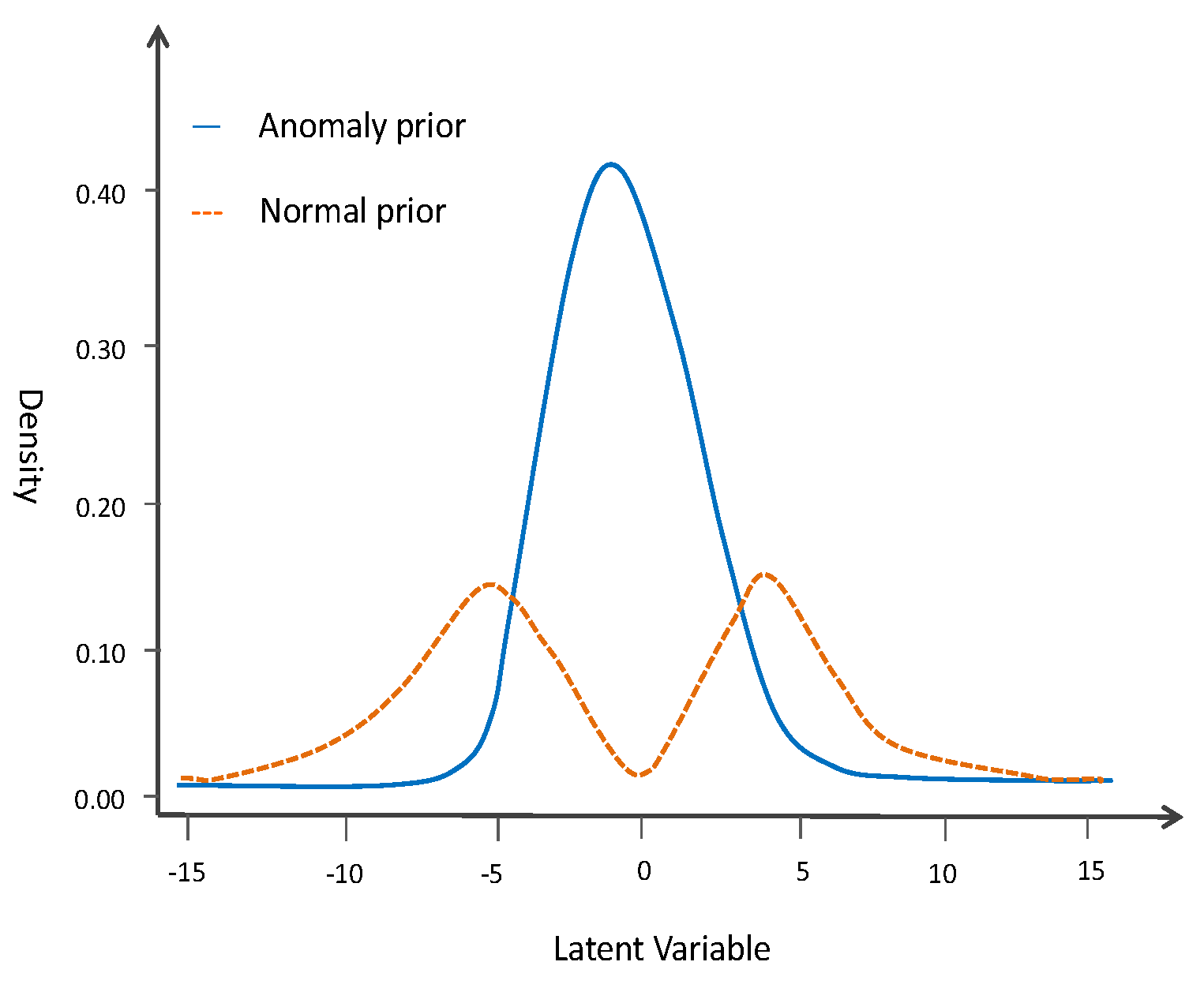
In neural networks, VAEs are feedforward acyclic neural networks. They are an unsupervised machine learning method. They can effectively extract very good data features and reduce the dimension of high-dimensional data. As opposed to AE, VAE’s latent space consists of a probability distribution of approximate data, while AE’s consists of a specific encoding of the input data. Figure 2 shows a sample of a prior distribution in Euclidean space of VAE latent vectors.

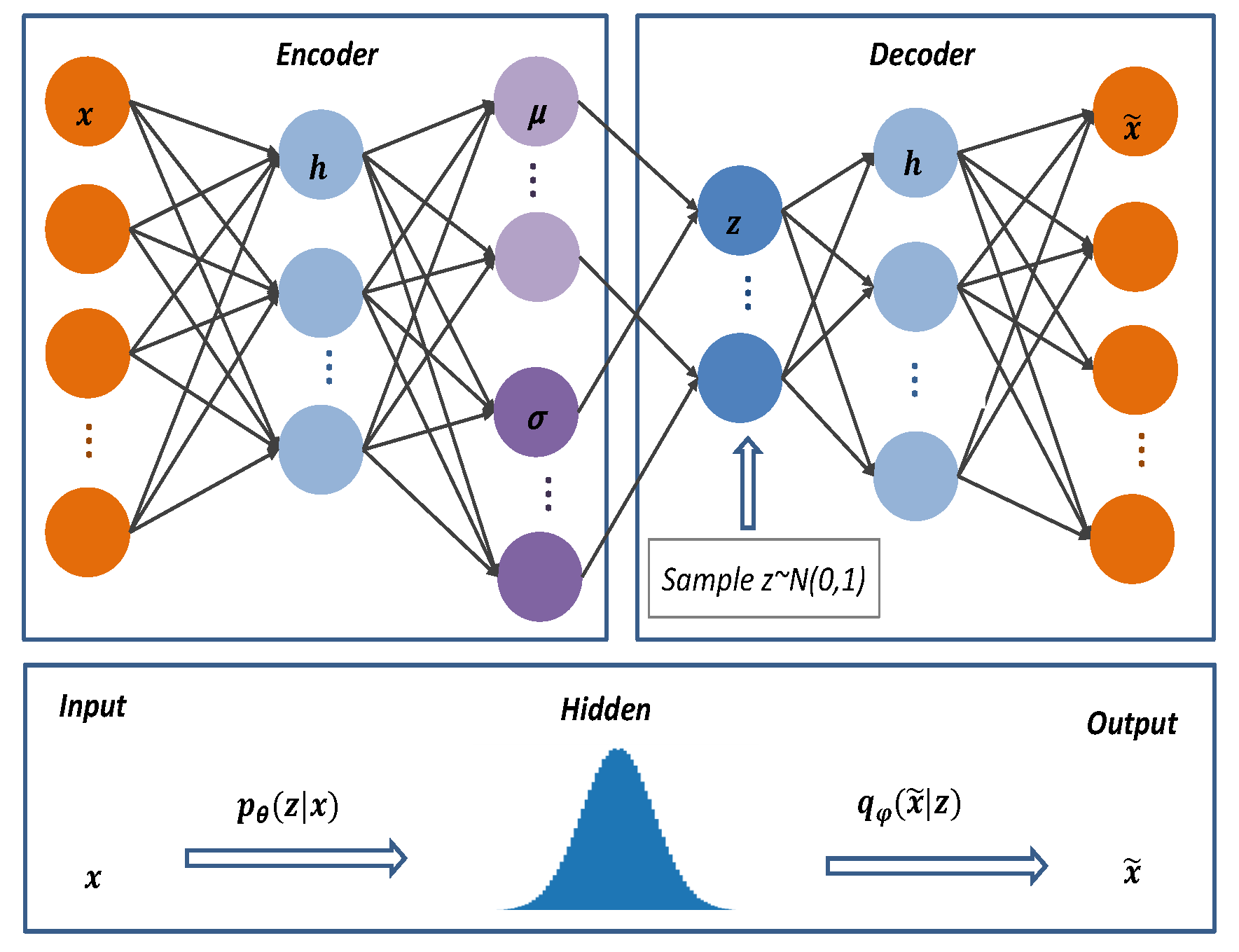
VAE’s structure resembles classic autoencoders with encoders, decoders, and latent spaces. The network structure of VAE is shown in Figure 3.

From Figure 3, $p_{\theta }\left(z|x\right)$ is the inferred network model known as the encoder. The original input data $X=\left\{x_1,x_2,...,x_n\right\}$ is mapped from the current space $R_n$ to the hidden space $R_h$ to obtain the variational probability distribution of the hidden layer z. As input x and hidden space Z are connected, the inferred model learns the joint probability distribution between them. $q_{\varphi }\left(x|z\right)$ is the generative network model, that is, the decoder. It performs sampling from the probability distribution $q_{\varphi }\left(z|x\right)$ of the hidden layer Z, and after sampling the hidden vector, z is decoded to produce an approximation of the target distribution $\tilde{X}$.

We applied the Bayesian formula as in Equation (1) to compute the probability distribution $p_{\theta }\left(z|x\right)$ of the hidden variable Z given the data X.

$$p\left(z|x\right)=\frac{p\left(x|z\right)p\left(z\right)}{p\left(x\right)}$$

(1)

We applied variational inference to approximate an unresolvable conditional probability distribution $q_{\varphi }\left(z|x\right)$ with a solvable distribution $p_{\theta }\left(z|x\right)$ since the input data distribution $p\left(x\right)$ is not computed as the dimensionality increases. We fitted the probability distributions $p_{\theta }\left(z|x\right)$ and $q_{\varphi }\left(z|x\right)$, applying KL divergence to determine the disparity between them and to minimize the difference as best as possible. As shown in Equation (2),

$$KL\left(q_{\varphi }\left(z|x\right)\left|\right|p_{\theta }\left(z|x\right)\right)=logp\left(x\right)+E\left[log{q}_{\varphi }\left(z|x\right)\right]-E\left[log{p}_{\theta }\left(z|x\right)\right]$$

$$=logp\left(x\right)+E\left[log{q}_{\varphi }\left(z|x\right)\right]-E\left[log{p}_{\theta }\left(z,x\right)\right]$$

(2)

The model parameters are trained by minimizing the difference between the two probability distributions. A smaller difference shows better parameters are obtained from training the VAE. Since X is certain, the first term in the equation $logp\left(x\right)$ is a fixed value, so the training objective becomes to minimize the last two items $E\left[log{q}_{\varphi }\left(z|x\right)\right]-E\left[log{p}_{\theta }\left(z,x\right)\right]$ of the equation, which is denoted as L. Then −L represents the lower bound of evidence $p\left(x\right)$. Here, minimizing L gives the maximized lower bound of evidence (ELBO), as shown in Equation (3):

$$Max\left[-L(\theta ,\varphi )\right]=E_{z\sim q_{\varphi }\left(z|x\right)}\left[log{p}_{\theta }\left(x|z\right)\right]-KL\left(q_{\varphi }\left(z|x\right)\left|\right|p\left(z\right)\right)$$

(3)

The first term of the equation is: $E_{z\sim q_{\varphi }\left(z|x\right)}\left[log{p}_{\theta }\left(x|z\right)\right]$, which indicates the continuous random samples of the probability distribution of the hidden space z. The second term reveals that the latent vector z is continuously sampled to ascertain that the probability of reconstructing the sample x is maximized, so that the post-validation distribution $p_{\theta }\left(z|x\right)$ and the prior distribution of $q_{\varphi }\left(z|x\right)$ are as close as possible. In order to construct the loss function of the model from this, we first consider the similarity between the input and the output and then make use of reconstruction loss to measure the difference between them. Secondly, due to the peculiarity of its coding layer, the variational autoencoder uses the latent loss to measure the “fitness” between the true probability distribution and the standard normal distribution. Consequently, the loss function of VAE ultimately consists of two items, as shown in Equation (4):

$$Loss=ReconstructionLoss+LatentLoss$$

$$Loss(\theta ,\varphi )=-E_{z\sim q_{\varphi }\left(z|x\right)}\left[log{p}_{\theta }\left(x|z\right)\right]+KL\left(q_{\varphi }\left(z|x\right)\left|\right|p\left(z\right)\right)$$

(4)

3.2. Genetic Algorithm

Genetic algorithm is considered a sort of heuristic randomized search technique that has natural selection and strong global optimization capabilities. Generally, it is carried out over multiple generations, where individuals evolve in a population until it is eventually capable of obtaining the optimal solution based on the fitness function. Figure 4 demonstrates the architectural diagram of the genetic algorithm, which comprises the following operations:

i.

Chromosome coding. The chromosome describes the subspace feature string of the outliers to be tested. We use the standard binary individual coding rules to code the subspace of the solved outliers. Each bit in the individual will take the binary numbers {0,1}, indicating whether its corresponding feature component is selected.

ii.

Fitness function. The genetic algorithm will perform N iterations during its operation, and each iteration will generate several chromosomes. Each chromosome generated in this iteration will receive a fitness score based on the fitness function. Then, only the chromosomes with high fitness are saved, and those with lower fitness are deleted. After the iterations, the chromosome quality will improve over time as the iterations continue.

iii.

Genetic operator. The use of genetic operators gives genetic algorithms the ability to evolve, including selection, crossover, and mutation operations. Individuals of the new generation are mostly produced by selection and mutation, while mutation is used to alter some gene positions in order to maintain diversity in the population and prevent premature convergence.

iv.

Evolution Termination. If the population converges, that is, no offspring with huge differences from the previous generations are generated, or the number of iterations reaches the upper limit specified, the evolution of the genetic algorithm will be terminated, and a set of solutions to the current problem will be obtained.

3.3. The Proposed VAEGA Model

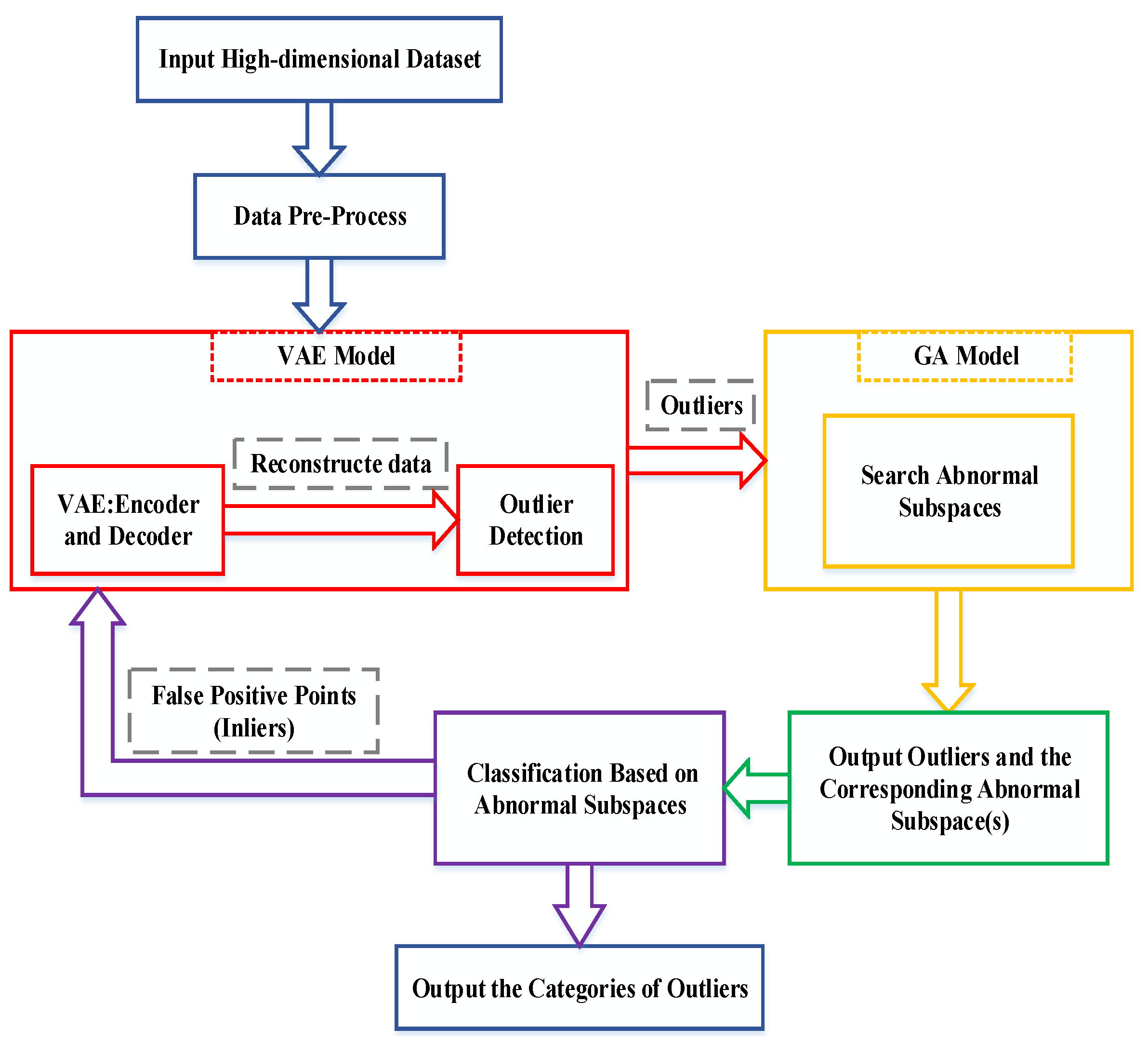
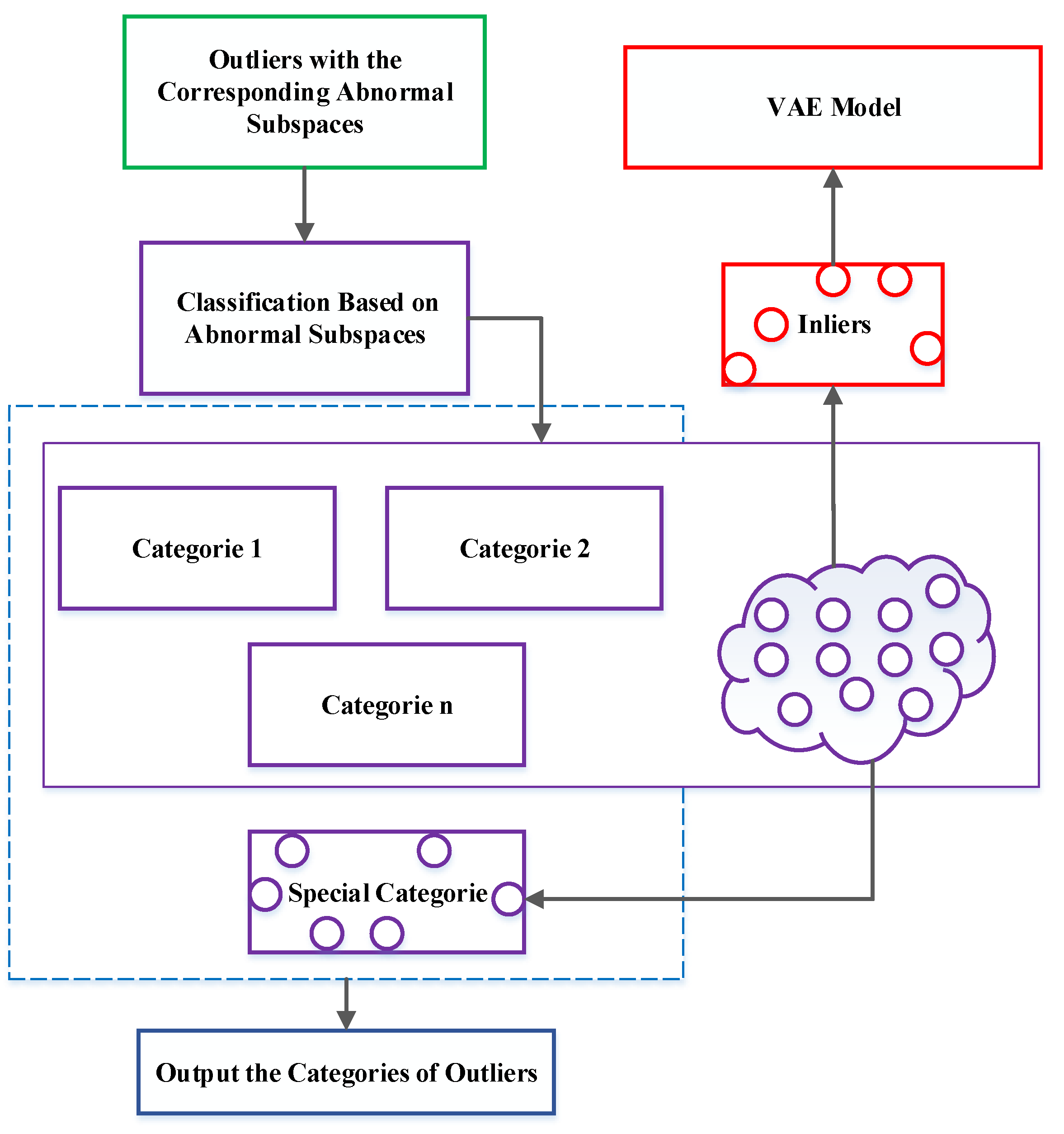
This section presents our proposed VAEGA model in detail. The model is applied to reduce the dimensionality challenges encountered by outlier detection in high-dimensional data. While focusing on improving the effectiveness of the outlier detection model from the perspective of data subspace, the heuristic optimization algorithm is used to obtain the abnormal subspace of outliers to solve the problem that high-dimensional outlier detection models generally lack interpretability.

The VAEGA model is defined as a model that combines a variational autoencoder and a genetic algorithm for the purpose of detecting outliers in high-dimensional data and searching for abnormal subspaces. Figure 5 shows the framework of the model.

The VAEGA model is divided into two modules. The first part is the VAE model, which executes the process of quickly filtering out the outliers. In the training phase, the VAE module uses a neural network to build a variational encoder $p_{\theta }\left(z|x\right)$ and decoder $q_{\varphi }\left(x|z\right)$. The unlabeled data are used as input for iterative optimization to learn the best encoding and decoding scheme and obtain the mean $\mu$, and standard deviation $\sigma$, of the input data x. This step effectively represents the distribution of high-dimensional input data and ameliorates the representation of the high-dimensional data. For real-valued sample data, assuming that the distribution function is a multi-dimensional Gaussian distribution, its indicators are shown in Equations (5)–(7) as follows:

$$p\left(z\right)=N(0,I)$$

(5)

$$q_{\varphi }\left(z|x\right)=N({\mu }_e,{\sigma }_e^2)$$

(6)

$$p_{\theta }\left(x|z\right)=N({\mu }_d,{\sigma }_d^2)$$

(7)

To optimize the weight parameters, we fit the data’s true probability distribution with a standard normal distribution. Through the use of stochastic gradient descent and backpropagation, the loss function of the model converged to a stable minimum value. The loss function of the VAE neural network is shown in Equation (8), and Equation (9) shows the KL divergence used to measure the two probability distributions.

$$L(\theta ,\varphi )=-{∥x-{\mu }_d∥}^2+KL\left(N\left({\mu }_e,{\sigma }_e\right)\left|\right|N(0,I)\right)$$

(8)

$$KL\left(N\left(X\right)\left|\right|ϵ\right)=\frac{1}{2}\left(tr\left[{\sigma }_e^2+{\mu }_e^T{\mu }_e-R_d-log\left|{\sigma }_e^2\right|\right]\right)$$

(9)

where a random variable X is normally distributed with a mean ${\mu }_e$ and standard deviation ${\sigma }_e$, $ϵ=N(0,I)$, $t_r$ is the trace of the matrix, and $R_d$ is the input data dimension. In Equation (8), the first item depicts the space between the reconstructed data and the input data. As a “reconstruction item” it tends to produce high performance in the encoding and decoding schemes. Regarding the second item, the KL divergence can be viewed as a penalty that regulates the hidden space.

It is important that we sample the latent vector z from $q_{\varphi }\left(z|x\right)$, which obeys the Gaussian distribution $z\sim q_{\varphi }\left(z|x\right)=N(\mu ,{\sigma }^2)$. The mean $\mu$ and variance $\sigma$ of z can be computed by the model, and the neural network relies on this sampling process to reverse optimize the variational autoencoder model. In this case, backpropagation for the model is impossible because sampling is not derivable. We then take into account that the results of sampling are derivable, which can be overcome by employing the reparameterization trick. The random variable z is sampled from the standard normal distribution N(0, 1) instead of the original distribution, and then the random variable $q_{\varphi }\left(z|x\right)$ undergoes the following transformation, as shown in Equation (10).

$$z=h_{\varphi }\left(\epsilon ,x\right)$$

(10)

From $\epsilon$ to z involves linear operations, which are derivable. The distribution of $\epsilon$ is deterministic and does not need to be learned. The sampled value of $\epsilon$ participates in the gradient descent, while the operation of sampling $\epsilon$ does not.

Using the trained VAE network model, we input the test data. The feature information of the normal data can be represented by latent vectors in latent space and reconstructed with minimal loss. However, outliers are difficult to represent in the latent space, resulting in huge errors between the reconstructed data and the original input data. Therefore, we can combine the reconstruction probability error and latent space information as a measure of the outlier degree of the data, denoted as $R{P}_i$, as shown in Equation (11).

$$R{P}_i=\frac{1}{M}\sum _{m=1}^{M}N\left(x_i\right|{\mu }_d\left[i,m\right],{\sigma }_d\left[i,m\right])$$

(11)

For comparability, we normalize the anomaly score $R{P}_i$ of each point to the range [0, 1] and re-denote it as $RP\_scor{e}_i$, as shown in Equation (12). As the anomaly score approaches 1, the abnormality of the data increases, making it more likely that it is an outlier. On the contrary, it indicates that the characteristics of the data are more normal.

$$RP\_scor{e}_i=\frac{R{P}_i-minR{P}_i}{MaxR{P}_i-minR{P}_i}$$

(12)

It is then compared to a threshold $\epsilon$, where $\epsilon$ is a metric used to control the model’s sensitivity to outliers. If the abnormal score $RP\_scor{e}_i$ of the candidate data is less than the threshold $\epsilon$, it means that the candidate data has a high degree of similarity with the normal sample and is marked as a normal value. If the abnormal score $RP\_scor{e}_i$ of the candidate data is greater than or equal to the threshold $\epsilon$, it means that the difference between the current data to be tested and the normal sample is large. This is then recorded as an outlier.

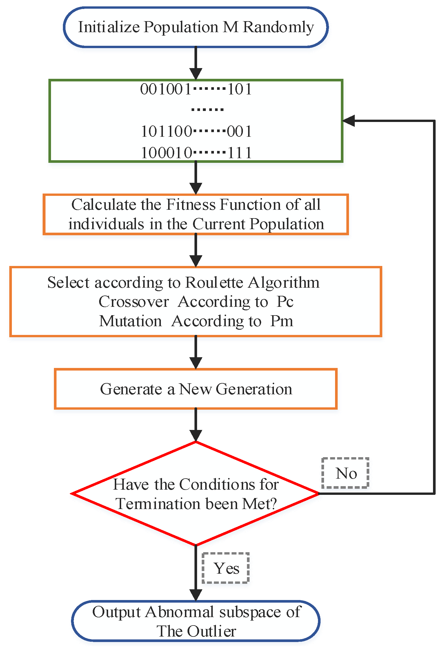
The second part of the model is the GA module, which takes as input the high-dimensional abnormal data obtained by the previous module and trains the genetic algorithm to search the abnormal subspace of high-dimensional outliers. The abnormal subspace of the outliers can provide the basis for the analysis of abnormal causes. Figure 4 shows the flow of its search algorithm.

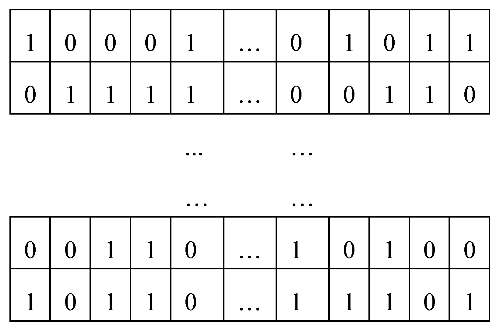
By analyzing the subspace of the outliers, we found that there are only two states of the subspace feature components, so the binary encoding rules were chosen to establish the mapping relationship between data subspaces and encoding strings. The problem of solving the abnormal subspace of data is transformed into the problem of searching for the optimal individual through genetic algorithm. Firstly, $N_{Gen}$ individuals containing $N_{dim}$ genes are randomly generated to form an initial population representing feasible solutions of the abnormal subspace, where $N_{Gen}$ is the population size and $N_{dim}$ is the dimension of the full data space. Each chromosome consists of {0,1}, where 1 means that the feature component was selected. The initial population generation is shown in Figure 6.

To determine the fitness function for the target problem, the second part analyzes the target problem. We redefine the metric to be the fitness function of the genetic algorithm since our goal is to obtain the anomalies of the current candidate subspace to determine whether it has been eliminated.

Definition 1.

Subspace Outlying Degree, SOD. In this work, $D^k$ (the distance between the point to be measured and the k-th nearest neighbor) is used as an outlier metric, which is called the subspace outlying degree. Since there is likely to be a high numerical outlier distance within a subspace, it is difficult to compare outliers between different subspaces. Therefore, to improve the comparability of the abnormal subspace SOD, the subspace abnormality SOD is defined as the ratio of $D_s^k\left(p\right)$ at a given point p to the average(avg) $D_s^k\left(Data\right)$ in the data set denoted as Data in the same subspace s, as shown below:

$$SOD\left(s.p\right)=\frac{D_s^k\left(p\right)}{avg\left(D_s^k\left(Data\right)\right)}.$$

(13)

The higher the ratio, the higher the $D^k$ for the point sample p compared to other points, so the higher the outlier value of p, and vice versa. Our definition of SOD derives from the definition of the outlier subspace. Given the input data set denoted as Data, the parameter denoted as n is the dimension of the data set, and k is the number of adjacent data points. If there is no subspace s’, such that SOD(s’, p) > SOD(s, p), then the abnormal subspace of a given data point p is s.

The fitness function SOD is calculated for all individuals in the current population and sorted by size. Determine whether the chromosome corresponding to $SO{D}_{top}$ in the current generation population satisfies the stopping condition. If so, decode the chromosome to obtain the abnormal subspace of candidate outliers. Otherwise, the VAEGA model will utilize genetic operators to generate a new generation of subspace populations. The specific steps are as follows. We calculate the fitness function SOD of each chromosome and then use the current ratio of each individual’s $SO{D}_i$ value to the sum $SO{D}_{sum}$ as the individual’s selection probability $P_{v_i}$, as shown in Equation (14).

$$P_{v_i}=\frac{SO{D}_i}{SO{D}_{sum}}$$

(14)

The larger the value, the higher the abnormal degree of the candidate outlier in the current subspace, and the higher the probability of the individual being selected to be inherited by the next generation.

The selection of individuals is a random process, which means individuals with high SOD values may be lost in the selection process. Hence, we add a mechanism for optimal retention selection, which directs the top N outstanding individuals with SOD values in the previous generation into the new generation population.

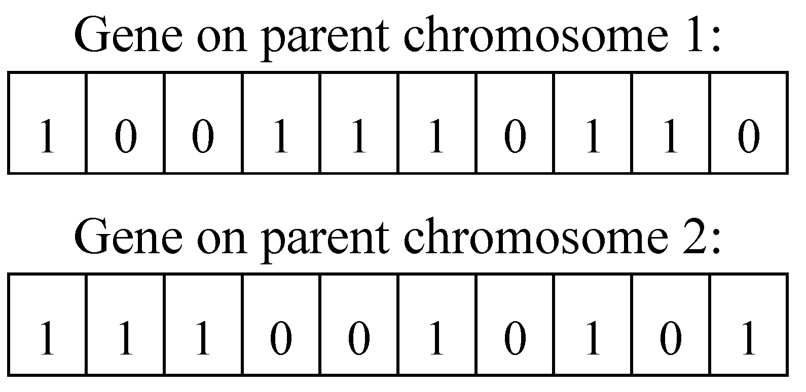
Then we use the non-replacement remainder rule to select population N chromosomes to inherit into the next generation population. In the new generation population, our work randomly selects an even number of parent chromosomes without repetition and performs a uniform crossover operation according to the crossover probability $P_c$. The resulting child chromosomes will be put into a new generation of populations. The binary uniform crossover operation is shown in Figure 7.

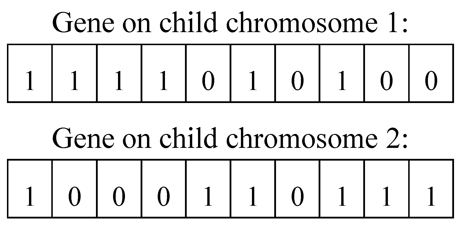
It is assumed that the random probability of genes at positions 2, 3, 5, 8, and 9 is greater than the crossover probability $P_c$. Then, the genes at positions 2, 3, 5, 8, and 9 are exchanged to form two new child chromosomes in Figure 8.

To generate distinct evolutionary directions for populations, some children chromosomes are picked at random for single point mutations based on mutation probability $P_m$. The new generated population continues to repeat the above process until the algorithm converges or the stopping condition is satisfied.

By doing so, an optimal abnormal subspace solution that meets the search objective is obtained.

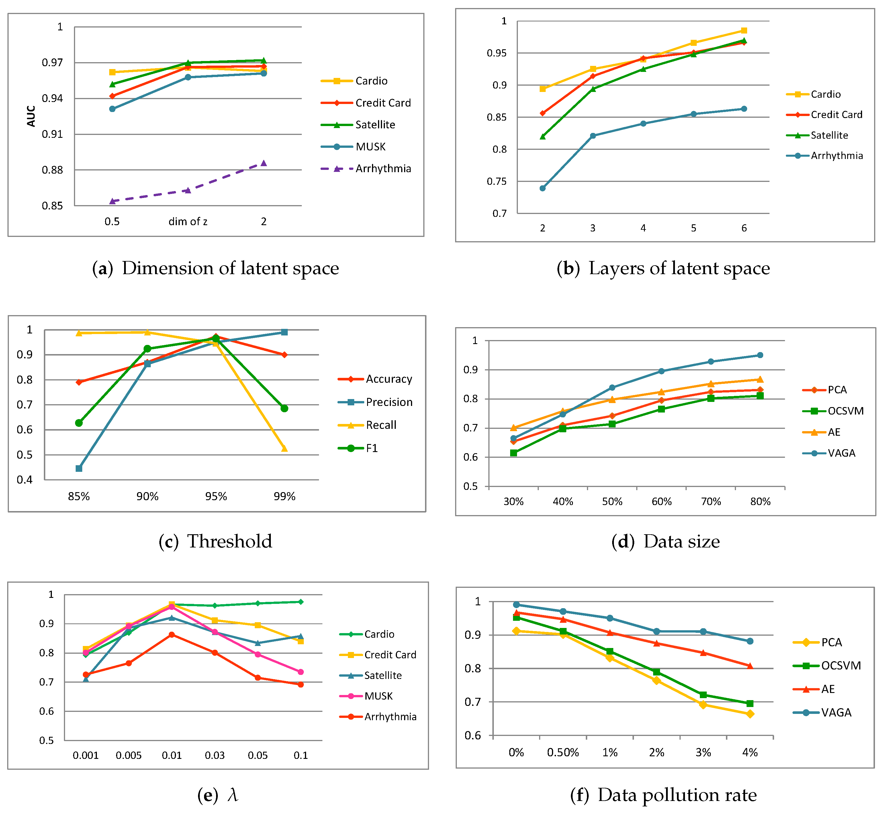
The most challenging step in using the genetic algorithm to search for anomalous subspaces is to calculate the fitness of each individual subspace. When we calculate the fitness SOD of candidate values in the current subspace, we need to scan the entire dataset, but the scale of high-dimensional datasets is usually large. For severely imbalanced datasets, we use a random multiple sampling technique, replacing the entire dataset with a randomly sampled dataset. By using random multiple sampling, the subjective bias of the samples obtained by single sampling can be reduced to a certain extent, so that the sample subset can represent the entire data set. By applying the random sampling method, it is possible to more efficiently calculate the abnormality degree of the current abnormal point subspace to measure and evaluate fitness more quickly. Nevertheless, we expect that the quality of the search results may be slightly affected, as will be verified in the experimental section.

3.4. False Positives Feedback Mechanism

In order to refine the interpretability of the VAEGA model results, we subclassify the outliers according to the set of anomaly subspaces searched by the GA layer (see Algorithm 1). The structure diagram of this mechanism is shown in Figure 9.

Algorithm 1 Search Subspace Process

Require:  Outlier dataset O = $\{o_1,o_2,...,o_n\}$; Ensure:  Abnormal subspace set $AS$ = $\{{\left(as\right)}_1,{\left(as\right)}_2,...,{\left(as\right)}_n\}$; 1: Initialize the population $Gen$, the number of individuals is $N_{Gen}$, and set the crossover probability $P_c$ and mutation probability $P_m$; 2: for$i=1$ to n do 3: Epoch = 1 4: while$Epoch<Ma{x}_{Epoch}$do 5:   Calculate the fitness function for each chromosome 6:   if $SO{D}_{top}$ satisfies the optimal solution then 7:     $a{s}_i$ = individual $v\_\left(SO{D}_{top}\right)$ decoded into abnormal subspace representation 8:   else 9:     Calculate the probability of selection of a chromosome 10:     Use the best retention to select the value of $p_{v_i}$ the top $N_{Best}$ chromosomes into the next generation 11:   Select $N_k$ chromosomes using no-replacement remainder selection rule among the remaining chromosomes 12:   for $j=1$ to ($N_{Gen}-N_{Best}-N_k$) do 13:   Randomly select two parent chromosomes 14:   Perform gene crossover according to $P_c$ and uniform crossover rules to form two new chromosomes and join the cenozoic population 15:   end for 16: Perform mutation operation on random m chromosomes in the population according to $P_m$ 17: Epoch = Epoch + 1 18: end while 19: end for 20: return Abnormal subspace set $AS$ and weight values

The first step is to match candidate outliers’ abnormal subspace features with those of existing outlier classes. A point will be assigned to the outlier class if it has the same abnormal features in its subspace. Otherwise, a new outlier subclass will be generated. This step will continue until all outliers are classified. We merge subclasses that contain only one outlier into a special class.

In the second step, we focus on examining the special classes based on the subclassification results above. The points in the abnormal subspace in which each feature component is within its normal range are screened out, that is, those points whose abnormal feature values are within $\pm 3\sigma$ of the corresponding feature data distribution. The selected points are deemed as misjudgments of the model and form a set of false positive points. After that, we use the set of false positive points to optimize the parameters of the VAE outlier detection module in order to reduce the false positive rate of the VAEGA model.

In the final step, special filtered classes and other subclasses will be used to analyze the causes of anomalies. Often, outliers that occur in a special class can be more informative since they often result from the properties of the data themselves. People may be able to avoid substantial losses by paying attention to special outliers and taking action to remedy them as soon as possible.

4. Experimental Design

In this section, we will assess the performance of the VAEGA model proposed in this paper based on experiments. The section will include an introduction to the real data set and comparative benchmark models used in the experiment, as well as verification of the accuracy of the VAEGA model in unsupervised outlier detection and the ability to search for abnormal subspace.

4.1. Datasets

To evaluate the performance of the method proposed in this work, we used five real high-dimensional datasets: (1) Cardio; (2) Creditcard; (3) Satellite; (4) MUSK; (5) Arrhythmia.

The Creditcard fraud dataset comes from Kaggle, and the other four datasets come from the ODDS library (http://odds.cs.stonybrook.edu/ accessed date: 20 October 2021). The detailed information about the datasets is presented as follows. Some key statistics of the datasets are also given in

Table 1. Dataset information.

Dataset	N	Dim	Outliers (%)
Cardio	1831	21	176 (9.6%)
Creditcard	284,807	32	492 (0.17%)
Satellite	5100	36	77 (1.5%)
Arrhythmia	452	279	66 (15%)
MUSK	3062	166	97 (3.2%)

.

Cardio: The Cardio dataset is a 21-dimensional measurement dataset containing fetal heart rate signature (FHR) and maternal uterine contraction signature (UC) in the medical field ECG, which has been labeled by obstetric experts. Among them, the pathological class is used as the abnormal class of the dataset, with 176 data points. Except for the suspicious data class, which is removed, other data classes in the dataset are used as normal samples for training.

Creditcard: Kaggle provided two-day credit card transaction information for European cardholders in September 2013. The data set contains 32 attributes, of which 492 out of 284,807 transactions were stolen. The data set is very unbalanced, with outliers accounting for 0.172% of all transaction data.

Satellite: The Satellite dataset is an Earth resource satellite dataset containing 36 attributes. Since the data proportions of the three categories 2, 3, and 4 are the smallest, they can be combined into anomalous categories, and other categories are used as normal samples for training.

Arrhythmia: The dataset is a multi-class classification dataset with a dimension of 279. The smallest categories, namely 3, 4, 5, 7, 8, 9, 14, 15, are merged to form an outlier category, and the remaining categories are merged to form a normal category.

MUSK: There are 166 dimensions in the Musk dataset, and there are both Musk datasets and non-Musk datasets. Inliers consist of the non-musk classes j146, j147, and j252, while outliers consist of the musk classes 213 and 211.

After we preprocessed the data, there were no missing values in all the datasets, and all the datasets were scaled to [0, 1].

4.2. Experimental Settings

In order to create the model, we used Tensorflow 1.14.0 and Python 3.7. We randomly selected 80% of the data to be the training set and 20% for the testing set. For the training phase, we set the hidden space Z of the VAE to two and the input dimension of the neuron unit of the hidden layer h to half. We apply the ReLU max(x, 0.1x) activation function and SGD optimizer to train the VAE. For the other parameters of the autoencoder, we use the default values. As described in Section 3.3, the anomaly score is determined in the testing phase, and the threshold is 95% of the root mean square error.

Our experiments compare VAEGA with 9 outlier detection benchmark models, including OC-SVM [18], PCA [22], ABOD [41], HBOS [42], GAN [43], MOGAAL [44], DSEBM [28], AE [25], and pure VAE. PCA and OC-SVM are traditional outlier detection methods, ABOD and HBOS are distance-based methods to reflect the limitations of the distance of high-dimensional data space, and GAN and MOGAAL are outlier detection models based on generative adversarial networks. DSEBM, AE, and pure VAE are reconstruction-based outlier detection methods. For traditional methods such as PCA and OC-SVM, we use Scikit-Learn in TensorFlow to implement. For other methods besides the proposed VAEGA model, we use Tensorflow and python to implement them. The optimizer, learning rate, batch size and number of iterations used by the other methods are the same as those of the VAEGA model, except that the parameters of MOGAAL refer to the recommended settings of [1]. For comparability, AE, pure VAE and DSEBM share the same network structure and the same hidden layer units as VAEGA. The details of the baseline model are as follows:

(1)

Traditional outlier detection methods: The OC-SVM method is a well-known kernel-based outlier detection method. Our experimental task uses the radial basis function (RBF) kernel, the abnormal rate $\nu$ is set to 0.05, and uses the technique proposed by [18] to adjust the Gaussian kernel parameter $\sigma$. PCA is a linear dimensionality reduction method that can be used to extract the main feature components of the data. The eigenvector matrix is compressed into h dimension, which is the same as the hidden space dimension of the VAE layer in the proposed method. PCA uses reconstruction error as an abnormal score.

(2)

Distance-based: The ABOD performance of the probabilistic method is significantly affected by the neighborhood size, and we set its parameter to 16 in comparative experiments. The HBOS method selects the number of commonly used neighbors as 10.

(3)

Generative adversarial network-based methods: In the comparative experiment, the GAN and VAEGA models basically have the same network structure, but the output layer of the discriminator in GAN is set to a one-dimensional structure. The configuration of MOGAAL can be found in [44]

(4)

Reconstruction-based methods: DSEBM is a deep-structured energy-based model, which is one of the recent deep-learning methods for unsupervised outlier detection. In DSEBM, the energy-based models (EBM) energy score of a sample is used as a criterion for detecting outliers. Autoencoder is an unsupervised nonlinear learning algorithm for data dimensionality reduction. The neural network parameters of the training encoder and decoder are the same. AE uses the error before and after reconstruction as an abnormality criterion. The training method, parameters, and the number of hidden layer units of pure VAE are the same as those of the VAEGA model.

In the experiment, we search for abnormal subspaces using the Creditcard dataset, which has perfect data preprocessing for further evaluation of the model. The input of the GA layer is the set of outliers obtained through the outlier detection of the VAE layer. The GA layer starts with a population of 100, and the distance encoding is determined by the input dimension dim of the outlier. The fitness function calculates the SOD for each subspace. To identify individuals with better performance in the existing generation and position them in the next generation, the selection operator uses the remainder nonreplacement selection method and the optimal retention method. We set the crossover probability $P_c$ to 0.6 and the mutation probability $P_m$ to 0.01. Using the random module function, we can achieve multi-sample random samples.

5. Results and Discussions

5.1. Experimental Evaluation

In order to evaluate the model’s performance and the benchmark models, we consider the following five indicators in our experiment: accuracy, recall rate, F1 score and the AUC. Each indicator’s best results are highlighted in bold.

Table 2. Accuracy results of outlier detection for 10 models on 5 datasets.

Methods	Cardio	Credit Card	Satellite	MUSK	Arrhythmia
PCA	0.886	0.831	0.683	0.892	0.808
OC-SVM	0.927	0.811	0.710	0.90	0.809
ABOD	0.923	0.907	0.745	0.735	0.647
HBOS	0.854	0.862	0.746	0.716	0.698
GAN	0.697	0.659	0.427	0.796	0.656
MOGAAL	0.730	0.734	0.797	0.814	0.702
DSEBM	0.837	0.883	0.705	0.899	0.773
AE	0.798	0.867	0.764	0.931	0.816
VAE	0.803	0.901	0.766	0.969	0.895
VAEGA	0.851	0.950	0.792	0.961	0.879

,

Table 3. AUC of 10 models for outlier detection on 5 datasets.

Methods	Cardio	Credit Card	Satellite	MUSK	Arrhythmia
PCA	0.832	0.892	0.675	0.881	0.805
OC-SVM	0.975	0.878	0.893	0.866	0.808
ABOD	0.948	0.562	0.972	0.726	0.801
HBOS	0.899	0.913	0.895	0.869	0.847
GAN	0.618	0.752	0.776	0.767	0.776
MOGAAL	0.792	0.854	0.971	0.880	0.854
DSEBM	0.942	0.84	0.6375	0.847	0.762
AE	0.840	0.922	0.950	0.922	0.812
VAE	0.840	0.958	0.962	0.933	0.871
VAEGA	0.966	0.966	0.970	0.957	0.863

,

Table 4. F1 scores of 10 models for outlier detection on 5 datasets.

Methods	Cardio	Credit Card	Satellite	MUSK	Arrhythmia
PCA	0.861	0.831	0.723	0.819	0.753
OC-SVM	0.898	0.812	0.439	0.799	0.795
ABOD	0.647	0.689	0.657	0.703	0.718
HBOS	0.703	0.770	0.490	0.763	0.762
GAN	0.500	0.791	0.226	0.795	0.700
MOGAAL	0.578	0.677	0.627	0.731	0.688
DSEBM	0.909	0.782	0.732	0.782	0.742
AE	0.661	0.872	0.589	0.861	0.741
VAE	0.820	0.901	0.817	0.916	0.831
VAEGA	0.805	0.927	0.827	0.940	0.813

and

Table 5. Recall of 10 models for outlier detection on 5 datasets.

Methods	Cardio	Credit Card	Satellite	MUSK	Arrhythmia
PCA	0.890	0.830	0.768	0.829	0.751
OC-SVM	0.957	0.827	0.773	0.800	0.852
ABOD	0.983	0.895	0.893	0.797	0.805
HBOS	0.625	0.675	0.853	0.816	0.830
GAN	0.903	0.895	0.747	0.799	0.753
MOGAAL	0.455	0.543	0.493	0.674	0.682
DSEBM	0.869	0.781	0.758	0.782	0.747
AE	0.830	0.878	0.840	0.867	0.739
VAE	0.801	0.905	0.897	0.917	0.780
VAEGA	0.938	0.936	0.853	0.924	0.773

show the results of the experiment.

In order to determine the capability of searching abnormal subspace using the trained GA layer based on the outlier detection model, we compare it to the ground truth for the outliers detected by the outlier detection model. Obtaining the ground truth requires traversing all low-dimensional subspaces in the dataset and sorting the outlier degrees. Outlier degrees correspond to accurate abnormal subspaces and are given by the outlier degree in the top 1. In Table 5, a subspace in the ground truth of abnormal subspaces is shown. Table 5 shows the three-dimensional subspace component [V4, V5, V10]. A relatively high outlier degree in the data with serial number of 86 suggests an abnormality may exist in the V4, V5, and V10 feature subspace. In

Table 6. An example: abnormal subspace ‘V4,V5,V10’ in the ground truth of the abnormal subspaces for the dataset.

	Outlier Data	Outlier Degree	Data Serial Number
1	[4, 5, 10]	9.10	86
2	[1, 2, 7]	4.33	112
3	[0, 1, 15]	4.02	302
4	[1, 3, 22]	3.56	29
5	[0, 1, 5]	3.41	54

, a comparison of the accuracy is made between the ground truth and the abnormal subspaces of the outliers set searched by the genetic algorithm.

5.2. Experiment Analysis

From Table 2, Table 3, Table 4 and Table 5, the results from our experiments show that the VAEGA model surpasses the other benchmark models, particularly in terms of accuracy on all five datasets. Our VAEGA model utilizes a variational method that offers better flexibility for underlying generative models. It employs latent variables with a small amount of noise to generate data more reasonably in order to make the VAEGA model more effective. We found that on datasets with low outlier rates (such as the credit card fraud dataset), the model maintains good performance. By contrast, PCA’s performance in detecting linear outliers is generally lower than other benchmark models, indicating that it is difficult to determine the intrinsic relationship between data points. The “curse of dimensionality” limits the outlier detection capability of OC-SVM. It performs well on the Cardio, CreditCard, and Satellite datasets but produces inferior results on the high-dimensional Arrhythmia dataset. Distance-based ABOD and HBOS perform slightly better, but they also suffer from dimensionality problems. Another reason for unstable performance is that such methods usually pre-end the training data with prior knowledge. The performance of these algorithms may be adversely affected by high-dimensional data or by data that have a distribution that is inconsistent with their prior knowledge. In contrast, the remaining five neural network-based methods do not demand strict distribution assumptions; therefore, they can perform better with high-dimensional datasets or datasets whose distributions are very different.

OC-SVM, on the other hand, has limited performance because of the curse of dimensionality. The AE model with low-dimensional information and dimensionality reduction reconstruction error and the energy-based DSEBM-e model perform well on multiple data sets. From the results, the methods based on dimensionality reduction perform much better. In VAEGA, the VAE layer utilizes the variational approach, which offers higher flexibility in the potential generation model, thereby improving outlier detection. Compared to the unimproved pure VAE, the VAEGA model achieves an average performance improvement of around 3%. We observe that on datasets with low outlier rates (such as credit card fraud) the model performs well. Furthermore, unlike other benchmark models, our proposed method can identify outlier features and evaluate the causes of data anomalies.

Based on the analysis of the experimental results from multiple datasets, the adversarial network-based methods—GAN and MOGAAL—showed to be less effective in detecting outliers compared to reconstruction-based methods, such as DSEBM, AE, VAE and VAEGA. The analysis showed that GANs lack reasoning about the training data in the hidden space, so they learn an incomplete data distribution, which leads to mode collapse. In addition, the GAN mislabels normal data as abnormal data, resulting in false positives in outlier detection results. The MOGAAL method, on the other hand, tries to elude the mode collapse by stopping the optimization of the generator before convergence to better learn the distribution of normal data and extends the network structure to multiple generators with different objectives from the initial single generator. Consequently, MOGAAL’s detection results outperform the ordinary GANs; however, the caveat is that it is difficult to know for certain what the model has learned, which leads to uncertain experimental results. Thus, there is still a performance gap compared with the reconstruction-based neural network models AE, VAE, and DSEBM. This is because reconstruction-based methods combine latent space information and reconstruction error to detect outliers.

Unsupervised outlier detection will, however, generate some misjudgment points if the threshold is set too high. Our improved VAEGA model establishes a genetic algorithm to search the abnormal subspace for the outlier set containing the misjudged points and classify the outliers in accordance with the abnormal subspace. Misjudged points are considered outliers that cannot form clusters in the classification results. In order to improve the model’s performance, the VAEGA model feeds the detected misjudgment points to the VAE layer for parameter adjustment. The reason for the slight improvement is that we cannot eliminate all misjudgment points through a unified standard when classifying outliers based on abnormal subspaces. Filtering out too few false positives or removing some of the features of false positives will have little effect on the weight adjustment of upper-layer feedback, which will result in an insufficient improvement in model performance. As a result, when training the model, we should use a large amount of data to ensure that important outliers are not isolated cases before formulating more effective criteria to filter false positives. Our proposed VAEGA model can output abnormal subspace features for analyzing data anomalies, whereas other benchmark models lack the ability to locate outliers.

In GA, the search for abnormal subspaces uses a heuristic search instead of traversing all the possible subspaces, which can save time and memory. As shown in

Table 7. An analysis of the calculated SOD results before and after random sampling was used.

Scope of Data	Accuracy
Complete sample dataset	0.859
Random sample sub dataset	0.823

, 85.95% accuracy can be achieved when comparing the abnormal subspaces obtained using the genetic algorithm with the standard set. The results demonstrate that our proposed method can obtain abnormal subspace features much more quickly since the search cost is greatly reduced. In addition, the fitness function of the GA for calculating the subspace fitness in the VAEGA experiment makes use of the redefined SOD measurement. A subspace with the highest SOD value is returned as the abnormal subspace for each detected outlier. This increases the comparability of the outlier measure in comparison to simply calculating the outlier degree. Furthermore, with the progress of evolution, we can see in the three datasets an increase in the number of individuals with high fitness, which indicates that our approach features good convergence. By taking advantage of this good convergence, we are able to find the abnormal subspaces of the detected outliers without having to explore a large number of subspaces.

Additionally, we use a random sampling method in our work to speed up the calculation of fitness functions of subspaces in the genetic algorithm. As illustrated in Table 7, the accuracy of searching the abnormal subspace only decreased by 0.036. Hence, it shows that the random sampling of the dataset has little impact on the final search results, but it saves running time and minimizes the calculation cost. For this reason, it is feasible to use randomly sampled samples as an alternative to the entire subspace data.

5.3. Sensitivity Analysis

The hidden layer of the VAEGA model is critical for training the model. It relies on the outlier detection module to compress the original high-dimensional data into the latent space. We retrain the VAEGA model by adjusting the dimension dim of the hidden layer z to half and twice. It can be seen from Figure 10a that reducing the dimensionality of the hidden layers to half of the experimental setting results in a decrease in outlier detection accuracy. The performance of outlier detection results on other datasets does not substantially improve with doubling the hidden layer dimension z, except for the Arrhythmia dataset of dimension 275. This is due to the data being prone to overfitting as a result of the high dimensionality of the hidden layer. The model’s performance will decrease if it is too low since the hidden layer will not learn enough from the input data. In addition, we progressively adjust the number of hidden layers from two to six in the VAEGA model. Figure 10b illustrates how the outlier detection performance is poor when there are just two hidden layers in the VAEGA model but improves as more layers are added. This is because the network layers do not suffice to fully learn the information contained in the training data. Generally, the number of layers and the size of the latent space do not have a significant effect on the results as long as the neural network is large enough. Thus, a reasonable setting of the neural network size of the model can lead to a robust network structure.

In the VAEGA model, VAEGA’s $ϵ$ threshold is determined by the proportion of outliers in the dataset. Observing Figure 10c, it is seen that the higher the threshold $ϵ$ is set, the higher the detection accuracy of the model, and the relative recall rate will be greatly reduced. Based on Figure 10c, it can be observed that the higher the threshold is set, the higher the model’s detection accuracy, and the lower the relative recall rate. Nevertheless, after exceeding the 99% threshold, the accuracy will fluctuate. When the threshold is set to 99%, the limit of outlier detection is higher, and only outliers with obvious anomalous characteristics (high anomaly scores) will be detected. Although this will lead to fewer errors in the model, it will leave most outliers unidentified. Increasing the threshold setting in the model to 85% will result in a higher rate of false positives. Therefore, setting the thresholds to 90% and 95% anomaly percentages is reasonable for the VAEGA model. However, because of the low outlier rate in the selected data set, the threshold is set at 95% in order to maintain the indicators in a more balanced position and minimize the impact of human factors on the model’s performance.

Additionally, we verify the influence of the training data size on the VAEGA model performance on the Creditcard dataset, which consists of 200,000 records. As can be seen in Figure 10d, the higher the number of training samples, the higher the learning ability and accuracy of the outlier detection model. In this sense, a sufficient amount of training data are needed to ensure that the learning task performs robustly and achieves better results. A crucial hyperparameter in the VAEGA model is $lambda$, which is obtained from training the VAE, and the value of $gamma$ is fixed at 0.01. From Figure 10e, it can be seen that the anomaly detection model performs best when lambda = 0.01, and its accuracy decreases below this value.

To test the model’s sensitivity when the data are polluted, we retrain the model using training data containing varying levels of noise. In Figure 10f, the drop in the curve shows that contaminated training data negatively impacts detection accuracy, with larger impacts on the model as contamination rates increase. It should be noted, however, that the OCSVM is more robust to tainted input data than any of the other three methods, while reconstruction-based models are also susceptible to tainted input. This is because the OCSVM model ignores a certain amount of noise when learning the boundaries of training data, whereas the AE and VAEGA models work alongside noise to reduce the reconstruction error across the whole set of training data. In practice, because data labels are costly to acquire, it is difficult to obtain completely clean data for outlier detection. In addition, high-dimensional data is usually unbalanced. Since there is a large amount of normal data compared to the abnormal data within the data set, the pollution rate is lower and the learning ability of the model is less impacted.

6. Conclusions

This paper proposed a method for detecting outliers in high-dimensional space and for searching abnormal subspaces in high-dimensional space. For high-dimensional data with dimensionality challenges, a variational autoencoder was used as an effective dimensionality reduction technique. Then, a genetic algorithm (GA) was used to detect outliers by searching subspaces for the detected outliers by the variation autoencoder. To accelerate the computation significantly, the SOD function was redefined as the fitness function to assess the degree of abnormality of subspaces in the genetic algorithm, and random sampling was used to improve the performance. After classifying the detected outlier by using the searched abnormal subspaces, false positives are able to be detected. The autoencoder then uses these data to further improve its detection capabilities. The results of experiments carried out on several benchmark datasets with high dimensions revealed that our proposed model can effectively detect outliers in high-dimensional data. When compared to other state-of-the-art methods, our model achieved an accurate abnormal subspace for outliers. In our future research work, we will concentrate on the abnormal subspaces of outliers and classify the outliers using clustering methods to classify the abnormal subspaces. In addition, we plan to vary the number of outliers and try different types of distribution models to observe the effect on the model. We also plan to explore the causes of the abnormalities and increase their interpretability.

References

1. Hawkins, S.; He, H.; Williams, G.; Baxter, R. Outlier detection using replicator neural networks. In Proceedings of the International Conference on Data Warehousing and Knowledge Discovery, Aix-en-Provence, France, 4–6 September 2002; pp. 170–180. [Google Scholar]
2. Bah, M.J.; Wang, H.; Zhao, L.H.; Zhang, J.; Xiao, J. EMM-CLODS: An Effective Microcluster and Minimal Pruning CLustering-Based Technique for Detecting Outliers in Data Streams. Complexity 2021, 2021, 9178461. [Google Scholar] [CrossRef]
3. Dai, J.; Song, H.; Sheng, G.; Jiang, X. Cleaning method for status monitoring data of power equipment based on stacked denoising autoencoders. IEEE Access 2017, 5, 22863–22870. [Google Scholar] [CrossRef]
4. Mahmoodi, K.; Ghassemi, H. Outlier detection in ocean wave measurements by using unsupervised data mining methods. Pol. Marit. Res. 2018, 25, 44–50. [Google Scholar] [CrossRef] [Green Version]
5. Almusallam, N.Y.; Tari, Z.; Bertok, P.; Zomaya, A.Y. Dimensionality reduction for intrusion detection systems in multi-data streams—A review and proposal of unsupervised feature selection scheme. Emergent Comput. 2017, 24, 467–487. [Google Scholar]
6. Sun, J.; Wang, X.; Xiong, N.; Shao, J. Learning sparse representation with variational auto-encoder for anomaly detection. IEEE Access 2018, 6, 33353–33361. [Google Scholar] [CrossRef]
7. Liu, S.; Hooi, B.; Faloutsos, C. Holoscope: Topology-and-spike aware fraud detection. In Proceedings of the 2017 ACM on Conference on Information and Knowledge Management, Singapore, 6–10 November 2017; pp. 1539–1548. [Google Scholar]
8. Osada, G.; Omote, K.; Nishide, T. Network intrusion detection based on semi-supervised variational auto-encoder. In European Symposium on Research in Computer Security; Springer: Cham, Switzerland, 2017; pp. 344–361. [Google Scholar]
9. Schlegl, T.; Seeböck, P.; Waldstein, S.M.; Schmidt-Erfurth, U.; Langs, G. Unsupervised anomaly detection with generative adversarial networks to guide marker discovery. In Proceedings of the International Conference on Information Processing in Medical Imaging, Boone, NC, USA, 25–30 June 2017; pp. 146–157. [Google Scholar]
10. Hua, W.; Mu, D.; Guo, D.; Liu, H. Visual tracking based on stacked Denoising Autoencoder network with genetic algorithm optimization. Multimed. Tools Appl. 2018, 77, 4253–4269. [Google Scholar] [CrossRef]
11. Cui, P.; Zhan, C.; Yang, Y. Improved nonlinear process monitoring based on ensemble KPCA with local structure analysis. Chem. Eng. Res. Des. 2019, 142, 355–368. [Google Scholar] [CrossRef]
12. Pang, G.; Cao, L.; Chen, L.; Liu, H. Learning representations of ultrahigh-dimensional data for random distance-based outlier detection. In Proceedings of the 24th ACM SIGKDD International Conference on Knowledge Discovery & Data Mining, London, UK, 19–23 August 2018; pp. 2041–2050. [Google Scholar]
13. Li, J.; Zhang, J.; Wang, J.; Zhu, Y.; Bah, M.J.; Yang, G.; Gan, Y. VAGA: Towards Accurate and Interpretable Outlier Detection Based on Variational Auto-Encoder and Genetic Algorithm for High-Dimensional Data. In Proceedings of the 2021 IEEE International Conference on Big Data (Big Data), Orlando, FL, USA, 15–18 December 2021; pp. 5956–5958. [Google Scholar]
14. Ilonen, J.; Paalanen, P.; Kamarainen, J.K.; Kalviainen, H. Gaussian mixture pdf in one-class classification: Computing and utilizing confidence values. In Proceedings of the 18th International Conference on Pattern Recognition (ICPR’06), Hong Kong, China, 20–24 August 2006; pp. 577–580. [Google Scholar]
15. Ramaswamy, S.; Rastogi, R.; Shim, K. Efficient algorithms for mining outliers from large data sets. In Proceedings of the 2000 ACM SIGMOD International Conference on Management of Data, Dallas, TX, USA, 15–18 May 2000; pp. 427–438. [Google Scholar]
16. Kriegel Zimek, A.; Schubert, E.; Kriegel, H.P. A survey on unsupervised outlier detection in high-dimensional numerical data. Stat. Anal. Data Min. ASA Data Sci. J. 2012, 5, 363–387. [Google Scholar] [CrossRef]
17. Cui, S.; Wang, Y.; Yin, Y.; Cheng, T.C.E.; Wang, D.; Zhai, M. A cluster-based intelligence ensemble learning method for classification problems. Inf. Sci. 2021, 560, 386–409. [Google Scholar] [CrossRef]
18. Khan, S.S.; Madden, M.G. A survey of recent trends in one class classification. In Proceedings of the Irish Conference on Artificial Intelligence and Cognitive Science, Dublin, Ireland, 19–21 August 2009; pp. 188–197. [Google Scholar]
19. Li, Y.; Wang, Y.; Ma, X. Variational autoencoder-based outlier detection for high-dimensional data. Intell. Data Anal. 2019, 23, 991–1002. [Google Scholar] [CrossRef]
20. Aggarwal, C.C. High-dimensional outlier detection: The subspace method. In Outlier Analysis; Springer: Cham, Switzerland, 2017; pp. 149–184. [Google Scholar]
21. Chen, J.; Sathe, S.; Aggarwal, C.; Turaga, D. Outlier detection with autoencoder ensembles. In Proceedings of the 2017 SIAM International Conference on Data Mining, Houston, TX, USA, 27–29 April 2017; pp. 90–98. [Google Scholar]
22. Maciá-Fernández, G.; Camacho, J.; García-Teodoro, P.; Rodríguez-Gómez, R.A. Hierarchical PCA-based multivariate statistical network monitoring for anomaly detection. In Proceedings of the 2016 IEEE International Workshop on Information Forensics and Security (WIFS), Abu Dhabi, United Arab Emirates, 4–7 December 2016; pp. 1–6. [Google Scholar]
23. Steinwart, I.; Hush, D.; Scovel, C. A Classification Framework for Anomaly Detection. J. Mach. Learn. Res. 2005, 6, 211–232. [Google Scholar]
24. Tax, D.M.; Duin, R.P. Support vector data description. Mach. Learn. 2004, 54, 45–66. [Google Scholar] [CrossRef]
25. Sakurada, M.; Yairi, T. Anomaly detection using autoencoders with nonlinear dimensionality reduction. In Proceedings of the MLSDA 2014 2nd Workshop on Machine Learning for Sensory Data Analysis, Gold Coast, Australia, 2 December 2014; pp. 4–11. [Google Scholar]
26. Kingma, D.P.; Welling, M. Auto-encoding variational bayes. In Proceedings of the International Conference on Learning Representations (ICLR), Banff, AB, Canada, 14–16 April 2014; pp. 1–14. [Google Scholar]
27. Wan, F.; Guo, G.; Zhang, C.; Guo, Q.; Liu, J. Outlier detection for monitoring data using stacked autoencoder. IEEE Access 2019, 7, 173827–173837. [Google Scholar] [CrossRef]
28. An, J.; Cho, S. Variational autoencoder based anomaly detection using reconstruction probability. Spec. Lect. 2015, 2, 1–18. [Google Scholar]
29. Sadiq, S.; Wagner, N.; Shyu, M.L.; Feaster, D. High dimensional latent space variational autoencoders for fake news detection. In Proceedings of the 2019 IEEE Conference on Multimedia Information Processing and Retrieval (MIPR), San Jose, CA, USA, 28–30 March 2019; pp. 437–442. [Google Scholar]
30. Park, D.; Hoshi, Y.; Kemp, C.C. A multimodal anomaly detector for robot-assisted feeding using an lstm-based variational autoencoder. IEEE Robot. Autom. Lett. 2018, 3, 1544–1551. [Google Scholar] [CrossRef] [Green Version]
31. Xu, H.; Chen, W.; Zhao, N.; Li, Z.; Bu, J.; Li, Z.; Liu, Y.; Zhao, Y.; Pei, D.; Feng, Y.; et al. Unsupervised anomaly detection via variational auto-encoder for seasonal kpis in web applications. In Proceedings of the 2018 World Wide Web Conference, Lyon, France, 23–27 April 2018; pp. 187–196. [Google Scholar]
32. Fan, Y.; Wen, G.; Li, D.; Qiu, S.; Levine, M.D.; Xiao, F. Video anomaly detection and localization via gaussian mixture fully convolutional variational autoencoder. Comput. Vis. Image Underst. 2020, 195, 102920. [Google Scholar] [CrossRef] [Green Version]
33. Anaissi, A.; Zandavi, S.M. Multi-objective autoencoder for fault detection and diagnosis in higher-order data. In Proceedings of the 2019 International Joint Conference on Neural Networks (IJCNN), Budapest, Hungary, 14–19 July 2019; pp. 1–8. [Google Scholar]
34. Anaissi, A.; Braytee, A.; Naji, M. Gaussian kernel parameter optimization in one-class support vector machines. In Proceedings of the 2018 International Joint Conference on Neural Networks (IJCNN), Rio de Janeiro, Brazil, 8–13 July 2018; pp. 1–8. [Google Scholar]
35. Chomatek, L.; Duraj, A. Multiobjective genetic algorithm for outliers detection. In Proceedings of the 2017 IEEE International Conference on INnovations in Intelligent SysTems and Applications (INISTA), Gdynia, Poland, 3–5 July 2017; pp. 379–384. [Google Scholar]
36. Cucina, D.; Di Salvatore, A.; Protopapas, M.K. Outliers detection in multivariate time series using genetic algorithms. Chemom. Intell. Lab. Syst. 2014, 132, 103–110. [Google Scholar] [CrossRef]
37. Lee, H.; Kim, E. Genetic outlier detection for a robust support vector machine. Int. J. Fuzzy Log. Intell. Syst. 2015, 15, 96–101. [Google Scholar] [CrossRef] [Green Version]
38. Zhu, X.; Zhang, J.; Hu, Z.; Li, H.; Chang, L.; Zhu, Y.; Lin, J.C.W.; Qin, Y. A genetic algorithm based technique for outlier detection with fast convergence. In Proceedings of the International Conference on Advanced Data Mining and Applications, Nanjing, China, 16–18 November 2018; pp. 95–104. [Google Scholar]
39. Deng, X.; Jiang, P.; Peng, X.; Mi, C. An intelligent outlier detection method with one class support tucker machine and genetic algorithm toward big sensor data in internet of things. IEEE Trans. Ind. Electron. 2018, 66, 4672–4683. [Google Scholar] [CrossRef]
40. Sami Ullah Khan, Q.; Li, J.; Zhao, S. Training deep autoencoder via vlc-genetic algorithm. In Proceedings of the International Conference on Neural Information Processing, Long Beach, CA, USA, 4–9 December 2017; pp. 13–22. [Google Scholar]
41. Kriegel, H.P.; Schubert, M.; Zimek, A. Angle-based outlier detection in high-dimensional data. In Proceedings of the 14th ACM SIGKDD International Conference on Knowledge Discovery and Data Mining, Las Vegas, NV, USA, 24–27 August 2008; pp. 444–452. [Google Scholar]
42. Goldstein, M.; Dengel, A. Histogram-based outlier score (HBOS): A fast unsupervised anomaly detection algorithm. In Proceedings of the German Conference on Artificial, Saarbrucken, Germany, 24–27 September 2012; pp. 59–63. [Google Scholar]
43. Goodfellow, I.; Pouget-Abadie, J.; Mirza, M.; Xu, B.; Warde-Farley, D.; Ozair, S.; Courville, A.; Bengio, Y. Generative adversarial networks. Commun. ACM 2020, 11, 139–144. [Google Scholar] [CrossRef]
44. Liu, Y.; Li, Z.; Zhou, C.; Jiang, Y.; Sun, J.; Wang, M.; He, X. Generative adversarial active learning for unsupervised outlier detection. IEEE Trans. Knowl. Data Eng. 2019, 32, 1517–1528. [Google Scholar] [CrossRef]
Figure 1. A comparison of linear and nonlinear dimension reduction.
Algorithms 15 00429 g001
Figure 2. Data density distribution in hidden space for normal and abnormal data.
Algorithms 15 00429 g002
Figure 3. The VAE structure.
Algorithms 15 00429 g003
Figure 4. Genetic algorithm process.
Algorithms 15 00429 g004
Figure 5. VAEGA model framework.
Algorithms 15 00429 g005
Figure 6. Initial population of N G e n individuals.
Algorithms 15 00429 g006
Figure 7. Chromosomes before uniform crossover.
Algorithms 15 00429 g007
Figure 8. Chromosomes after uniform crossover.
Algorithms 15 00429 g008
Figure 9. Outlier sub-classification and false positive feedback process based on abnormal subspaces.
Algorithms 15 00429 g009
Figure 10. The effect of tuning important parameters on model accuracy.
Algorithms 15 00429 g010