1. Introduction
Computer vision can be described as the way machines interpret images and is a field of AI that trains computers to comprehend the visual world [
1]. During the last 20 years, computer vision has evolved rapidly, with deep learning and especially Deep Convolutional Neural Networks (D-CNNs) standing out among other methodologies. The accuracy rates for object classification and identification have increased to the point of being comparable to that of humans, enabling quick automated image detection and reactions to optical inputs.
CNNs are considered unquestionably the most significant artificial neural network architecture for any computer vision and image analysis project at the moment. Making an appearance in the 1950s with simple and complex cell biological experiments [
2,
3] and officially introduced in the 1980s [
4] as a neural network model for a mechanism of visual pattern recognition, they have progressed greatly over the last years until today’s complex pre-trained computer vision models. One of the main applications of deep learning and CNN’s is that of image classification where the system tries to identify a scene or an object inside it. CNNs can also be taken a step further, by using one or more bounding boxes to recognize and locate multiple objects inside an image.
Many traditional machine learning models such as Support Vector Machine (SVM) [
5] or K-Nearest Neighbor (KNN) [
6] were used for image classification before CNNs, where each individual pixel was considered a feature. With CNNs, the convolution layer was introduced, breaking down the image into multiple features, which are used for predicting the output values. However, since convolution itself is a demanding computation, pooling was introduced to make the overall process less resource intensive along the network. This method reduces the overall amount of computations required, essentially downsampling the input every time it is applied while trying to maintain the most important information.
In this review, we attempt to summarize many of the pooling variants along with the advantages and disadvantages of each individual method, while also comparing their performance in a classification scenario with three different datasets.
Initially, the pooling methods are presented one by one, providing an overview of each approach. In the end, we summarize the models and datasets that each method uses in a table, as a preamble to the testing methodology, which is explained right after. Finally, we present and analyze our benchmark results, focusing on the performance and ability to retain the details of the original input.
2. Materials and Methods
2.1. Related Work
The following content is separated into two sections: a roundup of pooling methods summarizing each approach and a benchmark of their performance taking into account multiple factors, focusing on 2D image applications. There have been some review papers on this subject in the past, mostly summarizing the theory behind individual proposals.
Some of them are quite extensive [
7,
8] and may reference the test results from various external sources [
8], though this type of compilation is not ideal for a direct comparison since each experiment is performed under different conditions (model, hardware, etc.). Others focus on deep architectures or neural networks in general, including only some of the pooling methods along with their main research subject [
9,
10]. In some cases, there are even small-scale tests, but they are targeted at very specific use cases, such as medical data [
11].
To our best knowledge, though the subject is similar—which may cause some overlapping content—there has not been an extended benchmark implementation using the same environment so that there can be a direct comparison between the methods’ performances.
2.2. Pooling the Literature
The publications that this review was based on were located by searching for a combination of the terms “Pooling” and “CNN” or “Convolution” (and their derivatives, such as “convolutional”) in the title, keywords, and abstract. After shortlisting some of the results, further literature was added by extensively searching through references and related publications of the initially selected papers, focusing on the applications of CNNs and not the generic subject. While there are some references in 1990 when Yamaguchi introduced the concept of Max pooling [
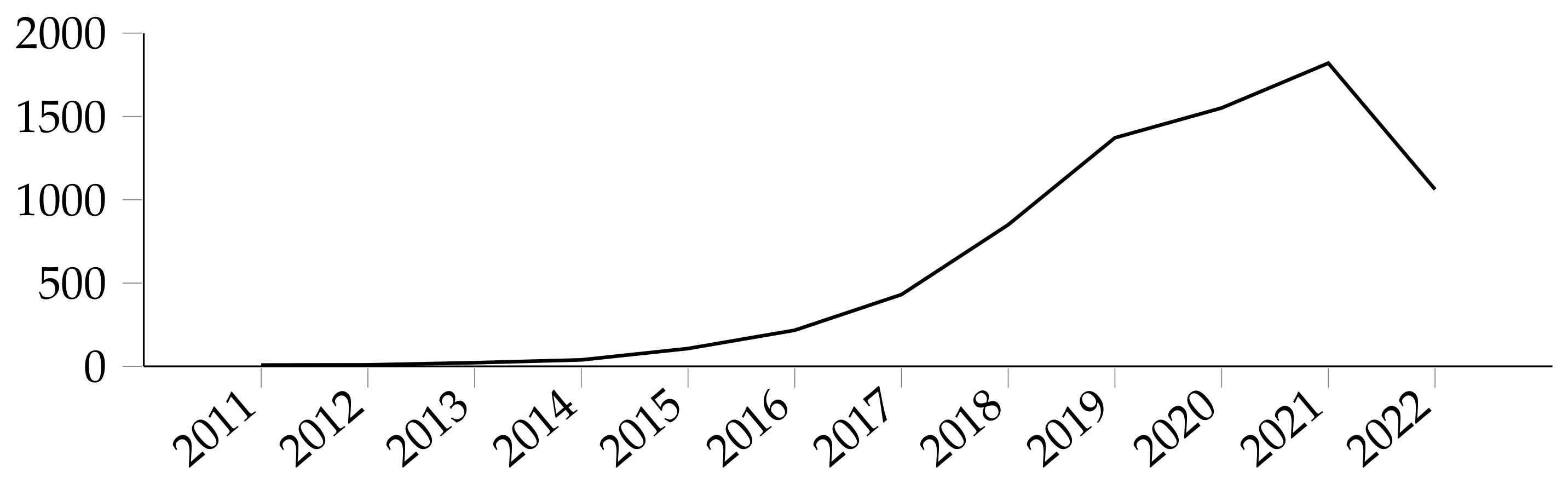
12], most pooling proposals and ideas appear to be chronologically placed in the last decade.
Figure 1 shows a steady interest in the general subject of pooling for the last decade, perhaps with small increases or decreases per year.
2.3. Let the Pooling Begin
Three of the most common pooling methods are Max pooling, Min pooling, and Average pooling. As their names suggest, for every area of the input where the sliding window focuses, the maximum, minimum, or average value is calculated accordingly.
Average pooling (also referred to as Mean pooling) has the drawback that it takes into consideration all values regardless of their magnitude, and even worse, in some cases (depending on the activation function that is used), strong positive and negative activations can cancel each other out completely.
On the other hand, Max pooling captures the strongest activations while ignoring other weaker activations that might be equally important, thus erasing input data, while also tending to overfit frequently and not generalizing very well. While most of the other methods try to either improve, combine, or even completely replace these “basics”, they still tend to be widely used due to their efficiency, ease of use, and low computational power required. Let us explore each of the available methods in detail.
2.3.1. Max and Min Pooling
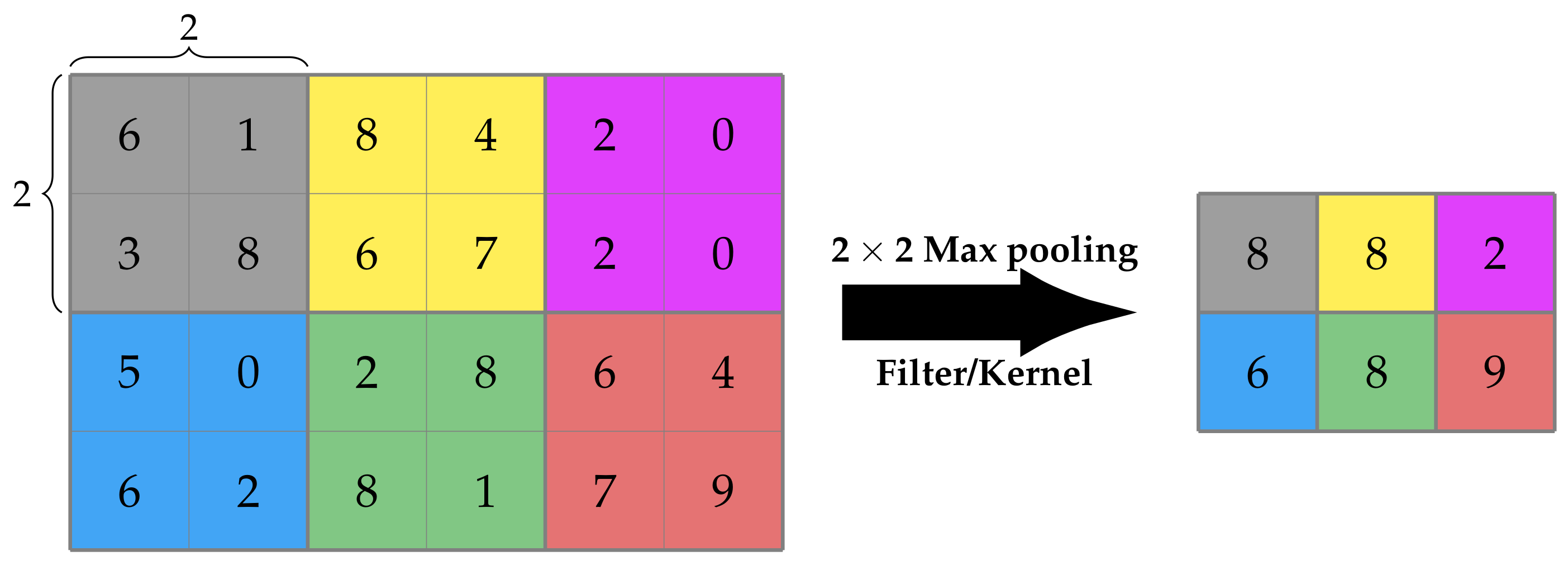
Max pooling is one of the most-common pooling methods, which selects the maximum element from the area of the feature map covered by the kernel applied, as seen in
Figure 2. Depending on the filter and stride, the outcome is a feature map having the most distinguished features of the input [
13]. On the other hand, Min pooling does the exact opposite, selecting the minimum element from the selected area. As expected, Max pooling tends to retain the lighter parts of the input when it comes to images, while Min pooling does the same with the darker parts.
2.3.2. Fractional Max Pooling
Fractional Max Pooling (FMP) [
15] is, as its name suggests, a variant of Max pooling, but the reduction ratio can be a fraction as well, instead of an integer. The most important parameter is the scaling factor
α by which the input image will be downscaled, with
. Considering an input of size
, we select two sequences of integers
,
that start at 1, and they are incremented by 1 or 2 and end at
. These sequences can be either completely random or pseudorandom when they follow the equation
, where
α is the scaling factor and
u is a number in the range (0, 1). Then, the input is split into pooling regions, either disjoint or overlapping using the respective variant of Formula (
1), and the Max value for each region is retained.
where
According to the writers’ experiments, overlapping FMP seems to have better results than the disjoint alternative, while a random choice of the sequences , distorts the image, in contrast with the pseudorandom ones. Overall, FMP’s performance appears to be better than that of Max pooling.
2.3.3. Row-Wise Max-Pooling
Row-wise Max pooling is referred to alongside a deep panoramic representation for 3D shape classification and recognition called DeepPano [
16]. A panoramic view is created from the projection of the 3D model as a cylinder to its principle axis. The pooling layer is placed after the last convolution layer and uses the highest value of each row in the input map. The suggested methodology appears to be rotation-invariant according to the experiments, since its output is not affected by the rotation of the 3D shape input.
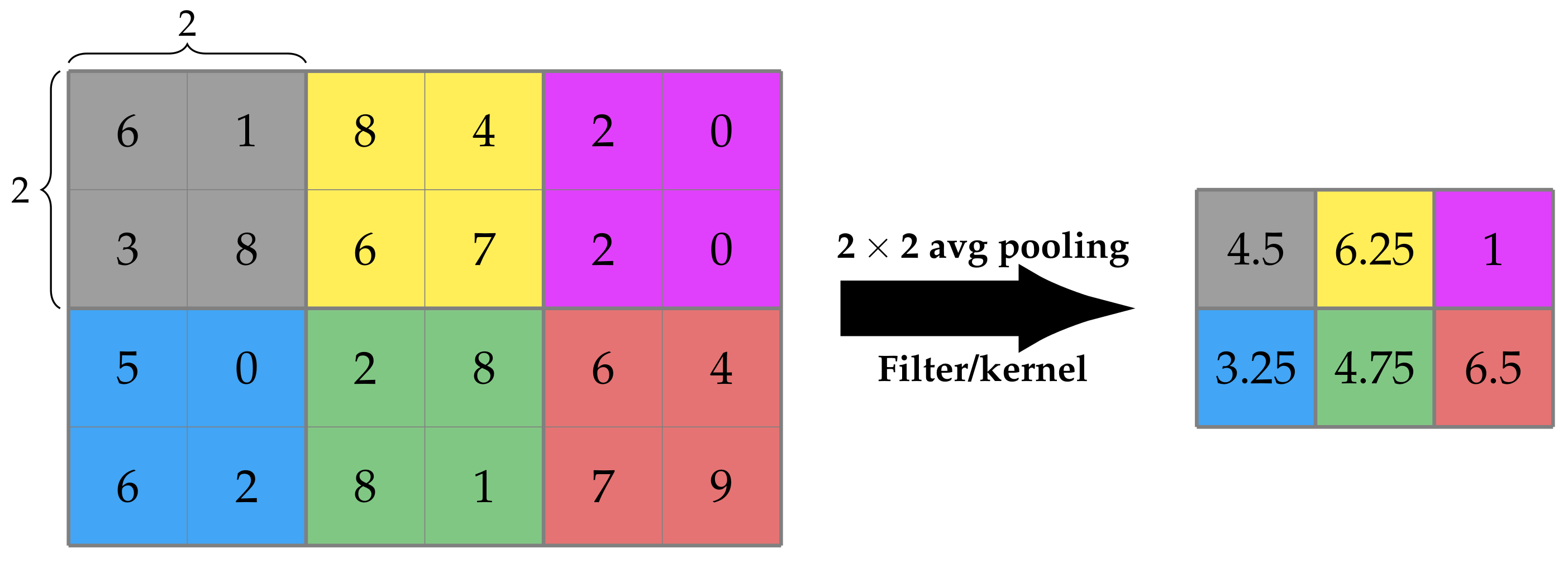
2.3.4. Average Pooling
Average pooling has a similar function as Max pooling, but it calculates the average value of the pooled area [
17], as seen in
Figure 3.
Average pooling, in contrast to Max pooling, which seeks the top features, extracts a patch of features, makes some calculations based on them, and returns a smoother result. This may lead to lower accuracy. In general, it depends on the density of the features (pixels) and the use of the output product.
2.3.5. Rank-Based Pooling
The rank-based pooling methods [
18] are an alternative to Max pooling, with three variants: rank-based Average pooling (RAP), rank-based weighted pooling (RWP), and rank-based stochastic pooling (RSP). The most-important characteristics of these methods are:
The top features can be easily identified by their ranks.
Ranks remain slightly unchanged from the activation values.
Ranking can avoid scaling across value-based methods.
Before applying any of the three methods, the ranking process takes place, where an activation function is applied to the individual elements, and they are sorted in descending order according to that function’s value.
RAP attempts to resolve the main issues of Max and Average pooling, which are the information loss of non-Max values in Max pooling and the information being downgraded due to near-zero negative activations in Average pooling. It does so by using an average of the top t important features, where
t is a predefined downsizing threshold—if we want to downsize, for instance, by a factor of 2 and the kernel has a size of 2 × 2,
t will have the value of 2 as well. Then, we set weights for all the elements within the kernel, with the top t having a weight of 1/
t, whereas all other weights are set to 0, and the output is calculated from Equation (
2).
where
a is the activation function value and
t is the rank threshold that determines which activation affects the averaging.
RWP takes into consideration that each region in an image might not be equally important, thus setting rank-based weights for each activation. Thus, the pooling output now changes to Equation (
3).
where
a is the activation value and the probability
p that is used for each weight is given by the ranking Equation (
4) where
b is a hyper-parameter,
r is the rank of activations, and
n is the size of the pooling area.
Lastly, Equation (
5) is used for RSP in a very similar way to RWP.
where
is the activation value for each element in the pooled region. Then, the final activation values are sampled based on probabilities
p calculated by a multinomial distribution, based on Formula (
4).
2.3.6. Mixed, Gated, and Tree Pooling
Mixed pooling [
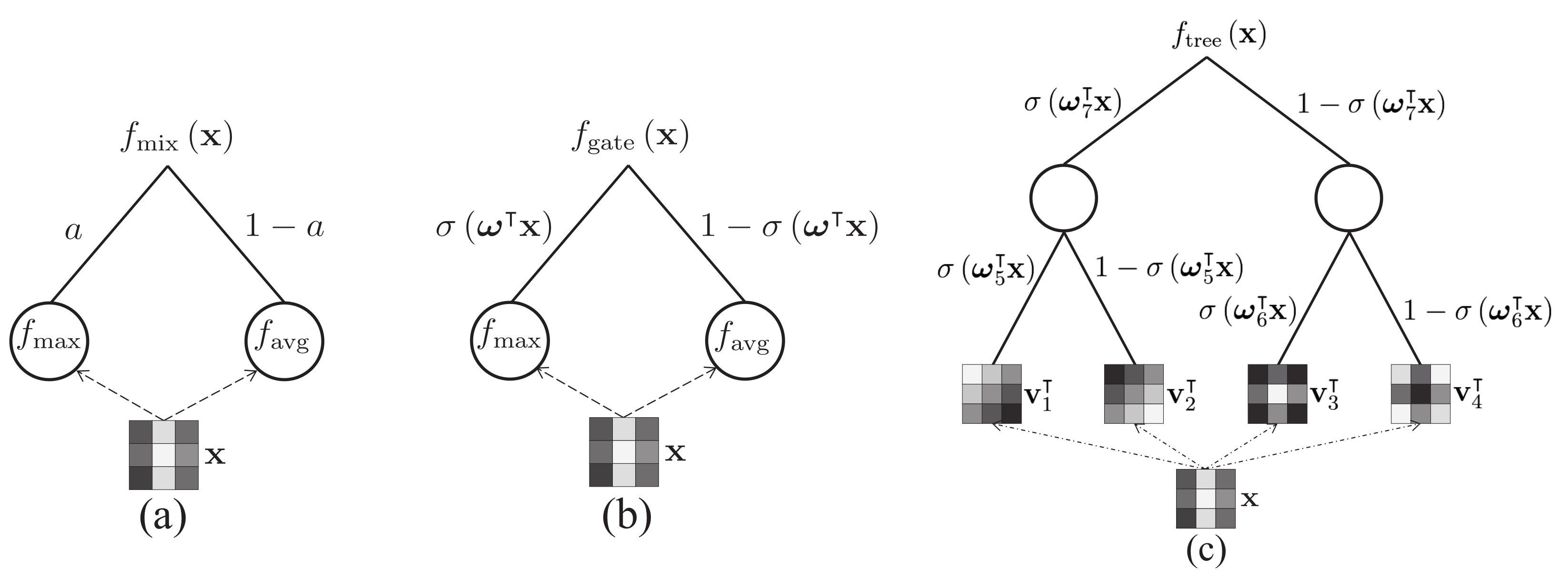
19] combines Max and Average pooling, selecting one of these two methods, outperforming both of them when used separately. Lee et al. proposed two different variants along with the base one: mixed Max–Average pooling, and gated Max–Average pooling, along with an alternative method for tree pooling. An overview of the three methods can be seen in
Figure 4.
In
mixed Max–Average pooling, a parameter
is learned and can be different per the whole network, per layer, or per pooling region. Then, the output of the pooling layer is computed by Equation (
6):
where:
In
gated Max–Average pooling, a mask of weights is learned and the inner product of that mask with the pooled region passed through a sigmoid function is used to decide whether to use Max or Average pooling. This mask can differ per network, layer, or region. The output is then calculated as described in Equation (
7). According to the method’s paper [
19], in a comparison between this method and mixed Max–Average pooling, it appears that the gated variant performs consistently better.
where:
x: the input to be pooled;
: the learned mask of weights;
T: the transpose operator;
: a sigmoid function, .
A third alternative was proposed in the same paper for
tree pooling, where a binary tree is used and the pooling filters are learned. The tree level is a pre-defined parameter, and each node holds a learned pooling filter. Furthermore, gating masks are used in a similar way as described for gated pooling previously. Thus, the pooling result for each node is described by the function (
8), and the output of the pooling method is the calculated output for the root node.
where:
: the learned filter for each node;
: the learned mask of weights;
m: the tree node index;
T: the transpose operator;
: a sigmoid function, .
2.3.7. LP Pooling
Sermanet et al. [
20] proposed LP pooling as part of an architecture to recognize house numbers. It is essentially another alternative to the Average and Max pooling methods, closer to the one or the other depending on the value of
P, a predefined parameter chosen during the setup of the layer. This method is a sort of weighted function ending up with higher weights for more important features and lower for the lesser ones, which can be applied by using Formula (
9).
where
O is the output,
I is the input, and
G is a Gaussian kernel. We should also note that when
P = 1, it is essentially Gaussian averaging, while when
P =
∞, it is similar to Max pooling. Using this type of pooling, the authors managed to achieve an average of about 4% better accuracy than Average pooling for the Street View House Numbers (SVHN) dataset
2.3.8. Weighted Pooling
Weighted pooling [
21] is a pooling strategy that aims to use the weighted average number of matches in a particular match. This is achieved by assigning different weights to different activation methods based on common information. Three main features of weighted pooling are, firstly, the amount of information of the pooling area is quantified by information theory for the first time. Second, each activation’s benefaction is quantified for the first time, and these contributions reduce the uncertainty of the pooling area in which it is placed. Last, for selecting a senator in this pooling area, the weight of each activation clearly overtakes the value of activation.
2.3.9. Stochastic Pooling
Stochastic pooling [
22] attempts to improve the commonly used Max and Average pooling and their previously mentioned drawbacks, by selecting the pooled values of the input based on probabilities. According to this suggestion, a probability
is calculated for each of the elements inside the pooling region using Formula (
10), and then, one of the elements with a probability greater than zero is chosen randomly. This method though does appear to have a drawback similar to that of Max pooling, since important parts of the input might be ignored in favor of other parts with non-zero probabilities. The stochastic pooling strategy can be joined with any other forms of regulation such as dropout, data augmentation, weight decay, and others to avoid overfitting in deep convolutional network training.
where:
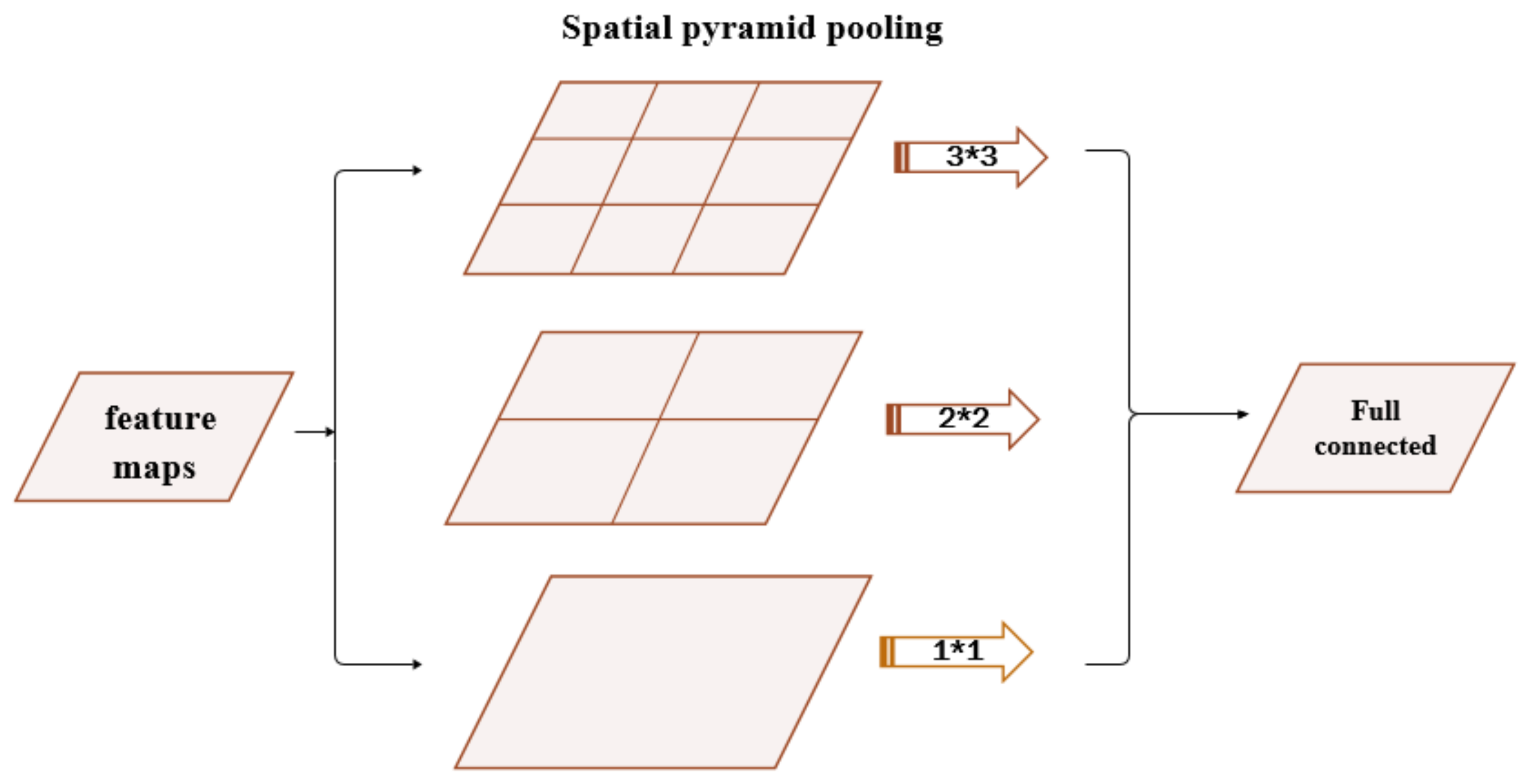
2.3.10. Spatial Pyramid Pooling
Spatial Pyramid Pooling (SPP) was inspired by the bag-of-words model [
23], which is one of the best-known representation algorithms for object categorization. The fully connected layers at the end of the CNNs require a fixed length input. Spatial pyramid pooling [
24] attempts to fix that by converting the input of any size into a predefined fixed length, essentially removing that fixed-size constraint, which might be problematic. Basically, a fixed-size window with a constant stride makes the output be relative to the input. On SPP layers the stride, and the pooling window are proportional to the input image, so the output can be a fixed size. The name came from the ability of the layers to apply more than one pooling operation and combining the outcome prior to moving on to the next layer, as described in
Figure 5.
2.3.11. Per-Pixel Pyramid Pooling
The largest pooling window used in per-pixel pyramid pooling [
26] differs from the original spatial pyramid pooling method, in order to manage obtaining the desired size of the receptive field. This may have as a result the loss of some of the finer details. For that reason, more than one pooling layer with different window sizes is applied, and the outputs are combined to create new feature maps. This pooling task is executed for every pixel without strides. The output is calculated by Equation (
11).
where
s is a vector with M elements,
F is the pooling function applied, and
P(
F,
si) is the pooling operation with an s
i-sized kernel and stride 1.
2.3.12. Fuzzy Pooling
The Type-1 fuzzy pooling [
27] is achieved by combining the fuzzification, aggregation, and defuzzification of feature map neighborhoods. The method is applied using the following steps:
The input of depth n is sampled with a kernel of size k × k and a specific stride to obtain a set of patches p.
For each patch, we apply a set of membership functions , obtaining a set of fuzzy patches .
Each fuzzy patch is summed, resulting in a sum .
For each patch, the fuzzy patch with the highest sum of the previous step is selected out of the total set of fuzzy patches ().
Finally, the dimensionality is reduced using Equation (
12):
2.3.13. Overlapping Pooling
Overlapping pooling was proposed as part of a paper with the suggestion of an architecture that classifies the ImageNet LSVRC-2010 dataset [
28]. The idea behind it that can be applied to most—if not all—pooling methods is setting a smaller stride than the kernel size, so that there is overlap between neighboring pooled regions. The experiments with the proposed architecture showed that the top 1 and top 5 error rates were reduced by 0.4% and 0.3%, respectively for the case of Max pooling, while the model seemed to overfit slightly less when using overlapping—while that was rather an observation, and no specific evidence was presented.
2.3.14. Superpixel Pooling
Superpixel is a term for 2D image segments. Essentially, superpixel pooling [
29], just like overlapping pooling, is not a pooling method itself, but a method of applying a pooling function such as the Max or Average. The difference is that, instead of using a standard square sliding kernel as in other methods, the 2D image is already segmented—usually based on edges. Then, the selected pooling function is applied in each segment. This process reduces the computational cost significantly, while preserving a high accuracy in the models used.
2.3.15. Spectral Pooling
While most other methods process the input in the spatial domain, spectral pooling [
30] takes it to the frequency domain, pools the input, and then, returns the output back to the spatial domain. One of the main advantages is that information is preserved better—compared to other common methods such as Max pooling—since lower frequencies tend to contain that information and higher frequencies usually contain noise.
The application of this type of pooling is rather straightforward, applying a Discrete Fourier Transform (DFT) to the input, cropping a predefined size window from the center, and returning it back to the spatial domain by using the inverse DFT.
Obviously, a significant issue is the computational cost, since the DFT is required—both forward and inverse. That overhead though can be minimized when the FFT is used for the calculation of the convolution in the previous layer, thus limiting its use only to such scenarios. Zhang et al. [
31] suggested an alternative implementation based on the Hartley transform, which might require less computational power while retaining the same amount of information.
2.3.16. Wavelet Pooling
The wavelet pooling method [
32] features a completely different approach compared to the previously mentioned ones that use neighboring inputs, attempting to minimize the artifacts produced during the process of pooling. It is based on the Fast Wavelet Transform (FWT), a transformation that is applied twice on the input, once on the rows, and once again on the columns. Then, the input features are reconstructed using only the second-order wavelet sub-bands by applying the Inverse FWT (IFWT), reducing by half the total image features.
Unfortunately, though on the MNIST dataset, the wavelet pooling managed to outperform other competitors, on other datasets (CFAR-10, SHVN, KDEF), simpler methods such as Average or Max pooling performed better. Furthermore, as one can see in
Table 1, the computational power required appears to be 110 K mathematical operations for the simpler MNIST dataset, which goes up to a tremendous total of 6.2 M for the KDEF dataset, compared to 3.5 K and 29 K—200-times less—operations required by the much simpler-to-apply Average pooling.
2.3.17. Intermap Pooling
To achieve an increase in robustness for spectral variations of audio signals and acoustic features, Intermap Pooling (IMP) was introduced [
33]. This was accomplished by the addition of a convolution maxout layer (IMP), which groups the feature maps, and then the Max activation function at each position is chosen.
2.3.18. Strided Convolution Pooling
Ayachi et al. [
34] proposed strided convolution as a drop-in replacement for Max pooling layers with the same stride and kernel size, attempting to make the CNNs more memory efficient. The convolution function that is applied is:
where
is the activation function,
[0,
m] is the total number of output feature maps of the previous convolution layer,
k is the kernel size,
are the width, height, and number of channels, and finally,
is the kernel of the convolution weights, and it is
if
, or
otherwise.
In
Table 2, one can easily see that the replacement of the pooling layer with the strided convolution does seem promising, since it actually reduces the total memory required by each model while also increasing the overall accuracy.
2.3.19. Center Pooling
Center pooling [
35] is a pooling method used for object detection and intends to identify distinct and more recognizable visual patterns. In an output feature map, we obtain the maximum values for a pixel in it is vertical and horizontal axis and add them—which will show us if that pixel is a center keypoint, which is the center of a detected object within an image.
2.3.20. Corner Pooling
On the other hand, corners usually are located outside the objects, which do not have local relative features. Therefore, corner pooling [
36] was introduced to solve this problem. Corner pooling finds the maximum values on the boundary directions and, in this way, identifies the corners. This has an effect on making the corners sensitiveto the edges. Addressing this issue, in order to let corners identify the visual patterns of the objects if needed, we use the cascade corner pooling method. Detecting the corners of an object can help define the edges of an object itself better.
2.3.21. Cascade Corner Pooling
Cascade corner pooling [
37] looks like a combination of center and corner pooling, by taking the maximum values in both the boundary directions and internal directions of the objects. Initially, from each boundary, it finds a boundary maximum value, then proceeds to look inside the location of the boundary maximum value to obtain an internal maximum value, and finally, it adds them together. As a result, the corners obtain both the boundary information and the visual patterns of objects.
2.3.22. Adaptive Feature Pooling
Adaptive feature pooling [
38] is used to gather features from all layers for each object detection proposition and merges them for the upcoming prediction. For each one, they are mapped at other feature levels. It is usually used to pool grids of features from each level. A fusion function (maximum or sum of elements) is then used to secure the grids of features from different levels.
2.3.23. Local-Importance-Based Pooling
Local-Importance-based Pooling (LIP) [
39] is a pooling layer that can increase discreet features during the downsampling process by learning adaptive weightings based on inputs. Using this kind of didactic network, the importance function now is not limited to manual forms and has the ability to recognize the criterion for the discriminativeness of features. Furthermore, the size of the LIP window is limited to a minimum dimension, so that it is not less than the step of making full use of the feature map and avoiding the issue of a defined sampling interval. More specifically, the importance function in LIP is implemented by a tiny fully convergent network, which learns to generate the importance map based on end-to-end inputs [
40].
2.3.24. Soft Pooling
Soft Pooling (SoftPool) [
41] is a quick and effective kernel-based process that aggregates exponentially weighted activations, as described in Formula (
14). In comparison with a number of other methods, SoftPool holds more information in the downsampled activation maps, so by having a more sophisticated downsampling process, the result returns better classification accuracy. It can be used to downsample 2D images and 3D video activation maps.
where:
3. Putting the Methods to the Test
3.1. The Benchmark Setup
In order to choose the optimal architecture and datasets to use for our benchmark,
Table 3 was compiled. which summarizes what was used for each method in the corresponding paper.
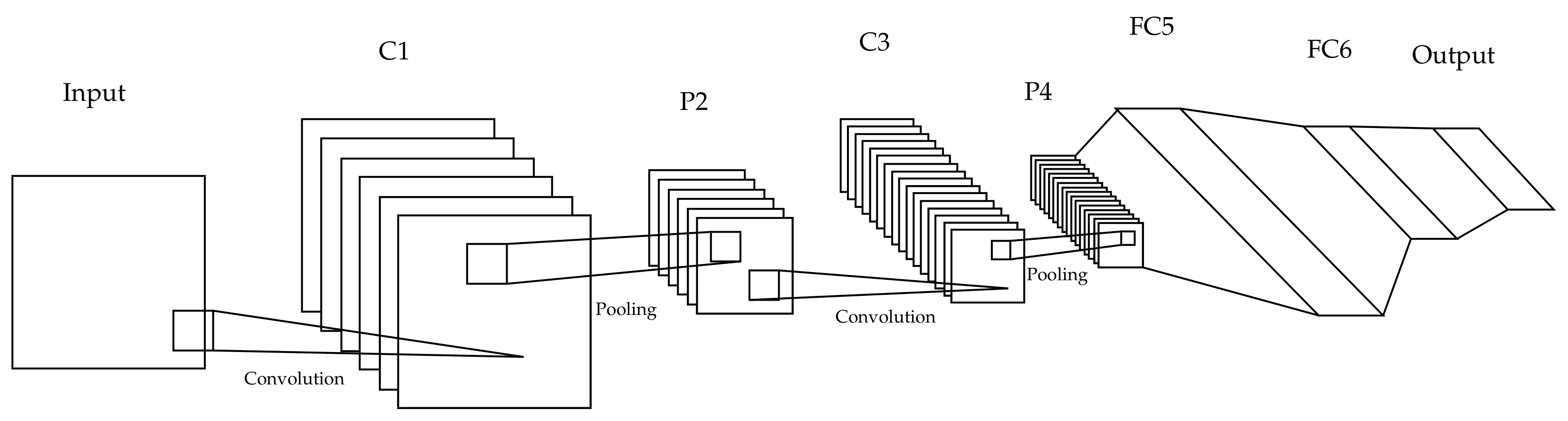
It seems that less-potent architectures are preferred in most cases. This is probably because they usually achieve a lower overall performance, but that also means that the impact of changing the pooling layer will be better highlighted. Thus, a similar model was chosen, a LeNet5 architecture with 2 convolution layers, 2 respective interchangeable pooling layers, and 2 fully connected layers, as shown in
Figure 6.
Regarding the datasets, the MNIST, CIFAR10, and CIFAR100 were used, since it seems from
Table 3 that these are commonly used in the reviewed papers. They are also ideal since we had to make sure they were interchangeable for the exact same architecture without changes to the fully connected layer(s), just by modifying the total output class parameter.
Lastly, we focused on testing pooling methods that can be used as a direct drop-in replacement for the Max pooling layer, with a kernel size and stride of size 2, in order to reduce each dimension by half—applying parameters that would provide similar results wherever required (like a 0.5 scaling factor, for instance, for the spectral pooling layer). Stochastic gradient descent was used as an optimizer, with a learning rate of 0.01 and momentum of 0.9 over 300 epochs.
3.2. Performance Evaluation
For the performance comparison, we used the standard top 1 and top 5 testing accuracy (higher is better); for the computational complexity, we used the time required per epoch (lower is better), while also including three indicators, which can provide better insight into how well the details of the original image are maintained—for all three (higher values are better):
Root-Mean-Squared Contrast (RMSC) [
44], as defined in Formula (
15) for a
image:
where
Peak-Noise-to-Signal Ratio (PSNR) [
45], as defined in Formula (
16) for a
image:
where:
Structural Similarity Index (SSIM) [
46], which is defined by three combined metrics for luminance, contrast, and structure and can be simplified for two signals
in the form seen in Formula (
17):
where:
All tests were performed using a PyTorch implementation of the methods, on an Nvidia GTX1080 GPU.
4. Results
4.1. Details Retention
As previously described, three metrics were used as a means of comparison for how well details are preserved after pooling the original input. The first one is the Root-Mean-Squared Contrast (RMSC) [
44], which is the standard deviation of the pixel intensities, which indicates how well the contrast levels are maintained between the input and output. The second, the Peak-Noise-to-Signal Ratio (PSNR) [
45], shows how strong the original image signal is compared to the introduced noise due to pooling. Lastly, the Structural Similarity Index (SSIM) [
46] can range from −1 to 1 and shows the actual similarity between the input and output of the pooling layer.
In
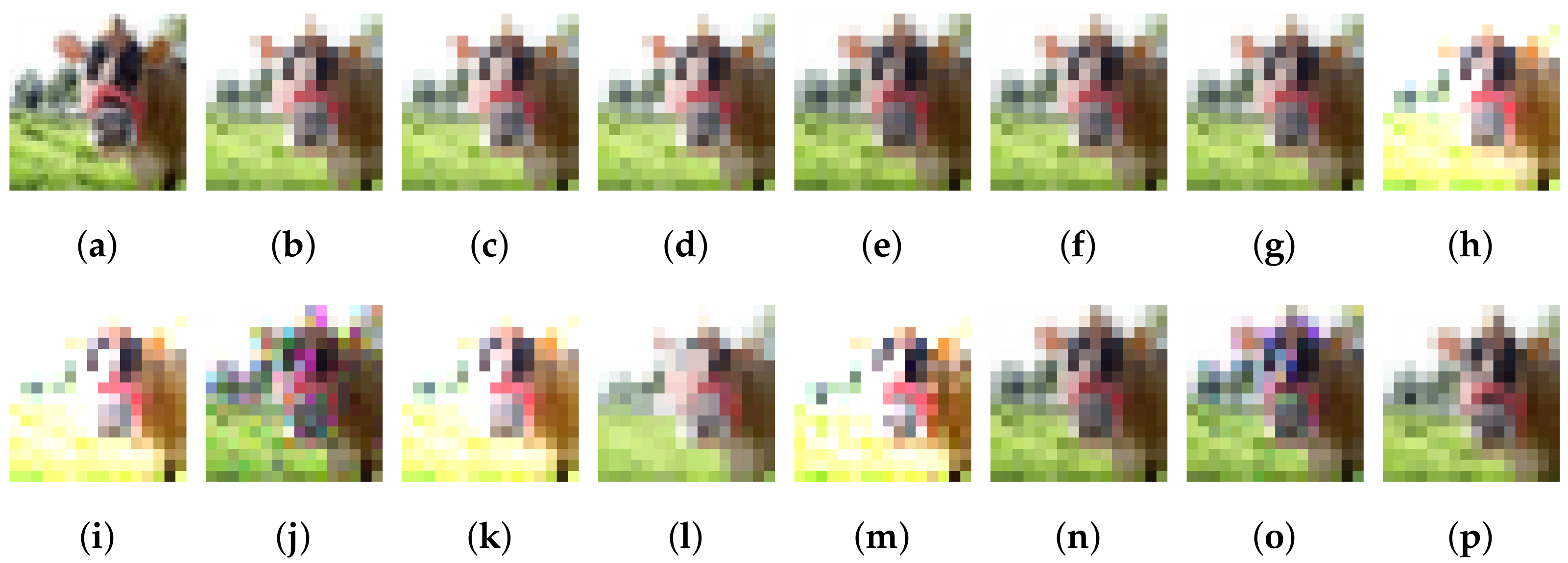
Table 4, Average pooling appears to be the best choice, since it shows the best SSIM values across all dataset tests. Furthermore, it achieved a top ranking PSNR as well for two out of the three datasets—which can be interpreted as a low level of introduced noise. When it comes to the RMSC, though other methods achieved better values, Average pooling kept up, and as we can see in the pooling layers’ output examples, higher contrast is not always good, at least when it comes to comparing similarities with the original image.
In
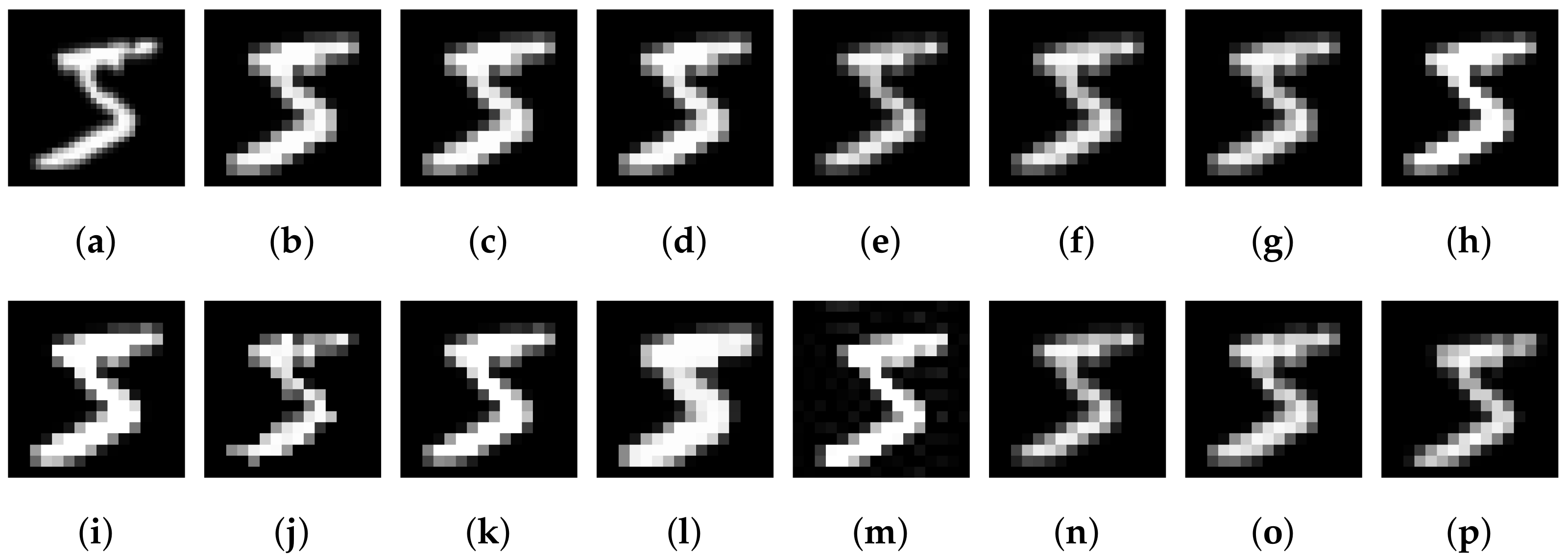
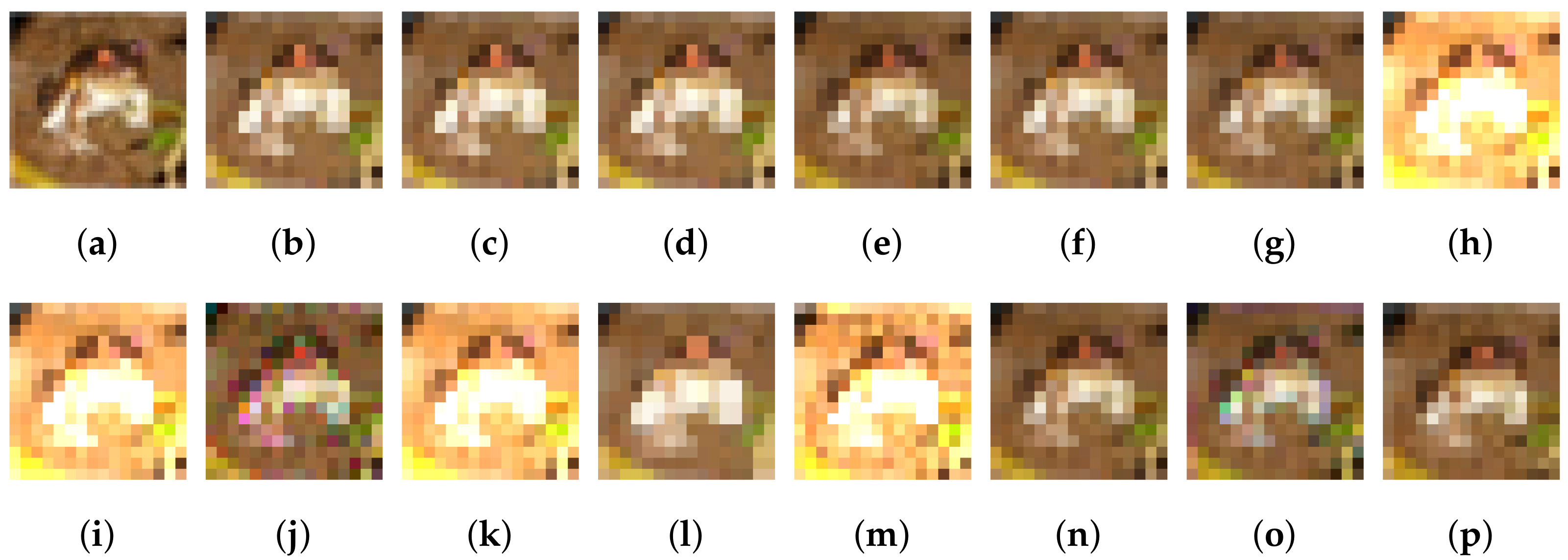
Figure 7,
Figure 8 and
Figure 9, a sample input of each dataset is presented, as well as the respective output for each pooling layer. Each method might have a tendency to favor higher or lower values of the input pixels, while some increase the contrast significantly.
Combined with the results of
Table 4, it seems that Average pooling indeed achieved a result that was very close to the original image. On the other hand, tree, l2, fuzzy, and spectral pooling introduced a much higher contrast to the image, generating an output that was very different from the original input.
4.2. Model Performance
In
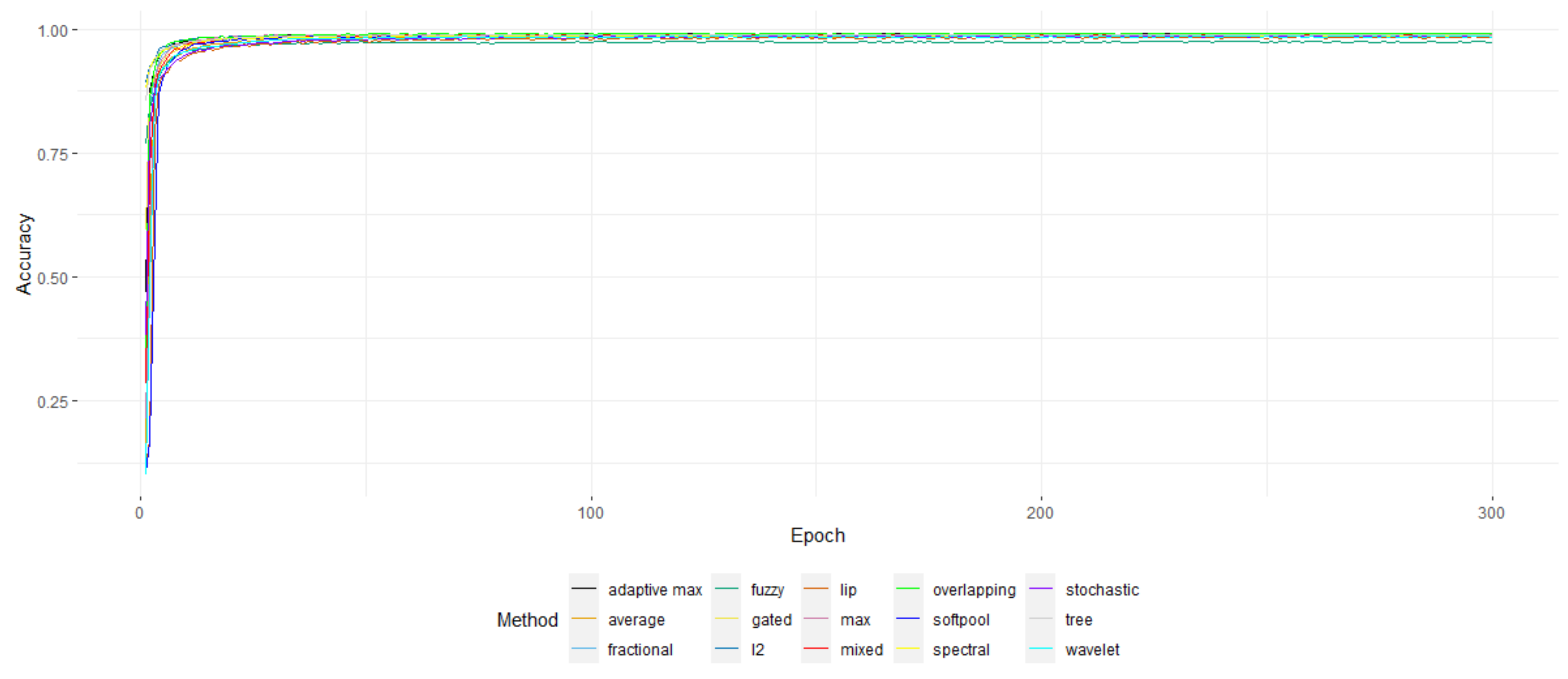
Table 5, the accuracy of the individual pooling methods is presented, along with the time required per epoch. It appears that for the MNIST, perhaps due to the ease of the dataset, the results were almost identical. Though, in the previous section, Average pooling appeared to “win the battle” of details’ retention, here, it is obvious that Max pooling and its variants—especially overlapping Max pooling—seemed to perform much better.
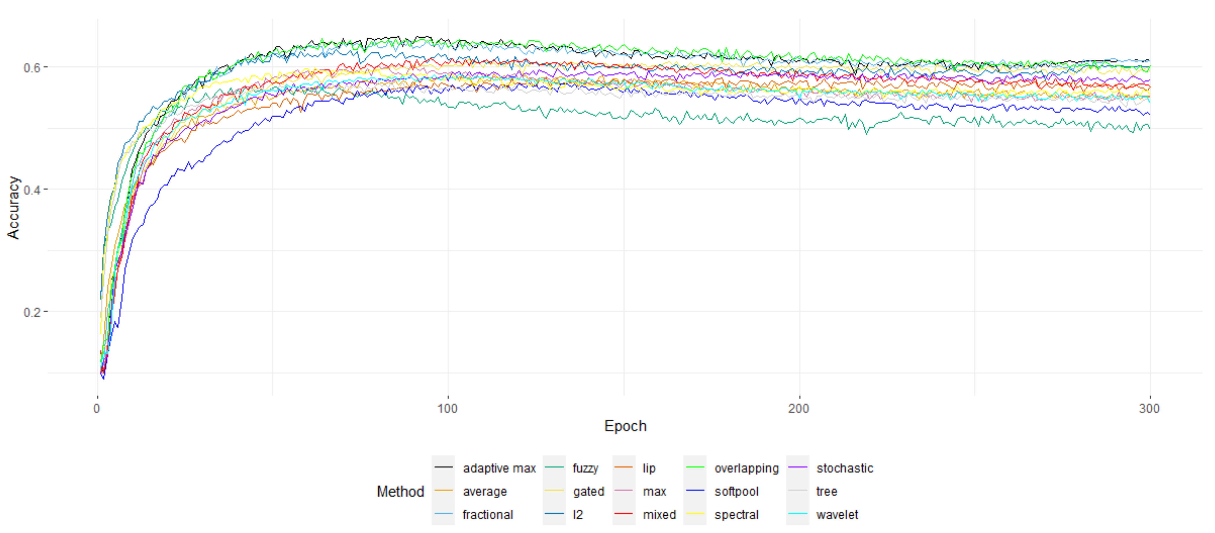
Figure 10,
Figure 11 and
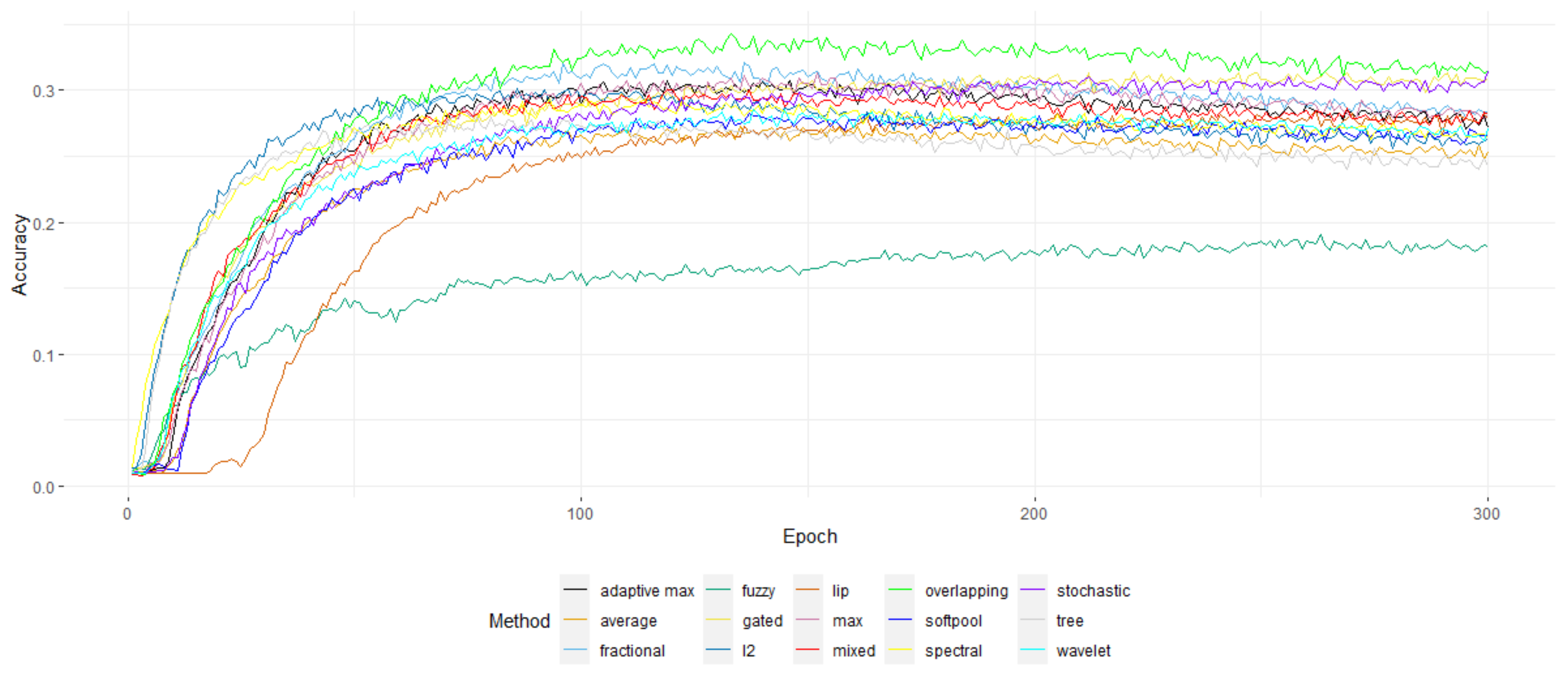
Figure 12 show the top 1 accuracy of the model over the 300 training epochs of the benchmark. In
Figure 12, it is clear that overlapping Max pooling is the overall better-performing method for CIFAR100, significantly outperforming the rest—though the difference is not that obvious for the other two datasets.
When it comes to complexity, most methods required about 8 s per epoch, with some requiring a much increased time—which might perhaps perform much better with a C++ implementation. Overlapping Max pooling had one of the lowest times required per epoch, giving it yet another advantage. On the other hand, some methods managed to converge much more quickly. For instance, tree, l2, spectral, and Average pooling seemed to require far less than 100 epochs to obtain the highest possible accuracy. Thus, l2 might be a better choice after all, since it achieved a high accuracy in fewer epochs and one of the lowest processing times per epoch.
On a closing note, the overall selected amount of 300 epochs might be a bit higher than required since most methods achieved their peak accuracy at less than 100–150 epochs. The high amount of epochs though did make sure that there were enough for each method to achieve the best performance possible.
5. Discussion
As expected, there is no “absolute best” for the pooling layer—one that may work great for one application might not even be viable for another. Though overlapping Max pooling seemed to be the “winner” of this benchmark, there may be different scenarios where other commonly used methods may be more suitable—such as, for instance, when detail retention is important, Average pooling is a better choice and easy to implement and has similar performance. Therefore, the choice of the proper pooling layer is not always that simple and straightforward.
One of the most important factors is probably the overall computational power required. Since the convolution layer itself is resource-heavy and the pooling layer’s role is to “relieve” part of that load, it would be expected for the added overhead to be as minimal as possible.
Other factors that one should keep in mind are the level of invariance required—usually when the input is a video or highly variable images of similar objects—and the overall detail retention that is required. Of course, a combination of two or even more pooling methods could be applied to further improve the overall accuracy of the output. Some might even prefer simpler methods due to their ease of implementation—in the case where a rapid prototype would be adequate as a proof of concept. Taking into consideration all the model’s requirements and even the personal favorites of the development team is what usually drives the final selection of the pooling layer.
6. Conclusions
CNNs are an important part of computer vision, and pooling can significantly reduce their overall processing, allowing the implementation of models and architectures with far fewer resources than would normally be required. We created a roundup of many of the pooling methods that have been proposed so far—though it might not be exhaustive—summarizing each approach and a benchmark for a practical comparison.
Overlapping Max pooling appeared to perform better than the rest, at least for the selected datasets. Even though it might be next to impossible to pinpoint and test every single variation for all existing pooling methods, hopefully, it will be more than enough to function as a starting point for every researcher and machine learning scientist in order to help choose the one that is more appropriate or even inspire new approaches or improvements for current implementations.
Author Contributions
Conceptualization, G.A.P.; methodology, N.-I.G., P.V. and K.-G.M.; software N.-I.G., P.V. and K.-G.M.; validation N.-I.G.; formal analysis, N.-I.G., P.V. and K.-G.M.; investigation, N.-I.G., P.V. and K.-G.M.; resources, N.-I.G., P.V. and K.-G.M.; data curation, N.-I.G.; writing—original draft preparation, N.-I.G., P.V. and K.-G.M.; writing—review and editing, N.-I.G.; visualization, N.-I.G., P.V.; supervision, G.A.P.; project administration, N.-I.G.; funding acquisition, G.A.P.; All authors have read and agreed to the published version of the manuscript.
Funding
This research received no external funding.
Data Availability Statement
Acknowledgments
This work was supported by the MPhil program “Advanced Technologies in Informatics and Computers”, hosted by the Department of Computer Science, International Hellenic University, Kavala, Greece.
Conflicts of Interest
The authors declare no conflict of interest.
References
- Forsyth, D.A.; Ponce, J. Computer Vision: A Modern Approach; Prentice Hall: Upper Saddle River, NJ, USA, 2002. [Google Scholar]
- Carandini, M. What simple and complex cells compute. J. Physiol. 2006, 577, 463–466. [Google Scholar] [CrossRef]
- Movshon, J.A.; Thompson, I.D.; Tolhurst, D.J. Spatial summation in the receptive fields of simple cells in the cat’s striate cortex. J. Physiol. 1978, 283, 53–77. [Google Scholar] [CrossRef] [PubMed]
- Fukushima, K.; Miyake, S. Neocognitron: A self-organizing neural network model for a mechanism of visual pattern recognition. In Competition and Cooperation in Neural Nets; Springer: Berlin/Heidelberg, Germany, 1982; pp. 267–285. [Google Scholar]
- Lin, Y.; Lv, F.; Zhu, S.; Yang, M.; Cour, T.; Yu, K.; Cao, L.; Huang, T. Large-scale image classification: Fast feature extraction and svm training. In Proceedings of the CVPR 2011, Colorado Springs, CO, USA, 20–25 June 2011; pp. 1689–1696. [Google Scholar]
- Zhang, H.; Berg, A.C.; Maire, M.; Malik, J. SVM-KNN: Discriminative nearest neighbor classification for visual category recognition. In Proceedings of the 2006 IEEE Computer Society Conference on Computer Vision and Pattern Recognition (CVPR’06), New York, NY, USA, 17–22 June 2006; Volume 2, pp. 2126–2136. [Google Scholar]
- Akhtar, N.; Ragavendran, U. Interpretation of intelligence in CNN-pooling processes: A methodological survey. Neural Comput. Appl. 2020, 32, 879–898. [Google Scholar] [CrossRef]
- Sharma, S.; Mehra, R. Implications of pooling strategies in convolutional neural networks: A deep insight. Found. Comput. Decis. Sci. 2019, 44, 303–330. [Google Scholar] [CrossRef]
- Khan, A.; Sohail, A.; Zahoora, U.; Qureshi, A.S. A survey of the recent architectures of deep convolutional neural networks. Artif. Intell. Rev. 2020, 53, 5455–5516. [Google Scholar] [CrossRef]
- Gholamalinezhad, H.; Khosravi, H. Pooling Methods in Deep Neural Networks, a Review. arXiv 2020, arXiv:2009.07485. [Google Scholar]
- Nirthika, R.; Manivannan, S.; Ramanan, A.; Wang, R. Pooling in convolutional neural networks for medical image analysis: A survey and an empirical study. Neural Comput. Appl. 2022, 34, 5321–5347. [Google Scholar] [CrossRef] [PubMed]
- Yamaguchi, K.; Sakamoto, K.; Akabane, T.; Fujimoto, Y. A neural network for speaker-independent isolated word recognition. In Proceedings of the First International Conference on Spoken Language Processing, Kobe, Japan, 18–22 November 1990. [Google Scholar]
- Murray, N.; Perronnin, F. Generalized Max pooling. In Proceedings of the IEEE Conference on Computer Vision and Pattern Recognition, Columbus, OH, USA, 23–28 June 2014; pp. 2473–2480. [Google Scholar]
- Thoma, M. LaTeX Examples. 2012. Available online: https://github.com/MartinThoma/LaTeX-examples (accessed on 8 September 2022).
- Graham, B. Fractional Max-pooling. arXiv 2014, arXiv:1412.6071. [Google Scholar]
- Shi, B.; Bai, S.; Zhou, Z.; Bai, X. Deeppano: Deep panoramic representation for 3-d shape recognition. IEEE Signal Process. Lett. 2015, 22, 2339–2343. [Google Scholar] [CrossRef]
- Zubair, S.; Yan, F.; Wang, W. Dictionary learning based sparse coefficients for audio classification with Max and Average pooling. Digit. Signal Process. 2013, 23, 960–970. [Google Scholar]
- Shi, Z.; Ye, Y.; Wu, Y. Rank-based pooling for deep convolutional neural networks. Neural Netw. 2016, 83, 21–31. [Google Scholar] [CrossRef] [PubMed]
- Lee, C.Y.; Gallagher, P.W.; Tu, Z. Generalizing pooling functions in convolutional neural networks: Mixed, gated, and tree. In Proceedings of the Artificial Intelligence and Statistics, Cadiz, Spain, 9–11 May 2016; pp. 464–472. [Google Scholar]
- Sermanet, P.; Chintala, S.; LeCun, Y. Convolutional neural networks applied to house numbers digit classification. In Proceedings of the 21st International Conference on Pattern Recognition (ICPR2012), Tsukuba, Japan, 11–15 November 2012; pp. 3288–3291. [Google Scholar]
- Zhu, X.; Meng, Q.; Ding, B.; Gu, L.; Yang, Y. Weighted pooling for image recognition of deep convolutional neural networks. Clust. Comput. 2019, 22, 9371–9383. [Google Scholar] [CrossRef]
- Zeiler, M.D.; Fergus, R. Stochastic pooling for regularization of deep convolutional neural networks. arXiv 2013, arXiv:1301.3557. [Google Scholar]
- Zhang, Y.; Jin, R.; Zhou, Z.H. Understanding bag-of-words model: A statistical framework. Int. J. Mach. Learn. Cybern. 2010, 1, 43–52. [Google Scholar] [CrossRef]
- He, K.; Zhang, X.; Ren, S.; Sun, J. Spatial pyramid pooling in deep convolutional networks for visual recognition. IEEE Trans. Pattern Anal. Mach. Intell. 2015, 37, 1904–1916. [Google Scholar] [CrossRef] [PubMed]
- ResearchGate. Available online: https://tinyurl.com/researchgateSPPfigure (accessed on 14 May 2021).
- Park, H.; Lee, K.M. Look wider to match image patches with convolutional neural networks. IEEE Signal Process. Lett. 2016, 24, 1788–1792. [Google Scholar] [CrossRef]
- Diamantis, D.; Iakovidis, D. Fuzzy Pooling. IEEE Trans. Fuzzy Syst. 2020, 29, 3481–3488. [Google Scholar] [CrossRef]
- Krizhevsky, A.; Sutskever, I.; Hinton, G.E. ImageNet classification with deep convolutional neural networks. Commun. ACM 2017, 60, 84–90. [Google Scholar] [CrossRef]
- Schuurmans, M.; Berman, M.; Blaschko, M.B. Efficient semantic image segmentation with superpixel pooling. arXiv 2018, arXiv:cs.CV/1806.02705. [Google Scholar]
- Rippel, O.; Snoek, J.; Adams, R.P. Spectral representations for convolutional neural networks. arXiv 2015, arXiv:1506.03767. [Google Scholar]
- Zhang, H.; Ma, J. Hartley Spectral Pooling for Deep Learning. arXiv 2018, arXiv:1810.04028. [Google Scholar]
- Williams, T.; Li, R. Wavelet pooling for convolutional neural networks. In Proceedings of the International Conference on Learning Representations, Vancouver, BC, Canada, 30 April–3 May 2018. [Google Scholar]
- Lee, H.; Kim, G.; Kim, H.G.; Oh, S.H.; Lee, S.Y. Deep CNNs Along the Time Axis with Intermap Pooling for Robustness to Spectral Variations. IEEE Signal Process. Lett. 2016, 23, 1310–1314. [Google Scholar] [CrossRef]
- Ayachi, R.; Afif, M.; Said, Y.; Atri, M. Strided convolution instead of Max pooling for memory efficiency of convolutional neural networks. In Proceedings of the International Conference on the Sciences of Electronics, Technologies of Information and Telecommunications, Genoa, Italy and Hammammet, Tunisia, 18–20 December 2018; Springer: Berlin/Heidelberg, Germany, 2018; pp. 234–243. [Google Scholar]
- Duan, K.; Bai, S.; Xie, L.; Qi, H.; Huang, Q.; Tian, Q. Centernet: Keypoint triplets for object detection. In Proceedings of the IEEE/CVF International Conference on Computer Vision, Seoul, Korea, 27 October–2 November 2019; pp. 6569–6578. [Google Scholar]
- Law, H.; Deng, J. Cornernet: Detecting objects as paired keypoints. In Proceedings of the European Conference on Computer Vision (ECCV), Munich, Germany, 8–14 September 2018; pp. 734–750. [Google Scholar]
- Wang, J.; Sun, K.; Cheng, T.; Jiang, B.; Deng, C.; Zhao, Y.; Liu, D.; Mu, Y.; Tan, M.; Wang, X.; et al. Deep high-resolution representation learning for visual recognition. IEEE Trans. Pattern Anal. Mach. Intell. 2020, 43, 3349–3364. [Google Scholar] [CrossRef] [PubMed]
- Liu, S.; Qi, L.; Qin, H.; Shi, J.; Jia, J. Path aggregation network for instance segmentation. In Proceedings of the IEEE Conference on Computer Vision and Pattern Recognition, Salt Lake City, UT, USA, 18–22 June 2018; pp. 8759–8768. [Google Scholar]
- Gao, Z.; Wang, L.; Wu, G. Lip: Local importance-based pooling. In Proceedings of the IEEE/CVF International Conference on Computer Vision, Seoul, Korea, 27 October–2 November 2019; pp. 3355–3364. [Google Scholar]
- Hyun, J.; Seong, H.; Kim, E. Universal pooling—A new pooling method for convolutional neural networks. Expert Syst. Appl. 2021, 180, 115084. [Google Scholar] [CrossRef]
- Stergiou, A.; Poppe, R.; Kalliatakis, G. Refining activation downsampling with SoftPool. arXiv 2021, arXiv:2101.00440. [Google Scholar]
- Scharstein, D.; Szeliski, R. A taxonomy and evaluation of dense two-frame stereo correspondence algorithms. Int. J. Comput. Vis. 2002, 47, 7–42. [Google Scholar] [CrossRef]
- Vedaldi, A.; Lenc, K. Matconvnet: Convolutional neural networks for matlab. In Proceedings of the 23rd ACM International Conference on Multimedia, Brisbane, Australia, 26–30 October 2015; pp. 689–692. [Google Scholar]
- Peli, E. Contrast in complex images. JOSA A 1990, 7, 2032–2040. [Google Scholar] [CrossRef]
- Instruments, N. Peak Signal-To-Noise Ratio as an Image Quality Metric. 2013. Available online: https://www.ni.com/en-us/innovations/white-papers/11/peak-signal-to-noise-ratio-as-an-image-quality-metric.html (accessed on 8 September 2022).
- Wang, Z.; Bovik, A.C.; Sheikh, H.R.; Simoncelli, E.P. Image quality assessment: From error visibility to structural similarity. IEEE Trans. Image Process. 2004, 13, 600–612. [Google Scholar] [CrossRef]
Figure 1.
Publications for total results about pooling for CNNs in Scopus.
Figure 1.
Publications for total results about pooling for CNNs in Scopus.
Figure 2.
An example of Max pooling’s functionality [
14].
Figure 2.
An example of Max pooling’s functionality [
14].
Figure 3.
An example of Average pooling’s functionality [
14].
Figure 3.
An example of Average pooling’s functionality [
14].
Figure 4.
A schematic comparison of the three proposed operations in [
19]: (
a) mixed Max–Average pooling, (
b) gated Max–Average pooling and (
c) tree pooling with 3-level binary tree.
Figure 4.
A schematic comparison of the three proposed operations in [
19]: (
a) mixed Max–Average pooling, (
b) gated Max–Average pooling and (
c) tree pooling with 3-level binary tree.
Figure 5.
A network structure with a spatial pyramid pooling layer [
25].
Figure 5.
A network structure with a spatial pyramid pooling layer [
25].
Figure 6.
The CNN architecture used for the tests.
Figure 6.
The CNN architecture used for the tests.
Figure 7.
The MNIST “5” original image (a) and the respective results of the first pass of pooling for the methods Max (b), adaptive Max (c), fractional (d), Average (e), mixed (f), gated (g), tree (h), l2 (i), stochastic (j), fuzzy (k), overlapping Max (l), spectral (m), wavelet (n), LIP (o), and SoftPool (p).
Figure 8.
The CIFAR10 frog original image (a) and the respective results of the first pass of pooling for the methods Max (b), adaptive Max (c), fractional (d), Average (e), mixed (f), gated (g), tree (h), l2 (i), stochastic (j), fuzzy (k), overlapping Max (l), spectral (m), wavelet (n), LIP (o), and SoftPool (p).
Figure 9.
The CIFAR100 horse original image (a) and the respective results of the first pass of pooling for the methods Max (b), adaptive Max (c), fractional (d), Average (e), mixed (f), gated (g), tree (h), l2 (i), stochastic (j), fuzzy (k), overlapping Max (l), spectral (m), wavelet (n), LIP (o) and SoftPool (p).
Figure 10.
The top 1 accuracy of the models for the MNIST dataset over the epochs.
Figure 10.
The top 1 accuracy of the models for the MNIST dataset over the epochs.
Figure 11.
The top 1 accuracy of the models for the CIFAR10 dataset over the epochs.
Figure 11.
The top 1 accuracy of the models for the CIFAR10 dataset over the epochs.
Figure 12.
The top 1 accuracy of the models for the CIFAR100 dataset over the epochs.
Figure 12.
The top 1 accuracy of the models for the CIFAR100 dataset over the epochs.
Table 1.
A comparison of the total mathematical operations required per method [
32].
Table 1.
A comparison of the total mathematical operations required per method [
32].
| | MNIST | CIFAR-10 | SHVN | KDEF |
|---|
| Max | 6.2 K | 13 K | 26 K | 50 K |
| Avg | 3.5 K | 7.4 K | 15 K | 29 K |
| Mixed | 4.8 K | 10 K | 20 K | 40 K |
| Stochastic | 10.6 K | 22 K | 45 K | 86 K |
| Wavelet | 110 K | 405 K | 810 K | 6.2 M |
Table 2.
Model size and top 5 error reduction before and after replacing the Max pooling layer with strided convolution for the ILSVRC2012 classification challenge [
34].
Table 2.
Model size and top 5 error reduction before and after replacing the Max pooling layer with strided convolution for the ILSVRC2012 classification challenge [
34].
| | VGG Net | Google Net | Squeeze Net |
|---|
| Original | 528 MB | 51.1 MB | 4.7 MB |
| Strided Conv | 493 MB | 42.6 MB | 3.2 MB |
| Original top 5 error (%) | 8.1 | 9.2 | 19.7 |
| Strided Conv top 5 error (%) | 6.6 | 8.7 | 17.8 |
Table 3.
A cumulative table of models and datasets used in each method’s publication.
Table 3.
A cumulative table of models and datasets used in each method’s publication.
| Method | Model(s) | Datasets |
|---|
| Fractional Max [15] | Custom CNN | CIFAR-10, CIFAR-100, MNIST, CASIA-OLHWDB1.1 |
| Row-wise Max [16] | Custom CNN | ModelNet-10, ModelNet-40 |
| Rank-based [18] | Custom CNN | MNIST, CIFAR-10, CIFAR-100, NORB |
| Mixed [19] | Custom CNN | MNIST, CIFAR-10, CIFAR-100, SVHN |
| Gated [19] | Custom CNN | MNIST, CIFAR-10, CIFAR-100, SVHN |
| Tree [19] | Custom CNN | MNIST, CIFAR-10, CIFAR-100, SVHN |
| LP [20] | Custom CNN | SVHN |
| Stochastic [22] | Custom CNN | MNIST, CIFAR-10, CIFAR-100, SVHN |
| Spatial pyramid [24] | ZF-5, Convnet-5, Overfeat-5/7 | VOC 2007, Caltech 101, ILSVRC 2014, ImageNet 2012 |
| Per-pixel pyramid [26] | Custom CNN | Middlebury benchmark “training dense” [42] |
| Fuzzy [27] | LeNet | MNIST, Fashion-MNIST, CIFAR-10 |
| Overlapping [28] | Custom CNN | ILSVRC 2010, ILSVRC 2012/2013, ImageNet2012 |
| Super-pixel [29] | VoxResNet | IBSR, Cityscapes |
| Spectral [30] | Custom CNN | CIFAR-10, CIFAR-100 |
| Wavelet [32] | MatConvNet [43] | MNIST, CIFAR-10, SVHN, KDEF |
| Weighted [21] | Custom CNN | CIFAR-10, MNIST, PASCAL VOC 2007 |
| Intermap [33] | Custom CNN | Switchboard-I Release 2 |
| Strided convolution [34] | VGG11-19, GoogleNet, SqueezeNet | ILSVRC 2014, ILSVRC 2012 |
| Center [35] | CenterNet | MS-COCO |
| Corner [36] | CornerNet | MS-COCO |
| Cascade corner [35] | Cascade R-CNN | MS-COCO |
| Adaptive feature [38] | Mask R-CNN (/w Caffe) | MS-COCO, Cityscapes, MVD |
| Local-importance-based [39] | ResNet, DenseNet | MS-COCO, ImageNet 1K |
| Soft [41] | ResNet, DenseNet, ResNeXt, InceptionV1 | ImageNet 1K, DIV2K, Urban 100, Manga 109, Flicker 2K, ImageNet 1K, HACS, Kinetics-700, UCF-101 |
Table 4.
The details’ retention indicators of our benchmark. The best value for each metric in each separate dataset is highlighted.
Table 4.
The details’ retention indicators of our benchmark. The best value for each metric in each separate dataset is highlighted.
| | MNIST | CIFAR10 | CIFAR100 |
|---|
| | RMSC | PSNR | SSIM | RMSC | PSNR | SSIM | RMSC | PSNR | SSIM |
|---|
| Max | 0.35 | 65.66 | 0.76 | 0.17 | 68.69 | 0.82 | 0.26 | 66.84 | 0.80 |
| Adaptive Max | 0.35 | 65.66 | 0.76 | 0.17 | 68.69 | 0.82 | 0.26 | 66.84 | 0.80 |
| Fractional Max | 0.35 | 65.66 | 0.76 | 0.17 | 68.69 | 0.82 | 0.26 | 66.84 | 0.80 |
| Average | 0.28 | 69.47 | 0.89 | 0.15 | 75.52 | 0.86 | 0.26 | 70.80 | 0.84 |
| Mixed | 0.16 | 70.54 | 0.85 | 0.16 | 70.54 | 0.85 | 0.26 | 69.03 | 0.82 |
| Gated | 0.30 | 68.49 | 0.83 | 0.14 | 72.24 | 0.85 | 0.26 | 69.22 | 0.82 |
| Tree (Level 2) | 0.53 | 60.57 | 0.69 | 0.33 | 53.74 | 0.62 | 0.46 | 54.84 | 0.73 |
| LP (L2) | 0.57 | 58.66 | 0.61 | 0.29 | 55.02 | 0.66 | 0.52 | 52.43 | 0.66 |
| Stochastic | 0.15 | 70.67 | 0.83 | 0.15 | 70.66 | 0.83 | 0.26 | 68.91 | 0.81 |
| Fuzzy | 0.55 | 59.95 | 0.68 | 0.29 | 55.20 | 0.67 | 0.52 | 52.58 | 0.66 |
| Overlapping Max | 0.40 | 60.46 | 0.56 | 0.18 | 64.92 | 0.70 | 0.25 | 62.01 | 0.58 |
| Spectral | 0.58 | 58.72 | 0.66 | 0.30 | 55.08 | 0.61 | 0.53 | 52.53 | 0.57 |
| Wavelet | 0.26 | 69.47 | 0.89 | 0.15 | 72.52 | 0.86 | 0.26 | 70.80 | 0.84 |
| Local Importance | 0.31 | 67.76 | 0.81 | 0.15 | 71.51 | 0.86 | 0.26 | 70.01 | 0.84 |
| Soft | 0.29 | 62.92 | 0.65 | 0.15 | 67.87 | 0.67 | 0.27 | 65.91 | 0.63 |
Table 5.
The top 1/top 5 validation accuracy and time required per epoch for each model.
Table 5.
The top 1/top 5 validation accuracy and time required per epoch for each model.
| | MNIST | CIFAR10 | CIFAR100 |
|---|
| | TOP-1 | TOP-5 | Time | TOP-1 | TOP-5 | Time | TOP-1 | TOP-5 | Time |
|---|
| Max | 0.99 | 1.00 | 8 s | 0.60 | 0.95 | 8 s | 0.31 | 0.60 | 8 s |
| Adaptive Max | 0.99 | 1.00 | 7 s | 0.65 | 0.97 | 8 s | 0.31 | 0.59 | 8 s |
| Fractional Max | 0.99 | 1.00 | 8 s | 0.64 | 0.97 | 8 s | 0.32 | 0.61 | 8 s |
| Average | 0.99 | 1.00 | 8 s | 0.59 | 0.95 | 8 s | 0.27 | 0.55 | 8 s |
| Mixed | 0.99 | 1.00 | 8 s | 0.61 | 0.96 | 8 s | 0.30 | 0.58 | 8 s |
| Gated | 0.99 | 1.00 | 10 s | 0.61 | 0.96 | 10 s | 0.31 | 0.60 | 10 s |
| Tree (Level 2) | 0.99 | 1.00 | 11 s | 0.58 | 0.95 | 11 s | 0.28 | 0.56 | 11 s |
| LP (L2) | 0.99 | 1.00 | 8 s | 0.63 | 0.96 | 8 s | 0.30 | 0.59 | 8 s |
| Stochastic | 0.99 | 1.00 | 9 s | 0.60 | 0.95 | 9 s | 0.31 | 0.59 | 9 s |
| Fuzzy | 0.97 | 1.00 | 14 s | 0.57 | 0.95 | 13 s | 0.19 | 0.44 | 13 s |
| Overlapping Max | 0.99 | 1.00 | 8 s | 0.65 | 0.97 | 8 s | 0.34 | 0.63 | 8s |
| Spectral | 0.99 | 1.00 | 8 s | 0.60 | 0.95 | 8 s | 0.29 | 0.57 | 8 s |
| Wavelet | 0.99 | 1.00 | 10 s | 0.59 | 0.95 | 10 s | 0.29 | 0.56 | 10 s |
| Local Importance | 0.99 | 1.00 | 10 s | 0.58 | 0.95 | 9 s | 0.28 | 0.56 | 9 s |
| Soft | 0.99 | 1.00 | 8 s | 0.57 | 0.95 | 8 s | 0.28 | 0.57 | 8 s |
| Publisher’s Note: MDPI stays neutral with regard to jurisdictional claims in published maps and institutional affiliations. |
© 2022 by the authors. Licensee MDPI, Basel, Switzerland. This article is an open access article distributed under the terms and conditions of the Creative Commons Attribution (CC BY) license (https://creativecommons.org/licenses/by/4.0/).


