A Novel Adaptive FCM with Cooperative Multi-Population Differential Evolution Optimization

Abstract

Fuzzy c-means (FCM), the fuzzy variant of the popular k-means, has been used for data clustering when cluster boundaries are not well defined. The choice of initial cluster prototypes (or the initialization of cluster memberships), and the fact that the number of clusters needs to be defined a priori are two major factors that can affect the performance of FCM. In this paper, we review algorithms and methods used to overcome these two specific drawbacks. We propose a new cooperative multi-population differential evolution method with elitism to identify near-optimal initial cluster prototypes and also determine the most optimal number of clusters in the data. The differential evolution populations use a smaller subset of the dataset, one that captures the same structure of the dataset. We compare the proposed methodology to newer methods proposed in the literature, with simulations performed on standard benchmark data from the UCI machine learning repository. Finally, we present a case study for clustering time-series patterns from sensor data related to real-time machine health monitoring using the proposed method. Simulation results are promising and show that the proposed methodology can be effective in clustering a wide range of datasets.

1. Introduction

Clustering is an unsupervised learning method that seeks to partition objects in a dataset into several natural groupings called clusters such that objects within a cluster tend to have similar attributes while objects belonging to different clusters have dissimilar attributes. In other words, clustering methods that can produce self-similar groups characterized by intra-group homogeneity and heterogeneity across groups, tend to create good natural partitions of the dataset. This is conceptually different from supervised classification or discriminant analysis where labeled data is used to train a classifier that is eventually used to classify unlabeled data. Clustering is useful in several exploratory data analyses, visualization, decision making, and machine-learning applications such as data mining, image segmentation, and pattern recognition. There are several ways to categorize different clustering methodologies, one of the most common is categorizing clustering methods as hierarchical clustering or partitional clustering methods [1]. Hierarchical clustering methods organize data into hierarchical structures of partitions starting from singleton clusters (each object in the data is its own cluster) to one cluster over the entire data and every structure in between. Partitional clustering methods, on the other hand, produce a single partition of data for a pre-specified number of clusters based on the optimization of a pre-determined clustering criterion. While defining a suitable proximity measure (or a distance measure) is all that is often required for hierarchical clustering, partitional clustering methodologies require specifying clustering criteria (objective functional), number of clusters sought, and other parameters depending on the type of algorithm being used.

We focus on fuzzy clustering in this paper. Unlike hard clustering where an object belongs to a single cluster, the notion of graded belongingness of objects to all clusters is key to fuzzy clustering [2]. The most widely used fuzzy clustering algorithm is fuzzy c-means [3,4] which is the fuzzy equivalent of the hard k-means algorithm. It uses a membership function grade to associate each object in the data to clusters. The clusters themselves are defined as cluster centers or cluster prototypes or simply centroids (a centroid is an object instance which is most central to the cluster being described). Objects are assigned to the clusters based on their membership in the cluster. The alternating optimization (AO) algorithm is the most popular implementation scheme for FCM [5]. The prototypes are initialized, either randomly or procedurally. At each optimization step, the partition memberships and the prototypes are updated, until a pre-defined stopping criterion is met such as when prototypes have stabilized. The number of clusters to be found is defined a priori. However, FCM is sensitive to the initialization of prototypes and the fact that in many applications it is difficult to a priori define the number of clusters to be found.

A novel method to find initial cluster prototypes (initialization) while concurrently determining the optimal number of clusters to be found, is presented in this paper. Contributions of this paper are as follows.

(1)

A subset method is introduced to create the best subset of the dataset which still preserves the underlying structure of the original dataset. This is performed using a measure based on sparse sampling of the data, a concept widely used in clusterability studies of datasets. The reduced subset is then used instead of the original dataset to initialize cluster prototypes and find the optimal number of clusters.

(2)

A coevolutionary scheme is presented which evolves candidate solutions that encode for both cluster prototypes as d-dimensioned real-valued numbers as well as the number of clusters. A multi-population differential evolution algorithm is presented with each population using a randomly assigned variant of the differential evolution algorithm. An elite population that does not evolve candidate solutions directly but participates in the evolution of the other populations is fundamental to the proposed scheme.

(3)

A cluster-validity index is used as the fitness function to guide the evolution. The cluster validity index is calculated by first computing memberships using the information encoded in the evolutionary candidate vector and then using the memberships to find the index as a single-step operation. Using the reduced subset method, the implementation is less resource intensive compared to using the entire dataset.

The rest of the paper is organized as follows. We start with providing a background of FCM with a review of recent literature in the determination of the optimal number of clusters and the methods for cluster prototype initialization in Section 2. In Section 3 we present the subset selection method, which is central to the proposed method, followed by the multi-population coevolutionary differential evolution framework in Section 4. In Section 5, we present simulation results using synthetic data and datasets from the University of California Irvine’s Machine Learning (UCI ML) repository. In Section 6, we present a case study with a real-world dataset from the domain of machine health monitoring. In Section 7, we conclude the paper and present some directions for future research.

2. Background

Fuzzy c-means or FCM is a partitional clustering algorithm based on the notion of fuzzy membership of objects in a dataset to a cluster. FCM is useful when the natural partitions in a dataset are not evident or very well defined. A data object x_k has a certain membership u_ik (which takes values between zero and one, not including 0 or 1) in a cluster C_i, which is seen as the partial (fuzzy) belongingness of the data point to that cluster, subject to the constraint that the sum of memberships across all clusters is unity and the contribution of memberships of all data points to any particular cluster is always less than the cardinality of the dataset n (k = 1,2,…, n).

$${\displaystyle \sum _{i=1}^c{u}_{ik}=1;\hspace{0.17em}\hspace{0.17em}0<}{\displaystyle \sum _{k=1}^n{u}_{ik}<n}$$

(1)

The fuzzy sum-of-squared-error objective function is the least squares estimator function,

$$J_{FCM}={\displaystyle \sum _{i=1}^c{\displaystyle \sum _{k=1}^n{u}_{ik}^m\left|\right|x_k-{\upsilon }_i|{|}^2}}$$

(2)

The exponent m is called the fuzzifier which determines the fuzziness of the partition, $m\in [1,\infty )$ and $\left|\right|x_k-{\upsilon }_i|{|}^2=(x_k-{\upsilon }_i{)}^{\prime }A(x_k-{\upsilon }_i)$ is the distance between cluster prototype ${\upsilon }_i$ and data object $x_k$ where A is the norm matrix. The identity norm matrix A = I yields Euclidean distance and results in spherical clusters while other norms are used for elliptical clusters, etc. In this paper, the Euclidean distance has been used. The FCM-AO minimizes the functional in Equation (2) by iteratively calculating cluster prototypes and updating memberships until there is no change in the termination criterion, usually as measured by a change in memberships between two successive iterations.

$${\upsilon }_i=\frac{{\displaystyle \sum _{k=1}^n{u}_{ik}^m{x}_k}}{{\displaystyle \sum _{k=1}^n{u}_{ik}^m}}\hspace{0.17em}\hspace{0.17em}\hspace{0.17em}\hspace{0.17em}\hspace{0.17em}\hspace{0.17em}\hspace{0.17em}\hspace{0.17em}\forall i=1,\hspace{0.17em}\hspace{0.17em}2,\dots ,c$$

(3)

$$u_{ik}=\frac{1}{{\displaystyle \sum _{j=1}^c{\left[\frac{\left|\right|x_k-{\upsilon }_i|{|}^2}{\left|\right|x_k-{\upsilon }_j|{|}^2}\right]}^{\frac{1}{m-1}}}}$$

(4)

The equations presented for FCM are from [4]. The algorithm often starts by initializing cluster prototypes randomly, then calculating memberships using Equation (4), followed by recalculating prototypes using Equation (3) until convergence. The final membership matrix $\mathbf{U}={[u_{ik}]}_{c\hspace{0.17em}\times n}$ is sensitive to the initialization of cluster prototypes. In addition, the iterative optimization scheme assumes that the number of clusters c is known. The only parameter to tune is the fuzzifier m which depending on the fuzzification required is often set to m = 2 for most clustering problems (especially one involving spherical clusters).

2.1. Determination of Optimal Number of Clusters

For two-dimensional datasets, the number of clusters can be determined by simple visualization. For higher dimensional data, the dataset can be mapped to a two-dimensional plane using dimensionality reduction techniques such as principal component analysis (PCA), kernel, locally linear embedding (LLE), diffusion maps, and sparse dictionary representations. These techniques do not, however, provide a mapping that conserves the internal partitional structure of the dataset. More popular are cluster validity methods that quantify the goodness of a partition after the clustering method produces the partition. Different partitions for different values of c are created and then the goodness of partition is compared using a measurable index. The value of the index reaching a maximum or minimum or an inflection point is often a good indicator of the goodness of partition and the corresponding number of clusters is the optimal number of clusters. We use several of these cluster validity measures in this paper. However, these are used not to determine an optimal value for c, but instead to compare the performance of different algorithms.

The first cluster validity index was proposed by Zadeh called the degree of separation which was later refined as the concept of partition coefficient and the closely related partition entropy by Bezdek [6]. Lee proposed a fuzzy clustering validity index using the distinguishableness of clusters measured by the object proximities [7]. Based on Shannon entropy and fuzzy variation theory, Zhang and Jiang proposed a fuzzy clustering validity index taking into account of the geometry structure of the dataset [8]. Saha et al. presented an algorithm based on differential evolution for automatic cluster detection, which evaluated the validity of the clustering result [9]. Yue et al. partitioned the original data space into a grid-based structure and proposed a cluster separation measure based on grid distances [10]. Based on the idea that a natural partition is one that creates well-separated compact clusters, measures of compactness and separation were proposed as part of several cluster validity measures. These include Fukuyama–Sugeno index FS [11], Xie–Beni index XB [12], Bensaid index SC [13], Tang index V_T [14], Kwon index V_K [15], PBMF index [16], PCAES index [17], WL index [18], Wang index V_W [19], CWB index [20], and Zhu index V_z [21].

Since these measures compare and quantify the goodness of the partition after the partition is generated, they are not practical for problems involving large datasets (high cardinality n) or high number of dimensions d. Lately, some new clustering algorithms have been proposed that adjust the number of clusters while the partition is being generated. Competitive agglomeration [22] and split hierarchical clustering [23] have been used to guide the optimization of the number of clusters in a partitional clustering process. A similarity-based clustering method that combines single-point iteration with hierarchical clustering to determine the number of clusters is proposed in [24]. A Mercer kernel-based clustering [25] estimated the number of clusters by the eigenvectors of a kernel matrix. A clustering algorithm based on maximal θ-distant subtrees [26] detected any number of well-separated clusters of any shape.

2.2. Initialization of Cluster Prototypes

In most implementations of FCM-AO, the cluster centers are randomly initialized. The random initialization affects the accuracy and running time of the algorithm, especially in datasets where natural clusters overlap. Based on the initial choice of cluster prototype, the algorithm can either quickly converge or get trapped in local minima. A subtractive clustering algorithm has been used to find the initial cluster centers in [27,28]. However, there are several parameters that need to be set to get the desired outcome, which are not trivial. A cluster prototype initialization based on a density cluster algorithm is presented in [29]. A fuzzy entropy algorithm is proposed with a hybrid FCM algorithm to initialize cluster centers in [30]. An improved FCM algorithm based on morphological reconstruction and affiliation filtering (FRFCM) which can determine the number of clusters while optimizing initial cluster prototypes has been presented in [31].

Metaheuristic methods such as evolutionary algorithms including genetic algorithms [32,33], particle swarm optimization, and differential evolution [34] have been used for cluster prototype initialization. A detailed recent review of metaheuristics used to solve the problem of cluster prototype initialization for FCM in the area of image segmentation can be found in [35]. A single population differential evolution algorithm called automatic differential evolution-based fuzzy clustering (ADEFC) was used to optimize initial cluster prototypes and number of clusters in [9]. The multiple population genetic algorithm (MPGA) to optimize cluster prototypes using multiple evolving populations was proposed in [36]. Each subpopulation is allowed to evolve independently; however, a migration operator is used to relate the individually evolving populations. Recently, the derivative multi-population genetic algorithm (DMGA) was proposed in [37] which first initializes the population by using a derivative operator before each subpopulation is evolved using canonical genetic operators. The probabilities of the genetic operators are dynamically selected by an adaptive probability fuzzy control operator. The quality of the initial cluster prototypes is shown to be superior to those found using MPGA. However, these methods are very resource intensive for big datasets.

3. Subset Selection

A co-evolutionary algorithm recognizes the diversity of the possible candidate solutions in the population. It emphasizes the correlation between the domain of the problem being solved and the candidate solutions. Evolutionary algorithms are prone to get trapped in local optima, and performance depends on fine tuning a few or many parameters. Co-evolutionary systems, on the other hand, have been shown to have the ability to avoid local optima by dividing the solution space and also use different evolutionary strategies to support either a competitive system or a cooperative system. Their strength lies in the divide-and-conquer decomposition strategy and in their implicit parallelism. These algorithms can be divided into competitive co-evolutionary systems and cooperative co-evolutionary systems and include systems such as co-evolution of predator and prey systems, competing species, among others [38,39,40]. These systems can balance the exploration and exploitation capability by utilizing cooperative or competitive mechanisms among different subpopulations using different strategies for different subpopulations. They can also improve convergence properties (not necessarily speed) by facilitating information exchange among the subpopulations.

There are two important reasons for using coevolutionary algorithms for clustering problems: (1) evolution of candidate solutions on a subset of the larger dataset improves the convergence properties of the individual subpopulation. This is because a judiciously selected subset of a larger dataset can capture the structure of the larger dataset and since it is smaller than the original dataset, an evolutionary algorithm can converge faster. (2) Coevolution, both competitive and cooperative, ensures that excellent candidates which in a single-strategy one-population evolution may not be able to evolve for several generations which is an implicit strain on resources, now have a better chance of getting selected for evolution.

The proposed co-evolutionary framework is described here. The dataset of size n to be clustered is first divided into SP distinct subsets such that in each subset there are n/SP objects. If n is not evenly divisible by SP, then the largest number < n evenly divisible by SP is used. For example, if n = 528 and SP = 10, we select 520 objects at random from the dataset and divide them into 10 subsets with 52 objects in each. Every subset is mutually exclusive so that a data object is available to only one subset. This ensures an even coverage of the entire dataset. The algorithm to create mutually exclusive subsets of the data is shown as Algorithm 1.

Algorithm 1: Dividing dataset into subsets

Input: Dataset data of size n and dimensions d: X = {x1, x2, … xn}, where xj = {xj1, xj2, … xjd}, SP Calculate rem = remainder(n/SP). If rem ! = 0, discard rem datapoints randomly from data and retain (n − rem) datapoints as data For k = 1 to SP Select (n − rem)/SP datapoints at random from data to populate subset Pk Remove the same (n − rem)/SP points from data: data = data − Pk End Output: SP Subsets P = {P1, P2, … PSP}, rem

Of these distinct datasets, only the one with a similar underlying structure as the original dataset is then selected. This is performed by employing a sparse sampling statistic based on a test of spatial randomness. Sparse sampling tests are based on sampling origins randomly assigned in a sampling window and the underlying structure of the data can be quantified by nearest neighbor measurement of sampling origins to points and comparing them to the random nearest neighbor measurement of paired points within the sampling window. Several tests involving sampling origins have been proposed in the literature, mostly from the field of biological statistics, based on a multitude of tests such as the Hopkins [41,42], Holgate [43], T-square [44], Eberhardt [45] and Cox-Lewis [46]. These have been used as a test of clusterability, clustering tendency, and cluster validation [47,48]. In this paper, we use the Hopkins statistic which is by far the easiest of the statistical measures to implement. For a dataset X of size n in d-dimensions, n₀ sampling origins Y are placed at random in a sampling window such that n₀ << n. The sampling origins Y are d dimensional as well. Two types of distances are defined: u_k is the distance of the sampling origin y_k to its nearest datapoint in X, and w_k is the distance of a randomly chosen datapoint x_k to its nearest neighbor in X. The Hopkins statistic [41] is defined as,

$$H=\frac{{\displaystyle \sum _{k=1}^{n_0}{u}_k^d}}{{\displaystyle \sum _{k=1}^{n_0}{u}_k^d}+{\displaystyle \sum _{k=1}^{n_0}{w}_k^d}}$$

(5)

The statistic, therefore, compares the nearest-neighbor distribution of randomly selected locations in the dataset, to the nearest-neighbor distribution among objects in the data. If the underlying structure of dataset X is random, then on an average the sum of u_k would be equal to the sum of w_k over d dimensions and therefore H will be close to 0.5. However, if dataset X has distinct separable clusters (without any notion of how many clusters there are), then on an average the sum of u_k will greatly exceed the sum of w_k and therefore H will be very close to unity. In most cases, real-world datasets will fall somewhere within this spectrum of complete underlying randomness and distinct separable clusters—as a result, Hopkins statistic H will range between 0.5 and 1.0 for most datasets. If it is close to 0.5, the dataset is more random than clustered, and if close to 1.0 then there are distinct separable clusters. It is easy to see why the Hopkins statistic has been so popular for use as a measure of clustering tendency (the question of whether a dataset has an underlying cluster structure). In this paper, we use the statistic simply as a quantification of the underlying structure and compare it to the underlying structure of the subsets. The subset that under repeated spare sampling has a Hopkins statistic value close to that of the entire dataset most likely captures the underlying structure of the dataset. This is shown as Algorithm 2 below.

Algorithm 2: Identifying subset with similar underlying structure to the original dataset

Input: Dataset data of size (n − rem), SP subsets P = {P1, P2, … PSP} each of size (n − rem)/SP, number of sampling origins n0 for data, convergence threshold ε Populate n0 datapoints at random in data Calculate Hopkins statistic H for data diff = ε, best_subset = Ø Repeat For k = 1 to SP Populate n0/SP datapoints at random in Pk Calculate Hopkins statistic Hk for subset Pk If |H − Hk| < diff, diff = |H − Hk| and best_subset = k End Until (best_subset ! = Ø) Output: Subset Pbest_subset

4. Proposed Co-Evolutionary Framework

A co-evolutionary framework is proposed to optimize the initial cluster prototypes and the number of clusters chosen. The most similar subset identified in Section 3 is then acted upon by subpopulations each running a different variant of the differential evolution (DE) algorithm. Candidate vectors are randomly created using a real-numbered vector representation and a masker scheme and then evolved using a DE based on a fitness criterion. In this section, we first describe the different variants of DE algorithms used in this work, followed by the vector representation and masker scheme, and conclude with a discussion on the fitness function.

4.1. Differential Evolution Algorithms

Differential Evolution (DE) is a very popular population-based metaheuristic optimization technique used for multidimensional real-valued functions [49]. A distinct advantage of population-based methods is that they do not require gradient information for optimization as in the function being optimized (minimized or maximized) does not have to be differentiable. The technique uses a simple differential operator to create new candidate solutions by employing a one-to-one greedy competition between individuals in the population to move the population to optimal regions of the solution space. However, there is no guarantee that a global optimum will be attained. The differential operator is a combination of mutation and crossover operators used commonly in evolutionary algorithms to evolve populations. It uses the differences between randomly selected individuals in the population as the source of random variations for a third individual referred to as the target vector. The mutation operator is first used to generate a mutant vector by adding weighted difference vectors to the target vector. By computing the differences between two individuals from the population, the algorithm estimates the gradient in that zone rather than in a single point in the search space. There are many variations in the way the mutant vector is created and those used in this paper are described below. For a more detailed review of recent advances in differential evolution, the reader is referred to [50,51].

1.

DE/rand/1: The mutant vector for the new generation is generated by adding the weighted difference of two candidates (or vectors) in the present generation g to the third vector known as the target vector in the present population.

$${\mathbf{m}}_i(g+1)={\mathbf{p}}_i(g)+F_s[{\mathbf{p}}_1(g)-{\mathbf{p}}_2(g)]$$

(6)

where p₁ and p₂ are randomly chosen vectors from the population, F_s is the scale factor which controls the amplification level of the differential variation or more simply the step size in the solution search process. The target vector is p_i and the mutant vector to be used for the evolution of the next generation is m_i 1 ≤ i ≤ p. This is the standard version of the differential evolution algorithm [49] and is still widely used. Since a single difference of two randomly chosen candidates from the present generation is used to create the mutant candidate, the version is called DE/rand/1.

2.

DE/best/1: Instead of using the candidate vector, mutant vectors are generated using the same difference vector but now the scaled difference is added to the best candidate in the present generation, instead of the randomly chosen target vector.

$${\mathbf{m}}_i(g+1)=\mathbf{best}(g)+F_s[{\mathbf{p}}_1(g)-{\mathbf{p}}_2(g)]$$

(7)

where best is the best candidate based on fitness.

3.

DE/rand/2: The mutation operator is first used to generate a mutant vector by adding the scaled difference of two vectors to the third vector as,

$${\mathbf{m}}_i(g+1)={\mathbf{p}}_i(g)+F_s[{\mathbf{p}}_1(g)-{\mathbf{p}}_2(g)]+F_s[{\mathbf{p}}_3(g)-{\mathbf{p}}_4(g)]$$

(8)

where p₃ and p₄ are two more randomly chosen candidates in the present generation.

4.

DE/best/2: The best candidate in the current generation is added to the scaled differences of two vectors as,

$${\mathbf{m}}_i(g+1)=\mathbf{best}(g)+F_s[{\mathbf{p}}_1(g)-{\mathbf{p}}_2(g)]+F_s[{\mathbf{p}}_3(g)-{\mathbf{p}}_4(g)]$$

(9)

5.

DE/current-to-rand/1: In this variation, the target vector is added to two scaled differences—one of them being the difference between a randomly chosen candidate in the present generation and the target vector while the other is the difference between two randomly chosen candidates from the present generation.

$${\mathbf{m}}_i(g+1)={\mathbf{p}}_i(g)+F_s[{\mathbf{p}}_1(g)-{\mathbf{p}}_i(g)]+F_s[{\mathbf{p}}_2(g)-{\mathbf{p}}_3(g)]$$

(10)

6.

DE/current-to-best/1: The current-to-rand strategy is modified so that the scaled difference between a randomly chosen candidate and the target vector is replaced by the difference between the best candidate in the present generation and the target vector.

$${\mathbf{m}}_i(g+1)={\mathbf{p}}_i(g)+F_s[\mathbf{best}(g)-{\mathbf{p}}_i(g)]+F_s[{\mathbf{p}}_1(g)-{\mathbf{p}}_2(g)]$$

(11)

DE/rand/2 may result in better perturbation than strategies that use one difference vector [52]. DE/best/1 and DE/best/2 take advantage of the best candidate solution in the current population and have faster convergence towards the optimal solution [53]. DE/current-to-best/1 achieves a compromise between exploitation and exploration of the solution space, whereas DE/current-to-rand/1 has a rotation-invariant mutation strategy [54]. After mutation, the crossover operator is used to create trial candidates called trial vectors which then replace the target vector in the next generation based on their relative fitness. The trial vector is created using a bitwise or binomial crossover operator control by the crossover rate parameter C_r from the interval [0, 1] as,

$${\mathbf{u}}_{i,j}(g+1)=\left\{\begin{array}{ll}{\mathbf{m}}_{i,j}(g+1)& \mathrm{if}\hspace{0.17em}\eta \le C_r\hspace{0.17em}\mathrm{or}\hspace{0.17em}j=\mathrm{randint}(1,d)\\ \hspace{0.33em}\hspace{0.33em}{\mathbf{p}}_{i,j}(g)& \hspace{1em}\hspace{1em}\hspace{1em}\hspace{1em}\mathrm{otherwise}\end{array}\right.$$

(12)

where, η is a random number generated by using the uniform probability distribution in [0, 1]. The random integer randint(1, d) is an integer in the range [1, d] and is used to ensure that at least one mutant vector parameter is taken into account for constructing the trial vector. Since the binomial operator is used to effect bitwise crossover, the strategies are suffixed with a /bin, e.g., DE/rand/1/bin. The other commonly used crossover operator with differential evolution is the exponential operator. A starting point (bit) for crossover is chosen at random, and bit-wise elements of the trial vector either come from the mutant vector or the target vector depending on a series of Bernoulli experiments of probability C_r. The trial vector takes the mutant vectors bits until the Bernoulli experiment is unsuccessful for the first time or the trial vector is already complete. The remaining bits then come from the target vector. Together, the two parameters (F_s and C_r) constitute the parameter set of the differential evolution algorithm. It is not difficult to see why DE is so popular—unlike other population-based optimization methods, DE only uses two parameters which for most problems are easy to tune.

To evolve a candidate, a tournament selection operator is used to compare the trial vector to the candidate vector using a one-to-one greedy selection criterion. The trial vector replaces the candidate vector in the new generation if it is better as measured by the fitness function f, otherwise the candidate vector in previous generation is retained.

$${\mathbf{p}}_i(g+1)=\left\{\begin{array}{ll}{\mathbf{u}}_i(g+1)& \mathrm{if}\hspace{0.17em}f\hspace{0.17em}({\mathbf{u}}_i(g+1))>f\hspace{0.17em}({\mathbf{p}}_i(g))\\ \hspace{0.33em}{\mathbf{p}}_i(g)& \hspace{1em}\hspace{1em}\hspace{0.33em}\hspace{0.33em}\mathrm{otherwise}\end{array}\right.$$

(13)

In addition, several updates of the basic strategy and its variations have been proposed with a view of speeding up convergence with good exploration in the initial generations. The other consideration is the self-tuning of the two parameters in the DE parameter set. The updates used in this paper are listed below.

7.

Composite DE (CoDE): This variant uses three different mutation strategies and three control parameter settings, combining them randomly to create trial vectors [55]. The three mutation strategies are rand/1/bin, rand/2/bin, and current-to-rand/1. The binomial crossover operator is not applied to current-to-rand/1. The choice of three control parameter settings will be discussed in Section 5. In a generation, for every target vector, three trial vectors are created using each of the mutation strategies with one of the control parameter settings combined in a random manner. The best trial vector is then compared to the target vector and if better, enters the next generation.

8.

jDE: The problem of effectively optimizing control parameter settings is addressed by a process of self-adapting these parameters within the DE process [56]. The control parameters F_s and C_r are adapted as,

$$F_s(g+1)=\left\{\begin{array}{l}{F}_l+ran{d}_1{F}_u\hspace{0.17em}\hspace{0.17em}\hspace{0.17em}\hspace{0.17em}\hspace{0.17em}\hspace{0.17em}\hspace{0.17em}\hspace{0.17em}\hspace{0.17em}\hspace{0.17em}\mathrm{if}\hspace{0.17em}ran{d}_2<{\tau }_1\\ F_s(g)\hspace{0.17em}\hspace{0.17em}\hspace{0.17em}\hspace{0.17em}\hspace{0.17em}\hspace{0.17em}\hspace{0.17em}\hspace{0.17em}\hspace{0.17em}\hspace{0.17em}\hspace{0.17em}\hspace{0.17em}\hspace{0.17em}\hspace{0.17em}\hspace{0.17em}\hspace{0.17em}\hspace{0.17em}\hspace{0.17em}\hspace{0.17em}\mathrm{otherwise}\end{array}\right.$$

(14)

$$C_r(g+1)=\left\{\begin{array}{l}ran{d}_3\hspace{0.17em}\hspace{0.17em}\hspace{0.17em}\hspace{0.17em}\hspace{0.17em}\hspace{0.17em}\hspace{0.17em}\hspace{0.17em}\hspace{0.17em}\hspace{0.17em}\hspace{0.17em}\hspace{0.17em}\hspace{0.17em}\hspace{0.17em}\hspace{0.17em}\hspace{0.17em}\hspace{0.17em}\hspace{0.17em}\hspace{0.17em}\hspace{0.17em}\mathrm{if}\hspace{0.17em}ran{d}_4<{\tau }_2\\ \hspace{0.17em}{C}_r(g)\hspace{0.17em}\hspace{0.17em}\hspace{0.17em}\hspace{0.17em}\hspace{0.17em}\hspace{0.17em}\hspace{0.17em}\hspace{0.17em}\hspace{0.17em}\hspace{0.17em}\hspace{0.17em}\hspace{0.17em}\hspace{0.17em}\hspace{0.17em}\hspace{0.17em}\hspace{0.17em}\hspace{0.17em}\hspace{0.17em}\hspace{0.17em}\mathrm{otherwise}\end{array}\right.$$

(15)

where rand₁, rand₂, rand₃, and rand₄ are uniform random variables in [0, 1], τ₁ and τ₂ are probabilities to adjust the control parameters, F_l and F_u are lower and upper bounds on the perturbation of the scale parameter in such a way that F_min = F_l and F_max = F_l + F_u. The crossover rate parameter always takes values in [0, 1]. These adaptions are made prior to mutation i.e., creation of trial vectors and as a result they influence mutation, crossover, and selection operations going into the next generation.

9.

JADE: JADE uses a differential mutation strategy called DE/current-to-pbest/1 and adapts the control parameters at every generation [57]. The current-to-pbest/1 mutation strategy is similar to current-to-best/1 except that instead of using the best candidate from the population best, to create a trial vector for a target vector, a vector best^p is randomly chosen as one of the top 100p% individuals in the current population with p ∈ (0, 1]. This ensures that second-best or third-best candidates also play a role in mutation for the next generation. The scale factor F_s and the crossover rate C_r are defined for each candidate in the population and a set of successful values is kept in an archive as evolution proceeds. Both parameters (F_s)_i and (C_r)_i for individual p_i are independently generated after every generation according to a Cauchy distribution for the scale factor and normal distribution for the crossover rate. The location parameter for the Cauchy distribution and the mean of the normal distribution are influenced by the previously found successful values of the parameters in the archive.

$${\mathbf{m}}_i(g+1)={\mathbf{p}}_i(g)+{(F_s)}_i[{\mathbf{best}}^p(g)-{\mathbf{p}}_i(g)]+{(F_s)}_i[{\mathbf{p}}_1(g)-{\mathbf{p}}_2(g)]$$

(16)

4.2. Fitness Function

A candidate p_i is decoded for the cluster number c_i and cluster prototypes v_i = {v_i1, v_i2, … v_ici} and a preliminary assignment of data in the subset to clusters is performed as,

$$u_{ihk}=\frac{{\left(\frac{1}{\left|\right|v_{ih}-x_k|{|}^2}\right)}^{\frac{1}{m-1}}}{{\displaystyle \sum _{j=1}^{c_i}{\left(\frac{1}{\left|\right|v_{ij}-x_k|{|}^2}\right)}^{\frac{1}{m-1}}}},\hspace{0.17em}1\le h\le c_i,\hspace{0.17em}1\le k\le p$$

(17)

The XB index is defined as the ratio of the total variation σ to the minimum separation λ of the clusters [12]. The total variation is in fact the objective function with m = 2 and depends on the memberships and location of the cluster prototypes, while the minimum separation is the squared Euclidean distance between the closest cluster prototypes.

$$\begin{gathered} {\sigma }_i(U_i,V_i;X)={\displaystyle \sum _{h=1}^{n_i}{\displaystyle \sum _{k=1}^p{u}_{ihk}^2\left|\right|v_{ih}-x_k|{|}^2}} \\ {\lambda }_i(V_i)=\underset{h\ne j}{\min }||v_{ih}-v_{ij}|{|}^2 \\ X{B}_i=\frac{\sigma (U_i,V_i;X)}{p\lambda (V_i)} \end{gathered}$$

(18)

When the clustering is compact and the number of clusters is evaluated correctly, the value of objective functional based σ is minimized and the value of separation function λ will be maximized, resulting in smaller values of the XB index. A cluster validity index Ψ is defined in [58] as,

$${\mathsf{\Psi }}_i^2=\frac{J_1(X)D_i(V_i)}{n_i{J}_i(U_i,V_i;X)}$$

(19)

where $J_i(U_i,V_i;X)={\displaystyle \sum _{h=1}^{c_i}{\displaystyle \sum _{k=1}^p{u}_{ihk}\left|\right|v_{ih}-x_k\left|\right|}}$, $D_i(V_i)=\underset{h\ne j}{\max }||v_{ih}-v_{ij}||$ and $J_1(X)$ is constant for a given dataset and is calculated by setting c_i = 1 in the above equation (all datapoints are considered to be in the same cluster). It has been shown that good, compact clusters with the correct number of clusters identified will tend to maximize Ψ. The fitness for the candidate p_i in the population is evaluated for the differential evolution algorithm as a weighted sum of the two cluster validity indices,

$$f({\mathbf{p}}_i)=\frac{a}{X{B}_i}+b{\mathsf{\Psi }}_i^2$$

(20)

where a and b are weights in [0, 1] that define the relative importance of the respective cluster validity index. In this paper, we choose a = b = 0.5.

4.3. Vector Representation

For the proposed method, a real number presentation is chosen to encode for cluster locations. All vectors in a population are the same length which corresponds to an a priori selected maximum number of clusters c_max. For a d-dimensional dataset, the vector will be of length c_max × d. A binary masker for the vector of length c_max is also used which controls for the activation of a cluster. For example, for d = 3 and c_max = 6, the real-number vector will be of length 18 and the masker will be of length 6 as shown in Figure 1 below.

In the example above, the first, fourth and fifth cluster centers are activated using the marker which means the vector along with the marker represent a c = 3 partition with cluster centers v₁ = (0.6,1.2,0.9), v₂ = (0.2,1.8,1.9), and v₃ = (0.3,0.4,1.2). The cluster centers not activated in the representation do not participate in fitness measurement. Every vector has an associated marker and although the vector participates in evolution, the marker does not. Instead, after every generation, the markers associated with each target vector in the new generation are updated with random binary numbers (simple mutation) except the marker associated with the best candidate in the new generation. If the masker encodes for c < 2, the masker is reinitialized until c ≥ 2.

4.4. Multi-Population Parallel Differential Evolution with Elitism

The subset most similar in structure to the dataset is then provided to different subpopulations in the co-evolutionary algorithm. For each subpopulation, the p number of possible candidate solutions is encoded using the encoding strategy. Every subpopulation is also assigned a differential evolution (DE) strategy at random from a DE strategy set also explained in detail in this section. Each subpopulation is run for a total of G generations. An elite population is created after the first generation by sorting all individuals from every subpopulation and then selecting the top p_e individuals to populate the elite population. Although the individuals in the elite population do not evolve, they participate in the differential strategy being implemented for every subpopulation in the next generation and therefore contribute to the evolution of individuals in the subpopulations. At the culmination of every generation, the p_e individuals of the elite population are mixed with the top p_e number of individuals from the subpopulations and the top p_e from the 2p_e combined population are selected as the subsequent elite population for the next generation. After G generations, instead of selecting the top individual in the elite population as the optimal solution, we employ a consensus-based strategy. The p_e individuals in the culminating elite population are decoded and grouped into bins based on the number of clusters (decoded via evolution). The most optimal individual from the largest bin is selected as the candidate solution and the cluster centers encoded by this individual are chosen as the initial cluster centers for FCM.

4.5. Evaluation of Clustering Results

After the initial cluster prototypes are evolved, they are then used as input to the FCM-AO algorithm for clustering. In Section 5, we present results from simulations conducted using both synthetic and benchmark datasets as well as a case study with exploratory data analysis from experimental data in Section 6. We compare the performance of various algorithms with our proposed method using several cluster validity indices from the literature. Cluster validity measures have been used in the literature for accessing the correctness of a partition. Since the Xie–Beni index XB and the Ψ index are used as a combined measure of fitness, other cluster validity indices are used as a quantitative measure of comparison of various clustering techniques. The Bensaid Index V_B is insensitive to the number of data points in a cluster [13]. The index is defined by the ratio of compactness of a cluster to the separation between clusters.

$$V_B={\displaystyle \sum _{k=1}^c\frac{{\displaystyle \sum _{i=1}^n{u}_{ik}^m\left|\right|x_i-{\upsilon }_k|{|}^2}}{n_k{\displaystyle \sum _{j=1}^c\left|\right|{\upsilon }_j-{\upsilon }_k|{|}^2}}}$$

(21)

where n_k is the fuzzy cardinality of cluster k defined by $n_k={\displaystyle \sum _{i=1}^n{u}_{ik}}$.

The final cluster prototypes are denoted by $\mathsf{\Upsilon }=({\upsilon }_1,\hspace{0.17em}{\upsilon }_2,\dots ,\hspace{0.17em}{\upsilon }_c)$. Note that the initial cluster centers are denoted by v while the final cluster centers are denoted by $\upsilon$ to distinguish the two. The Bensaid index for a good partition is lower when compared to an inferior partition (one with an incorrect value of c or incorrect cluster prototypes $\upsilon$). Tang et al. [14] introduced a punishing function which is the average distance between cluster centers-second term in the numerator in equation (22). This is used to counter the decreasing tendency of any cluster validity index as c → n. The second term in the denominator is also a punishing function. The Tang index is denoted by V_T.

$$V_T={\displaystyle \sum _{k=1}^c\frac{{\displaystyle \sum _{k=1}^c{\displaystyle \sum _{i=1}^n{u}_{ik}^m\left|\right|x_i-{\upsilon }_k|{|}^2}+\frac{1}{c(c-1)}{\displaystyle \sum _{k=1}^c{\displaystyle \sum _{\begin{array}{l}j=1\\ j\ne k\end{array}}^c\left|\right|{\upsilon }_k-{\upsilon }_j|{|}^2}}}}{\underset{j\ne k}{\min }||{\upsilon }_j-{\upsilon }_k|{|}^2+\frac{1}{c}}}$$

(22)

The modified Kwon index V_K2 proposed in [59] uses two terms in the numerator as punishing functions applied to eliminate the decreasing tendency as c → n and a dummy term for the stability of the index when c → n and m → ∞, respectively. The second term of the denominator is an ad hoc punishing function used to strengthen the numerical stability as m → ∞. The last term of the denominator is another ad hoc punishing function used to strengthen the numerical stability as c → n.

$$V_{K2}=\frac{\frac{n-c+1}{2}\left[{\left(\frac{c}{c-1}\right)}^{\sqrt{2}}{\displaystyle \sum _{k=1}^c{\displaystyle \sum _{i=1}^n{u}_{ik}^{2\sqrt{{}^{m/2}}}||x_i-{\upsilon }_k|{|}^2+\frac{{\displaystyle \sum _{j=1}^c\left|\right|{\upsilon }_j-\overline{\upsilon }|{|}^2}}{\underset{j}{\max }||{\upsilon }_j-\overline{\upsilon }|{|}^2}+\frac{nc}{{(n-c+1)}^2}}}\right]}{\underset{j\ne k}{\min }||{\upsilon }_j-{\upsilon }_k|{|}^2+\frac{1}{c}+\frac{1}{c^{m-1}}}$$

(23)

where, $\overline{\upsilon }=\frac{1}{n}{\displaystyle \sum _{j=1}^n{x}_j}$ is the mean cluster prototype when c = 1.

Ren index V_R [60] is an improvement on the Bensaid index V_B. The numerator represents the compactness of the cluster C_k, where n_k is its fuzzy cardinality. Its second item, an introduced punishing function, denotes the distance from the cluster prototype of the kth cluster to the average of all cluster prototypes, which can eliminate the monotonically decreasing tendency as the number of clusters increases to n. The denominator represents the mean distance from the kth cluster prototype to all other cluster prototypes, which is a measure of intercluster separation. The ratio of the numerator and the denominator represents the clustering effect of the kth cluster. The clustering validity index is defined as the sum of the clustering effect (the ratio) of all clusters. The smaller the index is, the better the clustering effect of the dataset is, and the corresponding c to the minimum value is the optimal number of clusters.

$$V_R={\displaystyle \sum _{k=1}^c\frac{\frac{1}{n_k}{\displaystyle \sum _{i=1}^n{u}_{ik}^m\left|\right|x_i-{\upsilon }_k|{|}^2}+\frac{1}{c}||{\upsilon }_k-\overline{\upsilon }|{|}^2}{\frac{1}{c-1}{\displaystyle \sum _{j=1}^c\left|\right|{\upsilon }_j-{\upsilon }_k|{|}^2}}}$$

(24)

The cooperative multi-population differential evolution algorithm with elitism is presented below as Algorithm 3 and will be referred to as parallel coevolution.

Algorithm 3: Parallel Coevolution

Input: Best Subset Pbest_subset, B number of DE strategies DE = {DE1, DE2, … DEB}, fitness criterion f, total generations G, number of subpopulations P, number of individuals in each subpopulation p, number of individuals in the elite population pe. Create P subpopulations S = {S1, S2, … SP} by randomly populating p candidates for each subpopulation For i = 1 to P rand = random number between 1 and B DESi = Assign strategy DErand to Si End Elite population E = Ø For gen = 1 to G For i = 1 to S Si = Si U E Evolve subpopulation Pi using strategy DESi End TG = Sort all p x P individuals in decreasing order of fitness using criterion f Transient elite population TE = [Top pe individuals from TG] TTE = TE U E E = [Top pe individuals from TTE] End //Consensus-Based Selection// Create bins C = {C1, C2, … Cmax_n} For j = 1 to pe Decode Ej = [clusters_centersj, fitnessj, number of clusters Enj] Assign Ej to bin Ck where k = Enj End largest_bin = {C1} For j = 2 to max_n If size(Cj) >= size(largest_bin) largest_bin = largest_bin U Cj End End Output: Select fittest individual from largest_bin, use cluster_centers from this individual as initial cluster centers

5. Simulation Results

The proposed method is compared to some standard algorithms from the literature and their parameters used in this study are listed below.

• The canonical FCM or FCM-AO is implemented with m = 2 and membership convergence of ε = 0.001. The value of c is varied from $c=2$ to $c=\sqrt{n}$. To compare with the proposed method, FCM-AO is run parallelly with different initializations for each value of c.
• A single differential evolution-based FCM called automatic differential evolution-based fuzzy clustering (ADEFC) in [9] is run for G = 100 generations with a population size of 40. The crossover probability C_r = 0.8 and the scale factor F_s = 0.5. The vector representation of DE-FCM is the same as that used in the proposed method.
• The PSO-V variant of the particle swarm optimization-based FCM presented in [61] is based on FCM-AO when the cluster prototypes are randomly initialized. The datasets used are run for 50 particles (50 different cluster prototype initializations) for 1000 iterations. The acceleration parameters $a_1=a_2=1.5$ and the maximum velocity is chosen as $\mathsf{\Delta }{y}_{\max }=0.25$. The number of clusters are varied from $c=2$ to $c=\sqrt{n}$ and all implementations are run parallelly.
• The Kernel-based fuzzy c-means (KFCM) using genetic algorithms (GA) is named GAKFCM [32]. It uses a standard RBF kernel and GA parameters: population size of 50, max iterations of 500, crossover and mutation probabilities of 0.6 and 0.05, respectively. The FCM parameters are the same as those used for FCM-AO. The number of clusters is varied from $c=2$ to $c=\sqrt{n}$ and all implementations are run parallelly.
• The entropy weighted-FCM (or EwFCM) as presented in [30] is implemented with an entropy threshold parameter set to 0.05, the maximum number of cycles of 150. The number of clusters is varied from $c=2$ to $c=\sqrt{n}$ and all implementations are run parallelly.

We do not present these algorithms in detail here and the reader is referred to the original papers. The proposed algorithm will henceforth be referred to as Cooperative DE-FCM or CDE-FCM. The parameters are SP = 10, number of subpopulations = 9 (one for each instance of DE), generations G = 20, number of candidate vectors in each subpopulation p = 15. The individual parameter settings of the DE variants are listed in

Table 1. Parameter settings for DE variants 1–6.

	DE/rand/1/bin	DE/best/1/bin	DE/rand/2/bin	DE/best/2/bin	DE/current-to-rand/1	DE/current-to-best/1
Fs	1.0	1.0	0.5	0.5	0.8	0.8
Cr	0.9	0.1	0.9	0.9	0.1	0.1

and

Table 2. Parameter settings for DE variants 7–9.

	CoDE	jDE	JADE
DE Set	DE/rand/1/bin DE/rand/2/bin DE/current-to-rand/1
[Fs, Cr]	[1.0, 0.1] [1.0, 0.9] [0.8, 0.2]
Fl		0.1
Fu		0.9
τ1		0.1
τ2		0.1
Cr		0.5
Parameter adaption rate, c			0.1
% Top best, p			5
Initial Fs			0.5
Initial Cr			0.5

. We compared the performance of these algorithms using cluster validity measures listed in Section 4.5 on two synthetic datasets and four datasets from the UCI ML repository [62]. All algorithms are implemented using MATLAB 2022a on an Intel^® Core™ i7-8650U CPU with 8 cores at 1.90 GHz.

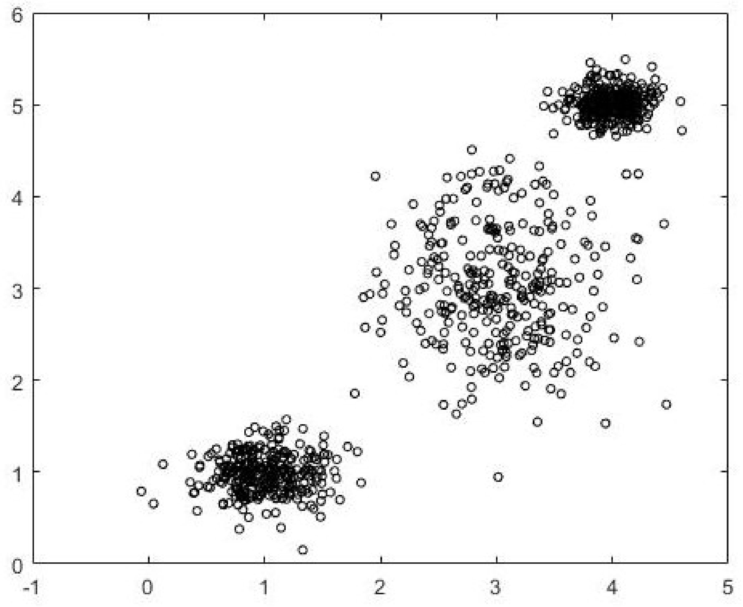
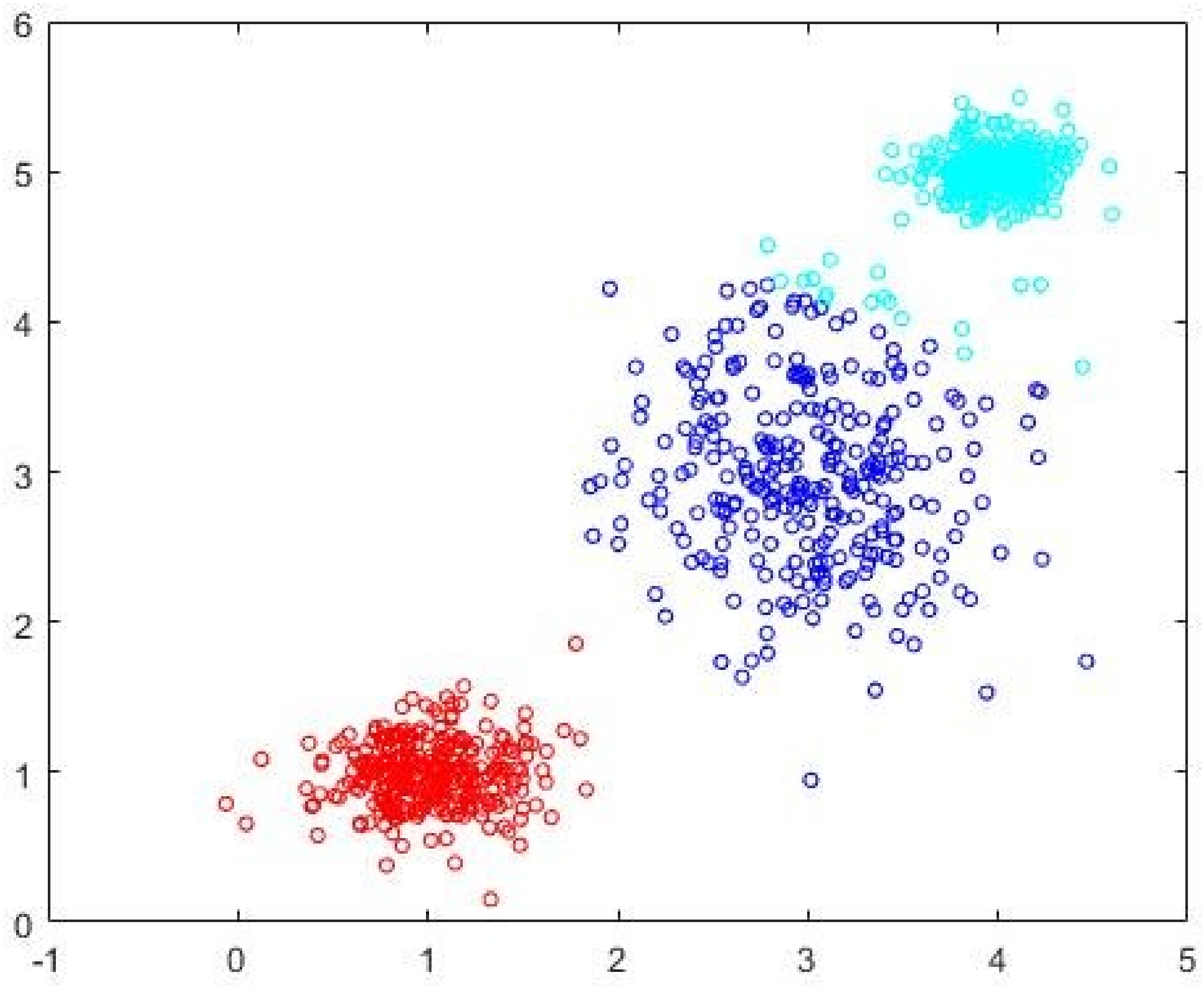
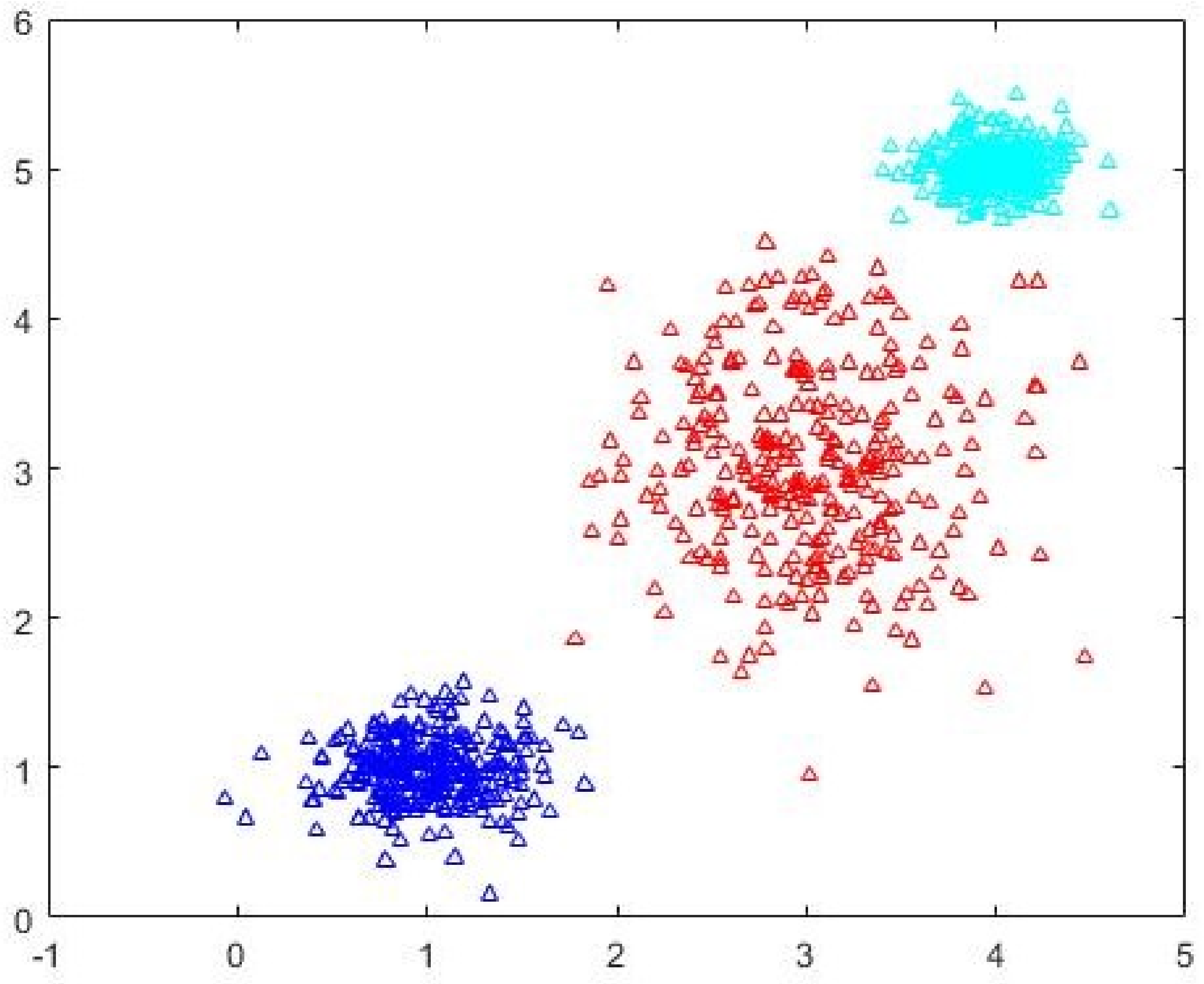
Data1 is a 900-point dataset in two dimensions. There are three well-separated and compact clusters with 300 data points in each cluster. The clusters are generated using normal distributions centered at (1,1), (3,3), and (4,5). The dataset is shown in Figure 2. The three-cluster FCM-AO partition is shown in Figure 3 and the three-cluster CDE-FCM after cluster prototype initialization is shown in Figure 4. The quality of the CDE-FCM can be seen to be marginally better than randomly initialized FCM-AO.

FCM-AO, PSO-V, GAKFCM, and EwFCM are run for c = 2 to c = 30. For ADEFC and CDE-FCM the vector representation is of length 60 with d = 2 and c_max = 30. The run-time parameters are chosen such as the convergence criteria for all algorithms are roughly the same. For comparison, the run-time of the different algorithms is presented in

Table 3. Runtime of algorithms for Data1.

	FCM-AO	ADEFC	PSO-V	GAKFCM	EwFCM	CDE-FCM
Run time (s)	2.85	8.39	5.67	8.45	4.11	8.45

. As can be seen, there is not much to be gained by using sophisticated schemes to address the problems of prototype initialization and unknown number of clusters for a small well-separated dataset as Data1. The naïve version of FCM-AO with random initializations works as well as any other scheme and in a fraction of the time.

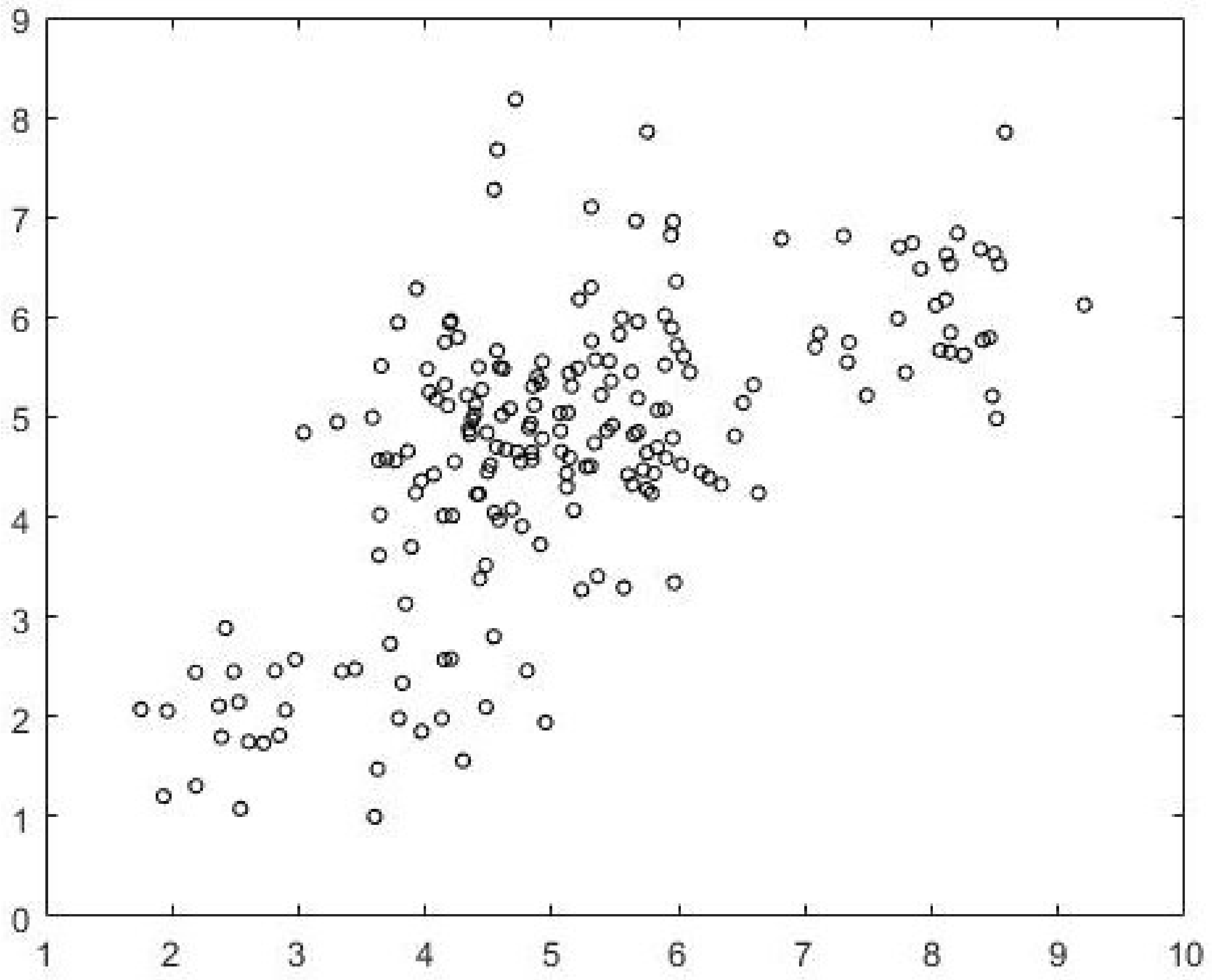
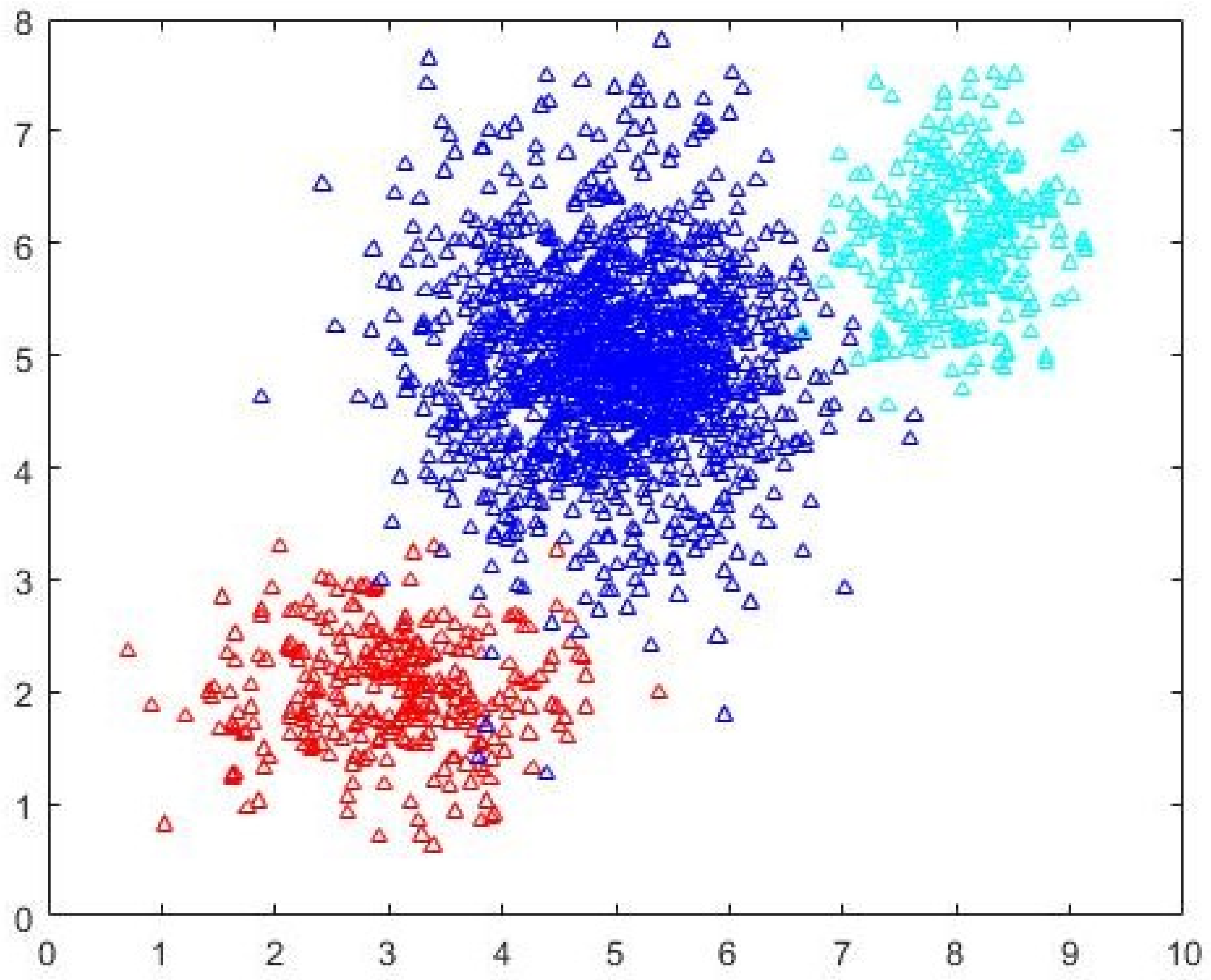
Data2 is a 2000-point dataset in two dimensions. Unlike Data1, the separation between the clusters is not well defined. The data is generated using three normal distributions centered at (3,2), (5.5,5.5) and (8.5,6). The intercluster variance is greater than that in Data1. The dataset is shown in Figure 5. FCM-AO, PSO-V, GAKFCM and EwFCM are run for c = 2 to c = 45. For ADEFC and CDE-FCM, the vector representation is of length 90 with d = 2 and c_max = 45. FCM-AO, GAKFCM, and EwFCM identify c = 5 as the most-optimal cluster. On the other hand, the evolutionary algorithm-based approaches, viz. PSO-V, ADEFC and the proposed CDE-FCM correctly identify the c = 3 partition. 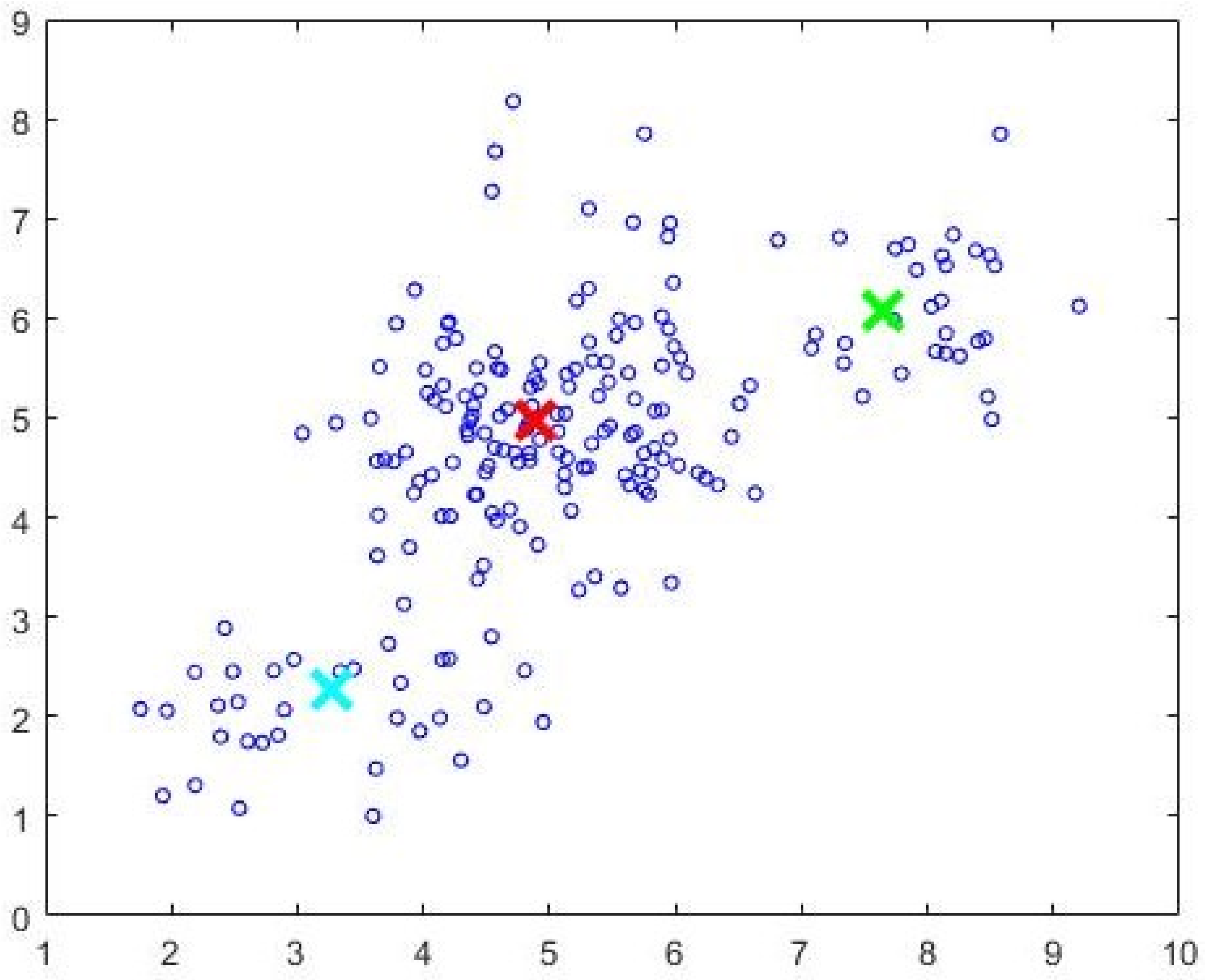In fact, the terminating elite population in CDE-FCM has 22% individuals that encode for c = 3 and 10% that encode for c = 5. The best subset of cardinality 200 as identified by Algorithm 2 is shown in Figure 6 and the initial cluster prototypes evolved by the CDE (Algorithm 3) are shown in Figure 7. 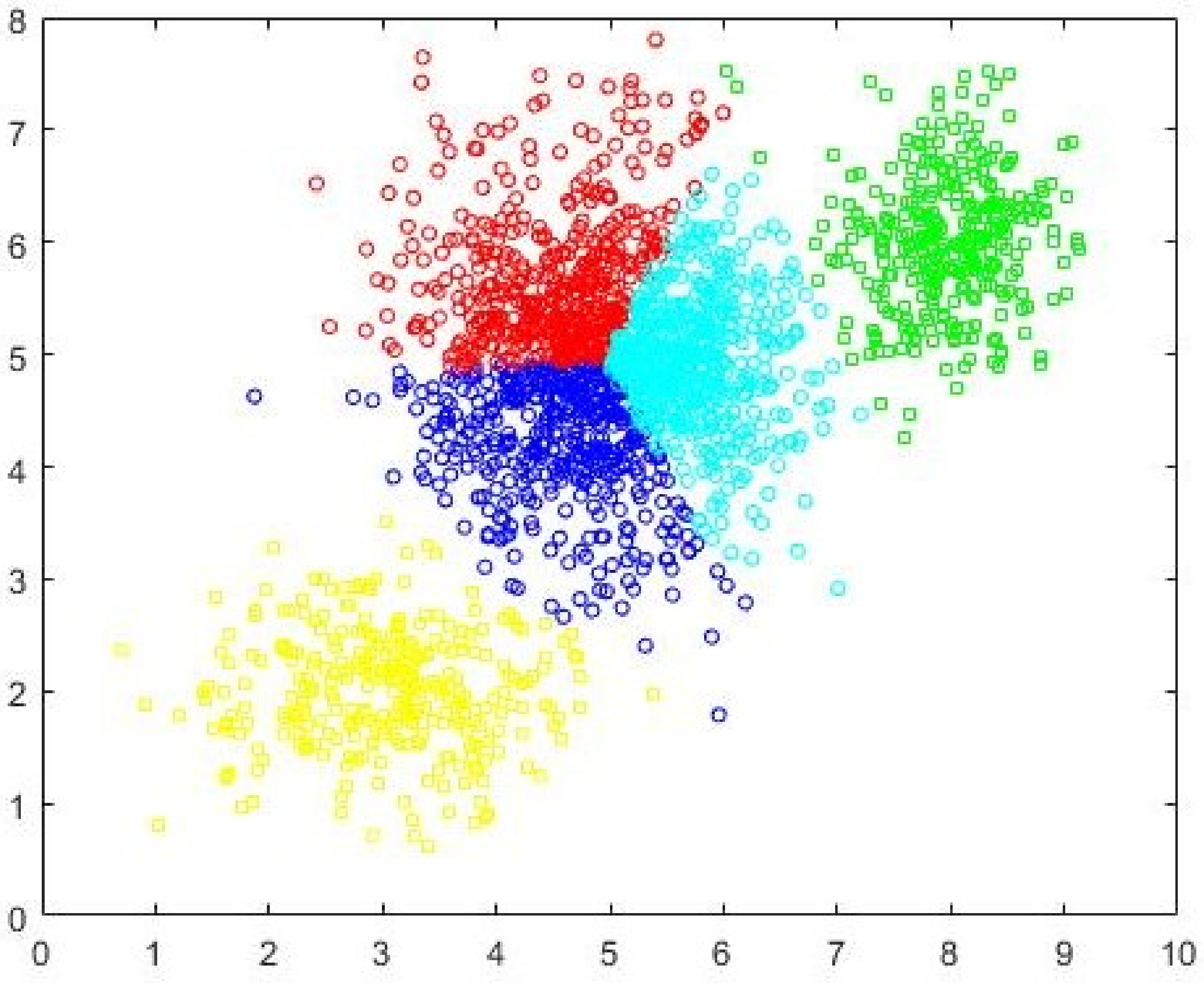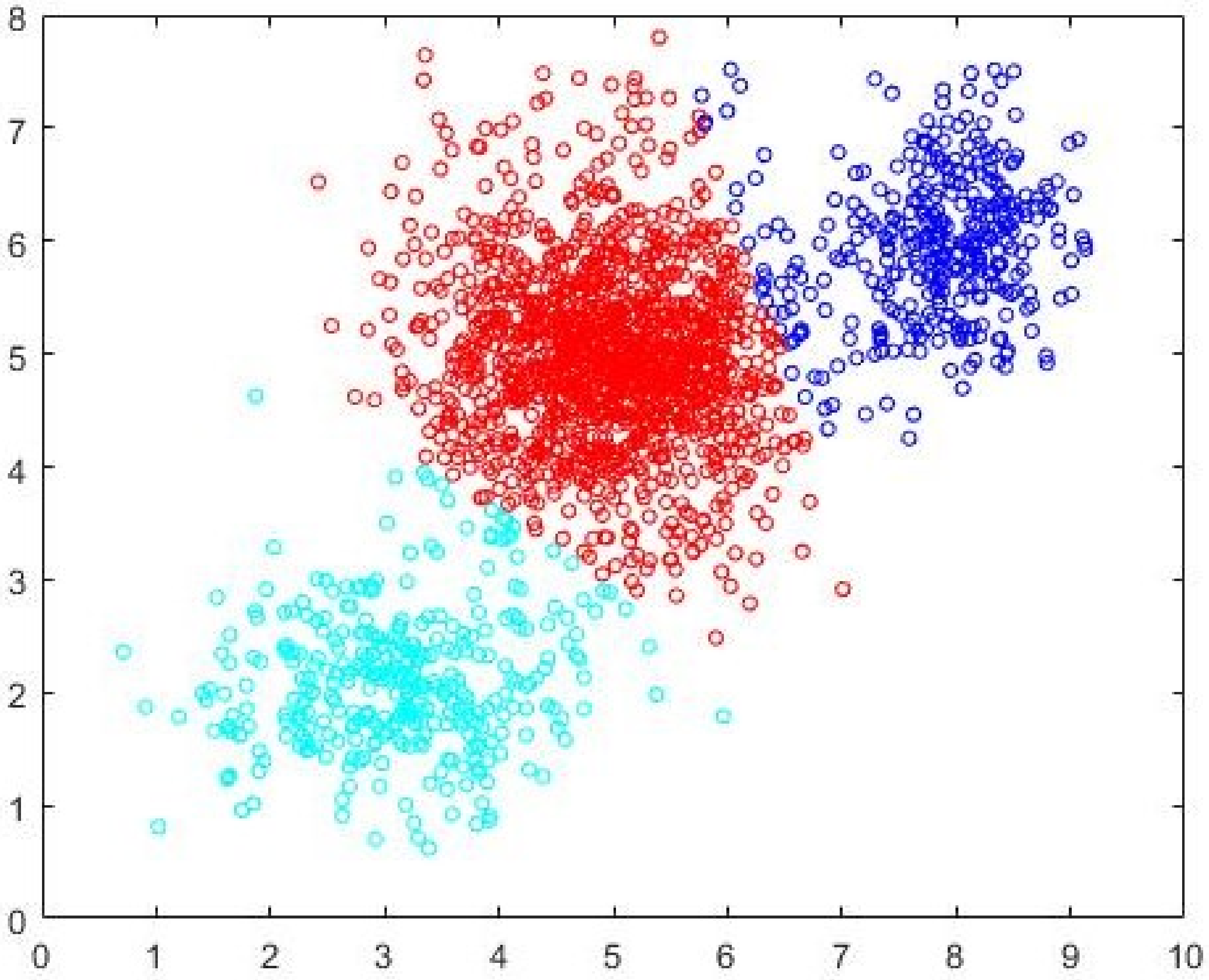The c = 5 partition as identified by FCM-AO as the most optimal partition is shown in Figure 8 and the c = 3 partition as identified by FCM-AO is shown in Figure 9. The correct c = 3 partition as identified by CDE-FCM with evolved initial prototypes is shown in Figure 10. By simple visual inspection, it can be said that the quality of the partition in Figure 10 is better than that in Figure 9 (same c = 3). The fact that FCM-AO with randomly initialized cluster prototypes identifies c = 5 as better than c = 3 on the basis of all cluster validity measures shows the promise of the proposed method. After the initial cluster prototypes are identified by Algorithm 3, the FCM-AO converged on an average in 4.5 iterations over 10 implementations. This is in comparison to the naïve FCM-AO with random initialization which took at least 25 iterations for an average of 28 iterations with the same convergence criterion of ε = 0.001.

Iris data consists of n = 150 datapoints divided into three types of Iris flowers-Setosa, Virginica, and Versicolor with 50 samples in each class. Each sample has four associated features: sepal length, petal length, sepal width, and petal width. FCM-AO, PSO-V, GAKFCM and EwFCM are run for c = 2 to c = 12. For ADEFC and CDE-FCM the vector representation is of length 48 with d = 4 and c_max = 12. The performances of different algorithms as measured by the cluster validity criteria are listed in

Table 4. Performance of algorithms on Iris data.

	c	VB	VT	VK2	VR
FCM-AO	2	0.2302	0.0682	8.9245	0.4789
	3	0.1349	0.1371	19.235	0.5529
	9	0.0284	0.3672	67.224	0.5849
ADEFC	9	0.0296	0.3619	71.344	0.5849
PSO-V	2	0.2311	0.0671	8.9382	0.4762
	3	0.1245	0.1371	19.235	0.5529
	9	0.0278	0.3774	67.334	0.5872
GAKFCM	2	0.2372	0.0680	8.9263	0.4821
	3	0.1262	0.1371	18.936	0.5587
EwFCM	3	0.1263	0.1362	19.292	0.5529
	4	0.1021	0.1942	32.039	0.6232
	9	0.0287	0.3672	71.348	0.5869
CDE-FCM	2	0.2235	0.0590	8.4385	0.4741

. Two classes (Versicolor and Virginica) are known to be linearly inseparable from each other although Setosa is linearly separable from the other classes [63] and therefore many algorithms identify the c = 2 solution as the most optimal one. Almost 20% of the candidate vectors in the terminating elite population of CDE-FCM encoded for c = 2 while 18% encoded for c = 3 with an equal number encoding for c = 9. The cluster prototypes identified by CDE-FCM in almost all candidates (>85%) in the terminating elite population are almost optimal, and a further application of FCM-AO converges on average in 4.1 iterations over 10 independent runs of the algorithm. On the other hand, the best-performing instance of the naïve FCM-AO with random initializations took 22 iterations.

Cancer data has 683 datapoints in two classes (malignant and benign). The data has 9 features (attributes)—clump thickness, cell size uniformity, cell shape uniformity, single epithelial cell size, bare nuclei, bland chromatin, normal nucleoli, and mitoses. There are 440 instances belonging to the benign cluster and 243 instances in the malignant cluster. The cancer dataset is known to be linearly inseparable and it is often difficult for clustering algorithms to achieve high levels of accuracy with this dataset. FCM-AO, PSO-V, GAKFCM and EwFCM are run for c = 2 to c = 26. For ADEFC and CDE-FCM the vector representation is of length 234 with d = 9 and c_max = 26. The performances of different algorithms as measured by the cluster validity criteria are listed in

Table 5. Performance of algorithms on cancer data.

	c	VB	VT	VK2	VR
FCM-AO	2	0.1233	0.0121	12.897	0.2868
	8	0.0129	0.6792	128.329	0.3862
ADEFC	2	0.1234	0.0123	12.775	0.2854
PSO-V	2	0.1293	0.0129	12.292	0.2841
	8	0.0137	0.6822	137.850	0.3922
GAKFCM	2	0.1224	0.0174	12.325	0.2833
	8	0.0193	0.6891	129.825	0.3851
EwFCM	2	0.1239	0.0132	12.457	0.2857
	8	0.0174	0.6891	135.839	0.3823
CDE-FCM	2	0.1197	0.0121	12.775	0.2803

. Little more than 18% of the candidate vectors in the terminating elite population of CDE-FCM encoded for c = 2 while approximately 15% of candidate vectors encoded for c = 8. The cluster prototypes identified by CDE-FCM in 72% of the candidates in the terminating elite population are almost optimal, and a further application of FCM-AO converges on average in 8.5 iterations over 10 independent runs of the algorithm. On the other hand, the best-performing instance of the naïve FCM-AO with random initializations took 31 iterations.

Glass data has 214 different glass samples with 9 features (refractive index, weight percent of corresponding oxide of Na, Mg, Al, Si, K, Ca, Ba, and Fe). There are 6 different types of glasses—building window (float), building window (non-float), vehicle window (float), container glass, tableware glass and headlamp glass. FCM-AO, PSO-V, GAKFCM and EwFCM are run for c = 2 to c = 15. For ADEFC and CDE-FCM the vector representation is of length 135 with d = 9 and c_max = 15. The performances of different algorithms as measured by cluster validity criteria are listed in

Table 6. Performance of algorithms on glass data.

	c	VB	VT	VK2	VR
FCM-AO	5	0.8251	0.1925	12.854	3.332
	6	0.8149	0.1786	12.779	3.297
ADEFC	5	0.8135	0.1883	12.775	3.472
PSO-V	5	0.8238	0.1937	12.854	3.974
	8	0.9244	0.2215	32.975	8.773
GAKFCM	5	0.8188	0.1875	12.695	3.224
	6	0.8275	0.1786	12.702	3.133
EwFCM	6	0.8175	0.1775	12.972	3.297
	8	0.8924	0.2232	37.395	9.725
CDE-FCM	6	0.8077	0.1760	12.715	3.109

. Almost all cluster validity indices agreed, and all algorithms produced very similar partitions at either c = 5, c = 6, and c = 8.

Wine dataset has 178 samples of wine differentiated by 13 attributes—percent contents of alcohol, malic acid, ash, magnesium, total phenols, flavonoids, nonflavonoid phenols, proanthocyanins, alkalinity of ash, color intensity, OD280/OD315 of diluted wines (protein content), and proline content. The wines are categorized into three classes (red, white, and rosé) with 59 instances in the first cluster, 71 in the second, and the rest in the third cluster. FCM-AO, PSO-V, GAKFCM, and EwFCM are run for c = 2 to c = 13. For ADEFC and CDE-FCM the vector representation is of length 169 with d = 13 and c_max = 13. The performances of different algorithms as measured by cluster validity criteria are listed in

Table 7. Performance of algorithms on Wine data.

	c	VB	VT	VK2	VR
FCM-AO	3	1.025	0.0997	8.726	2.970
ADEFC	4	1.133	0.1029	12.339	3.892
PSO-V	3	1.025	0.0987	8.697	2.835
GAKFCM	3	1.025	0.0997	8.645	2.754
EwFCM	3	1.175	0.0984	8.772	2.663
CDE-FCM	3	1.025	0.0984	8.597	2.754

. The clusters are well-defined, and all the cluster validity measures reach their minimum at either c = 3 or c = 4.

Wine Quality dataset has 1898 samples of wines divided into 11 classes (quality scores ranging from 0 to 10). The data are defined over 11 attributes—fixed acidity, volatile acidity, citric acid, residual sugar, chlorides, free SO₂, total SO₂, density, pH, sulphates, and alcohol content. This is the largest of the UCI datasets tested for this work both in terms of cardinality and dimensions. FCM-AO, PSO-V, GAKFCM and EwFCM are run for c = 2 to c = 45. For ADEFC and CDE-FCM the vector representation is of length 495 with d = 11 and c_max = 45. The performances of different algorithms as measured by cluster validity criteria are listed in

Table 8. Performance of algorithms on wine quality data.

	c	VB	VT	VK2	VR
FCM-AO	8	8.775	0.3721	72.456	5.978
	10	13.942	0.9885	125.814	8.775
	11	22.857	0.9925	216.380	12.394
	12	23.617	1.0225	229.773	12.945
ADEFC	10	14.332	0.9885	120.035	8.674
PSO-V	8	8.456	0.3389	70.990	5.825
	10	13.880	0.9727	118.336	8.650
	11	21.352	0.9880	207.350	12.218
	12	21.445	1.0225	219.872	12.945
GAKFCM	8	8.356	0.3392	71.855	5.978
	11	21.335	0.9891	208.392	12.218
EwFCM	8	8.470	0.3391	70.990	5.824
	10	13.442	0.9738	115.275	8.458
	11	21.832	0.9890	208.360	12.394
	12	21.975	1.0225	220.825	12.945
CDE-FCM	12	21.329	1.0225	217.375	12.885

. FCM-AO, PSO-V, GAKFCM, and EwFCM identify at least 8 of the classes with moderately high accuracy. Accuracy decreases for c = 11 as is evident from the cluster validity measures. ADEFC identifies c = 10 clusters, with an accuracy below 90% while the proposed CDE-FCM identifies 12 clusters with initial cluster centers almost optimal for 8 of the real classes. The FCM-AO implemented with cluster prototypes identified by CDE-FCM converges on an average of 12 iterations over 10 independent runs, while FCM-AO randomly initialized converges after an average of 33 iterations for c = 8 and 37 iterations for c = 11.

6. Case Study—Rolling Bearing Fault Analysis

Rolling element bearings are commonly used in supporting rotor components and assemblies in rotating machinery. Bearing defects can lead to undesirable vibrations, noise, or machine failure. Bearing fault diagnosis has been a subject of great importance in machine condition monitoring, predictive maintenance, and machine failure prevention and analysis [64]. Bearings conditions are presented in [65]. Techniques used in fault severity evaluation in rolling bearings are reviewed and discussed in [66]. The review is mainly focused on data-driven approaches such as signal processing for extracting the fault signatures associated with the fault degradation, and the approaches that are used to identify degradation patterns. Modern predictive maintenance techniques are increasingly adopting data analysis techniques such as pattern recognition and machine learning for bearing fault diagnosis. In this case study using the proposed cluster initialization method, wavelet analysis is used to process vibration signals from three bearing cases—no fault, inner race fault, and ball fault, under varying rotating speeds.

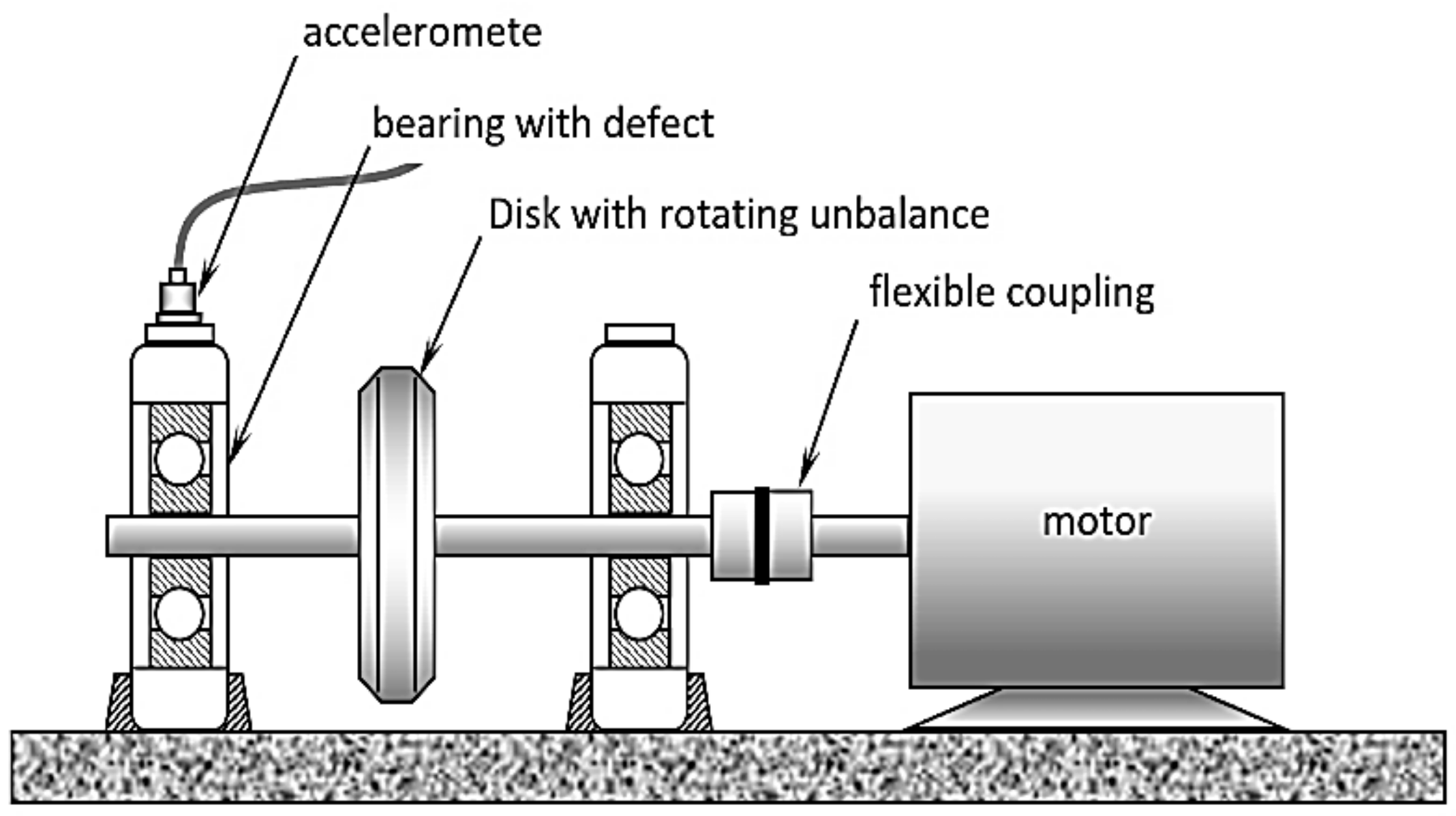
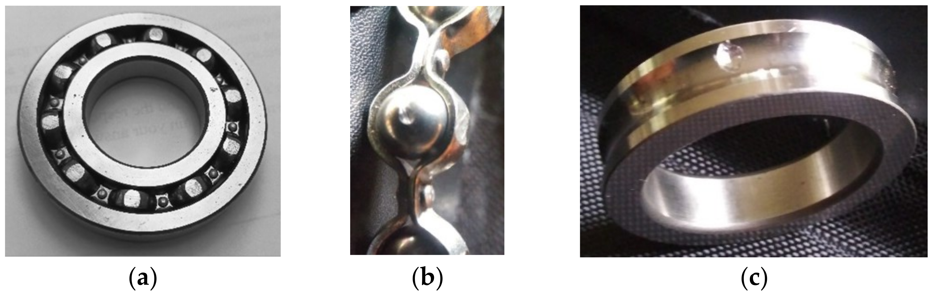
A schematic of the experimental setup is shown in Figure 11. The faults are introduced as a single rough surface spot simulating pitting wear and are created by using a small grinder as shown in Figure 12. The rotor is run at 10 different speeds (from 500 rpm to 1400 rpm) in increments of 100 rpm. At each speed level, vibration signals are acquired using a PCB accelerometer (model PCB 302A) which is mounted on the outboard test bearing as indicated in Figure 10. The sampling rate is 10,000 samples/s. A radial load of about 2000 lb was kept constant during all tests. A small unbalance mass is added to the rotor to introduce sustained periodic vibration excitation.

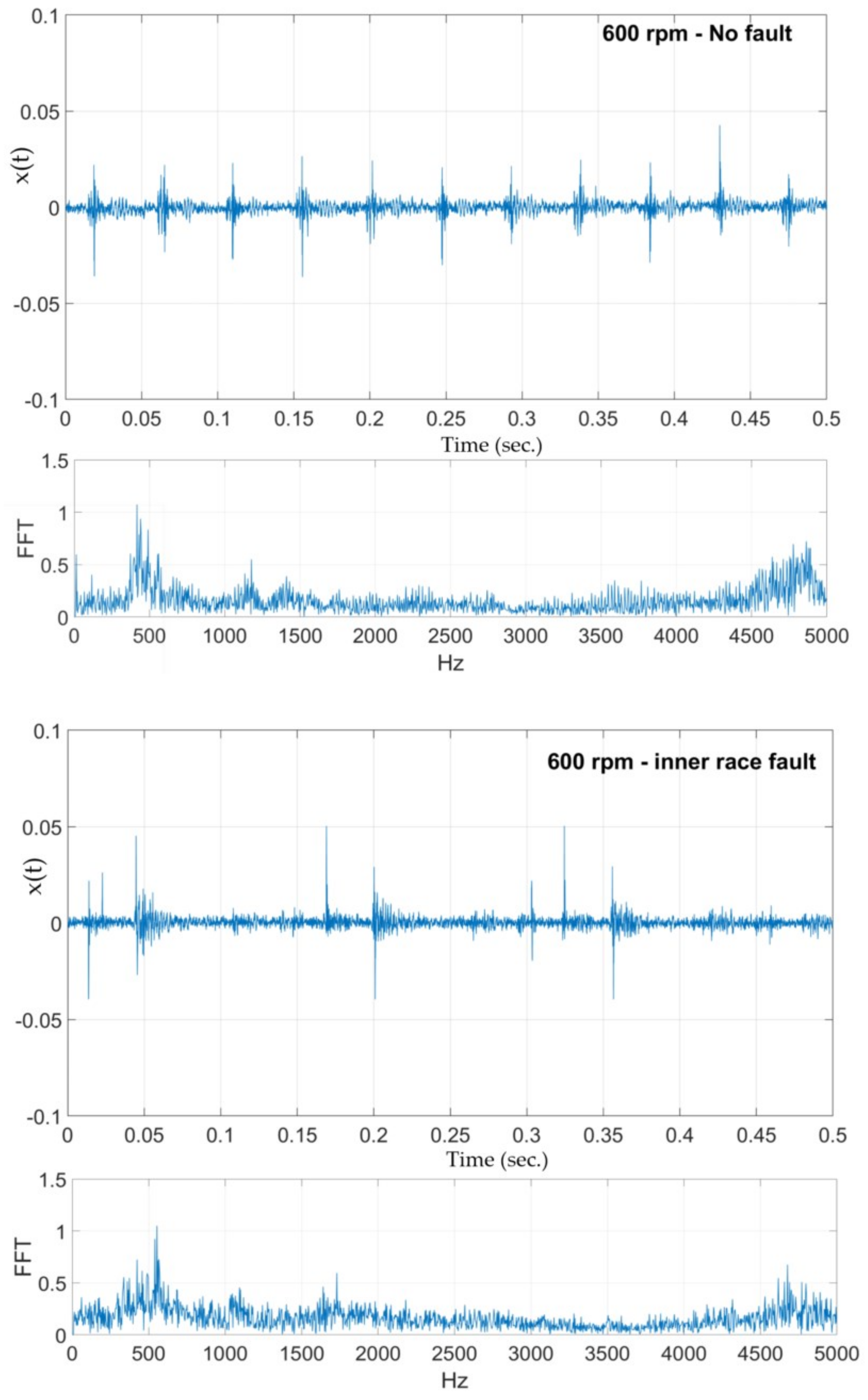
Three sets of samples are collected, each for 0.5 s. The analysis is performed for each of the three sets, followed by sets obtained using a 50% overlap between the non-overlapping sets resulting in five sample sets (3 non-overlapping sets and 2 overlapping sets) for a single operating condition—speed and type of fault (10 different speeds and 3 fault conditions including no fault). The raw time series is analyzed for statistical features such as mean, variance, standard deviation, skewness, and kurtosis. The times series are also subject to fast Fourier transform (FFT) and continuous wavelet transform (CWT) techniques. Figure 13 shows two sample raw vibration time series and their corresponding frequency spectrum obtained using FFT. After experimenting with several wavelet transform functions, the ‘Mexican hat’ and the Coiflet wavelet functions were used. The CWT implementation was performed using MATLAB’s wavelet toolbox. MATLAB’s CWT can be considered as a filter that scales a mother wavelet function along the time axis. At each scale, the CWT function will superimpose the scaled mother wavelet wave form over a segment of the signal under analysis. The similarities and differences between the form of the wavelet wave and the signal being analyzed are determined by CWT as,

$$C(a,T)={\displaystyle \int \frac{1}{\sqrt{a}}\psi (t)\left(\frac{t-T}{a}\right)x(t)dt}$$

(25)

where $\psi (t)$ represents the CWT mother wavelet function which is shifted in time by T and dilated or contracted by a factor and then correlated with the vibration signal represented by x(t).

All feature attributes are scaled and normalized across the column before clustering. The datasets are unlike others used in the paper—high dimensional data with relatively low cardinality. The idea is to see if the fault conditions can themselves be or if any combination of operating speed and fault condition can be partitioned. The datasets are described below:

BearingData1 is three non-overlapping segments with 16 FFT averages, n = 90, d = 16

BearingData2 is three non-overlapping segments with 64 Mexican Hat averaged wavelet coefficients, n = 90, d = 64

BearingData3 is three non-overlapping segments with 64 Coiflet-averaged wavelet coefficients, n = 90, d = 64

BearingData4 is three non-overlapping segments with kurtosis, skewness, RMS, and crest factors for 10 wavelet approximations and 10 wavelet details, n = 90, d = 80.

We also use a low dimensional data with non-overlapping and overlapping regions of the raw data (50% overlap). BearingData5 is three non-overlapping and two overlapping segments with four statistical features of the raw time signal—mean, skewness, standard deviation, and kurtosis, n = 150, d = 4.

The performance of the proposed method is compared with FCM-AO with random initialization of cluster prototypes using the four cluster validity indices. FCM-AO is implemented for c = 2 to c = 10. The vector representation used in CDE-FCM is d × 10. The results are tabulated in

Table 9. Performance of FCM-AO and CDE-FCM for five bearing fault datasets.

	c	VB	VT	VK2	VR
BearingData1, n = 90
FCM-AO	3	0.0245	1.2238	10.3762	1.8856
	5	0.0291	2.1925	22.4657	2.5320
	10	0.0132	2.5490	43.6115	6.9894
CDE-FCM	3	0.0239	1.2197	9.3250	1.7534
BearingData2, n = 90
FCM-AO	3	0.4578	17.895	71.965	5.3372
	5	0.5120	23.559	123.189	7.8900
	10	0.3251	14.358	53.172	4.3256
CDE-FCM	5	0.5052	19.856	112.885	7.2505
BearingData3, n = 90
FCM-AO	3	0.7925	8.6690	45.890	3.897
	5	0.8456	12.367	119.559	4.673
	10	1.6251	22.145	145.335	8.212
CDE-FCM	3	0.8280	8.5241	36.879	3.865
BearingData4, n = 90
FCM-AO	3	0.8955	8.356	67.189	2.9836
	6	0.7341	5.3536	50.338	2.5620
	10	1.3802	12.7467	121.298	3.2461
CDE-FCM	6	0.6821	5.1130	48.827	2.5465
BearingData5, n = 150
FCM-AO	3	0.0026	1.2876	8.9281	0.3653
	6	0.0012	1.1926	6.7172	0.3156
	10	0.0104	1.8927	11.602	0.7253
CDE-FCM	6	0.0011	1.2110	6.5670	0.3267

.

The proposed algorithm CDE-FCM almost always outperforms FCM-AO. In cases where the three natural groupings are not found, CDE-FCM finds approximately 6 clusters which are decoded as two subclusters based on speed (high and low) in most cases. The accuracy, precision, and recall rate of both FCM-AO and CDE-FCM are similar meaning they uncover very similar clusters although with FCM-AO it is often difficult to ascertain the optimal number of clusters.

A comparative evaluation is performed using sensitivity analysis. In clustering evaluation, a true positive (TP) is defined as the decision that assigns two similar data objects in the same cluster and a true negative (TN) is a decision that assigns two dissimilar objects to different clusters. These are both desirable outcomes. The errors can either be a false-positive (FP) decision for an assignment of two dissimilar objects to the same cluster or a false-negative (FN) decision when two similar objects are assigned to different clusters. These metrics are evaluated using pairwise measurements—for a dataset of cardinality n, there are n(n − 1)/2 pairs of objects. The precision (P) and recall (R) are defined as,

$$P=\frac{TP}{TP+FP},\hspace{0.17em}R=\frac{TP}{TP+FN}$$

(26)

The Rand index RI measures the percentage of decisions that are correct (also called the accuracy). The F-score is a measure of the harmonic mean of the method’s precision and recall. The F-score is implemented as F₁ in this paper (which gives equal weight to precision and recall) [67].

$$RI=\frac{TP+TN}{TP+FP+FN+TN},\hspace{0.17em}{F}_1=\frac{2PR}{P+R}$$

(27)

Results of the sensitivity analysis comparing CDE-FCM with FCM-AO are provided in

Table 10. Comparative evaluation of FCM-AO and CDE-FCM for five bearing fault datasets.

	TP	FP	TN	FN	P	R	RI	F1
BearingData1, n = 90, c = 3
FCM-AO	1295	721	1366	263	0.642	0.675	0.664	0.658
CDE-FCM	1481	694	1404	426	0.681	0.777	0.720	0.725
BearingData2, n = 90, c = 5
FCM-AO	1326	1926	1228	525	0.589	0.716	0.638	0.646
CDE-FCM	1497	612	1478	418	0.710	0.782	0.742	0.744
BearingData3, n = 90, c = 3
FCM-AO	1205	629	1516	655	0.657	0.648	0.679	0.652
CDE-FCM	1422	598	1498	487	0.704	0.745	0.729	0.724
BearingData4, n = 90, c = 6
FCM-AO	1375	826	1075	729	0.625	0.654	0.612	0.639
CDE-FCM	1457	683	1190	675	0.680	0.683	0.661	0.682
BearingData5, n = 150, c = 6
FCM-AO	4219	1622	4143	1191	0.772	0.780	0.748	0.750
CDE-FCM	4522	1433	4291	929	0.760	0.830	0.789	0.793

. As can be seen, the proposed method CDE-FCM achieves accuracies of approximately 75% with two of the five datasets. The best accuracy of FCM-AO approaches 75% for only one of the five datasets. The F₁ score equally weighing precision and recall for CDE-FCM is also better than FCM-AO for all five datasets. This is a promising result that shows the superiority of the proposed method over the original FCM with randomized initialization.

7. Conclusions and Directions of Future Work

A novel method of initializing cluster prototypes for fuzzy c-means (FCM) is presented in this paper. The method also simultaneously finds the optimal number of clusters in the partition. These two constitute the biggest drawbacks of clustering techniques such as FCM. Many attempts have been made in addressing the two issues-we present a very detailed review of the existing literature in this paper. The concept presented in this paper not only complements the body of work in this field but is also a non-trivial improvement on present techniques. We propose a co-evolutionary multi-population differential evolution-based technique to evolve a candidate vector that would encode for the most optimal set of initial cluster prototypes to use and also for the optimal number of clusters to find. This is based on a smaller subset of the original data thus reducing effort during evolution. The best subset is chosen based on a sparse sampling statistic from literature. A novel fitness evaluation function based on two cluster validity measures is also proposed. The proposed method called cooperative differential evolution for fuzzy c-means (CDE-FCM) is compared to some state-of-art improvements of FCM and also to the original FCM with random initial cluster prototypes implemented for a range of values for the number of clusters. The comparison is performed using a distinct set of cluster validity indices. In many of the cases with synthetic two-dimensional data and larger dimensional data from the UCI ML repository, the proposed algorithm performs better than the methods compared, and in almost all the cases, is almost as effective as the best of the other methods. The proposed method is also used on a real-world experimental dataset to partition rolling-bearing fault data. The technique worked well in real time and with very minimal improvements can be deployed to a live data analysis project such as this.

For future work, modifications to improve the proposed methodology will be investigated. Although the fitness evaluation and candidate evolution in the multi-population method are not resource intensive for parallel implementation, they can both be improved further. Statistical testing to evaluate the level of significance in performance improvement of the proposed method will also be performed as part of future work. This will result in ranking the comparative clustering methods used in this paper over other datasets from the UCI ML repository and on other benchmark datasets.

References

1. Everitt, B. Cluster Analysis; Wiley: Chichester, West Sussex, UK, 2011. [Google Scholar]
2. Bezdek, J.C. Pattern Recognition with Fuzzy Objective Function Algorithms; Plenum Press: New York, NY, USA, 1981. [Google Scholar]
3. Dunn, J.C. A fuzzy relative of the ISODATA process and its use in detecting compact well-separated clusters. J. Cybern. 1973, 3, 32–57. [Google Scholar] [CrossRef]
4. Bezdek, J.C.; Ehrlich, R.; Full, W. FCM: The fuzzy c-means clustering algorithm. Comput. Geosci. 1984, 10, 191–203. [Google Scholar] [CrossRef]
5. Bezdek, J.C.; Keller, J.; Krishnapuram, R.; Pal, N. Fuzzy Models and Algorithms for Pattern Recognition and Image Processing; Springer Science & Business Media LLC: Berlin/Heidelberg, Germany, 1999; Volume 4. [Google Scholar]
6. Pal, N.R.; Bezdek, J.C. On cluster validity for the fuzzy c-means model. IEEE Trans. Fuzzy Syst. 1995, 3, 370–379. [Google Scholar] [CrossRef]
7. Lee, M. Fuzzy cluster validity index based on object proximities defined over fuzzy partition matrices. In Proceedings of the 2008 IEEE International Conference on Fuzzy Systems (IEEE World Congress on Computational Intelligence), Hong Kong, China, 1–6 June 2008; pp. 336–340. [Google Scholar]
8. Zhang, X.-B.; Jiang, L. A new validity index of fuzzy c-means clustering. In Proceedings of the IEEE International Conference on Intelligent Human-Machine Systems and Cybernetics (IHMSC’09), Hangzhou, China, 26–27 August 2009; pp. 218–221. [Google Scholar]
9. Saha, I.; Maulik, U.; Bandyopadhyay, S. A new differential evolution based fuzzy clustering for automatic cluster evolution. In Proceedings of the IEEE International Advance Computing Conference (IACC’09), Patiala, India, 6–7 March 2009; pp. 706–711. [Google Scholar]
10. Yue, S.; Wang, J.-S.; Wu, T.; Wang, H. A new separation measure for improving the effectiveness of validity indices. Inf. Sci. 2010, 180, 748–764. [Google Scholar] [CrossRef]
11. Fukuyama, Y. A new method of choosing the number of clusters for the fuzzy c-mean method. In Proceedings of the 5th Fuzzy Systems Symposium 1989, Poznan, Poland, 28–30 September 1989; pp. 247–250. [Google Scholar]
12. Xie, X.L.; Beni, G. A validity measure for fuzzy clustering. IEEE Trans. Pattern Anal. Mach. Intell. 1991, 13, 841–847. [Google Scholar] [CrossRef]
13. Bensaid, A.M.; Hall, L.O.; Bezdek, J.C.; Clarke, L.P.; Silbiger, M.L.; Arrington, J.A.; Murtagh, R.F. Validity-guided (re)clustering with applications to image segmentation. IEEE Trans. Fuzzy Syst. 1996, 4, 112–123. [Google Scholar] [CrossRef] [Green Version]
14. Tang, Y.; Sun, F.; Sun, Z. Improved validation index for fuzzy clustering. In Proceedings of the American Control Conference, Portland, OR, USA, 8–10 June 2005; pp. 1120–1125. [Google Scholar]
15. Kwon, S.H. Cluster validity index for fuzzy clustering. Electron. Lett. 1998, 34, 2176–2177. [Google Scholar] [CrossRef]
16. Pakhira, M.K.; Bandyopadhyay, S.; Maulik, U. Validity index for crisp and fuzzy clusters. Pattern Recognit. 2004, 37, 487–501. [Google Scholar] [CrossRef]
17. Wu, K.-L.; Yang, M.-S. A cluster validity index for fuzzy clustering. Pattern Recognit. Lett. 2005, 26, 1275–1291. [Google Scholar] [CrossRef]
18. Wu, C.-H.; Ouyang, C.-S.; Chen, L.-W.; Lu, L.-W. A new fuzzy clustering validity index with a median factor for centroid-based clustering. IEEE Trans. Fuzzy Syst. 2015, 23, 701–718. [Google Scholar] [CrossRef]
19. Wang, J. A new clustering validity function for the fuzzy c-means algorithm. In Proceedings of the American Control Conference, Wuhan, China, 6–7 June 2009; pp. 2477–2480. [Google Scholar]
20. Rezaee, M.R.; Lelieveldt, B.B.F.; Reiber, J.H.C. A new cluster validity index for the fuzzy c-mean. Pattern Recognit. Lett. 1998, 19, 237–246. [Google Scholar] [CrossRef]
21. Zhu, L.F.; Wang, J.S.; Wang, H.Y. A novel clustering validity function of FCM clustering algorithm. IEEE Access 2019, 7, 152289–152315. [Google Scholar] [CrossRef]
22. Frigui, H.; Krishnapuram, R. A robust competitive clustering algorithm with applications in computer vision. IEEE Trans. Pattern Anal. Mach. Intell. 1999, 21, 450–465. [Google Scholar] [CrossRef] [Green Version]
23. Pelleg, D.; Moore, A.W. X-means: Extending K-means with efficient estimation of the number of clusters. In Proceedings of the 17th International Conference on Machine Learning (ICML’00), San Francisco, CA, USA, 29 June–2 July 2000; pp. 727–734. [Google Scholar]
24. Yang, M.-S.; Wu, K.-L. A similarity-based robust clustering method. IEEE Trans. Pattern Anal. Mach. Intell. 2004, 26, 434–448. [Google Scholar] [CrossRef] [PubMed]
25. Girolami, M. Mercer-kernel-based clustering in feature space. IEEE Trans. Neural Netw. 2002, 13, 780–784. [Google Scholar] [CrossRef] [Green Version]
26. Yujian, L. A clustering algorithm based on maximal θ-distant subtrees. Pattern Recognit. 2007, 40, 1425–1431. [Google Scholar] [CrossRef]
27. Liu, W.-Y.; Xiao, C.H.-J.; Wang, B.-W.; Shi, Y.; Fang, S.-F. Study on combining subtractive clustering with fuzzy c-means clustering. In Proceedings of the 2003 Winter Simulation Conference, Xi’an, China, 5 November 2003; pp. 2659–2662. [Google Scholar]
28. Chen, J.; Qin, Z.; Jia, J. A weighted mean subtractive clustering algorithm. Inf. Technol. J. 2008, 7, 356–360. [Google Scholar] [CrossRef] [Green Version]
29. Zou, K.-Q.; Wang, Z.-P.; Pei, S.-J.; Hu, M. A new initialization method for fuzzy c-means algorithm based on density. In Fuzzy Information and Engineering; Advances in Intelligent and Soft Computing; Springer Science & Business Media LLC: Berlin/Heidelberg, Germany, 2009; Volume 54, pp. 547–553. [Google Scholar]
30. Cardone, B.; Di Martino, F. A novel fuzzy entropy-based method to improve the performance of fuzzy c-means algorithm. Electronics 2020, 9, 554. [Google Scholar] [CrossRef] [Green Version]
31. Lei, T.; Jia, X.; Zhang, Y.; He, L.; Meng, H.; Nandi, A.K. Significantly fast and robust fuzzy c-means clustering algorithm based on morphological reconstruction and membership filtering. IEEE Trans. Fuzzy Syst. 2018, 26, 3027–3041. [Google Scholar] [CrossRef] [Green Version]
32. Ding, Y.; Fu, X. Kernel-based fuzzy c-means clustering algorithm based on genetic algorithm. Neurocomputing 2016, 188, 233–238. [Google Scholar] [CrossRef]
33. Li, D.; Han, Z.; Zhao, J. A novel level set method with improved fuzzy c-means based on genetic algorithm for image segmentation. In Proceedings of the 3rd International Conference on Big Data Computing and Communications (BIGCOM), Chengdu, China, 10–11 August 2017; pp. 151–157. [Google Scholar]
34. Franco, D.G.D.B.; Steiner, M.T.A. Clustering of solar energy facilities using a hybrid fuzzy c-means algorithm initialized by metaheuristics. J. Clean. Prod. 2018, 191, 445–457. [Google Scholar] [CrossRef]
35. Abdellahoum, H.; Mokhtari, N.; Brahimi, A.; Boukra, A. CSFCM: An improved fuzzy c-means image segmentation algorithm using a cooperative approach. Expert Syst. Appl. 2021, 166, 114063. [Google Scholar] [CrossRef]
36. Potts, J.C.; Giddens, T.D.; Yadav, S.B. The development and evaluation of an improved genetic algorithm based on migration and artificial selection. IEEE Trans. Syst. Man Cybern. 1994, 24, 73–86. [Google Scholar] [CrossRef]
37. Ding, W.; Feng, Z.; Andreu-Perez, J.; Pedrycz, W. Derived multi-population genetic algorithm for adaptive fuzzy c-means clustering. Neural Process. Lett. 2022, 1–25. [Google Scholar] [CrossRef]
38. Goh, C.K.; Tan, K.C.; Liu, D.S.; Chiam, S.C. A competitive and cooperative co-evolutionary approach to multi-objective particle swarm optimization algorithm design. Eur. J. Oper. Res. 2010, 202, 42–54. [Google Scholar] [CrossRef]
39. Antonio, L.M.; Coello Coello, C.A. Coevolutionary multiobjective evolutionary algorithms: Survey of the state-of-the-art. IEEE Trans. Evol. Comput. 2018, 22, 851–865. [Google Scholar] [CrossRef]
40. Ma, X.; Li, X.; Zhang, Q.; Tang, K.; Liang, Z.; Xie, W.; Zhu, Z. A survey on cooperative co-evolutionary algorithms. IEEE Trans. Evol. Comput. 2019, 23, 421–441. [Google Scholar] [CrossRef]
41. Hopkins, B. A new method of determining the type of distribution of plant individuals. Ann. Bot. 1954, 18, 213–226. [Google Scholar] [CrossRef]
42. Lawson, R.G.; Jurs, P.C. New index for clustering tendency and its application to chemical problems. J. Chem. Inf. Comput. Sci. 1990, 30, 36–41. [Google Scholar] [CrossRef]
43. Holgate, P. Tests of randomness based on distance measures. Biometrika 1965, 52, 345–353. [Google Scholar] [CrossRef]
44. Besag, J.E.; Gleaves, J.T. On the detection of spatial pattern in plant communities. Bull. Int. Stat. Inst. 1973, 45, 153–158. [Google Scholar]
45. Eberhardt, L.L. Some developments in distance sampling. Biometrics 1967, 23, 207–216. [Google Scholar] [CrossRef]
46. Cox, T.F.; Lewis, T. A conditioned distance ratio method for analyzing spatial patterns. Biometrika 1976, 63, 483–491. [Google Scholar] [CrossRef]
47. Banerjee, A.; Davé, R.N. Validating clusters using the Hopkins statistic. In Proceedings of the IEEE International Conference on Fuzzy Systems, Budapest, Hungary, 25–29 July 2004; pp. 149–153. [Google Scholar]
48. Adolfsson, A.; Ackerman, M.; Brownstein, N.C. To cluster, or not to cluster: An analysis of clusterability methods. Pattern Recognit. 2019, 88, 13–26. [Google Scholar] [CrossRef] [Green Version]
49. Storn, R.; Price, K. Differential evolution—A simple and efficient heuristic for global optimization over continuous spaces. J. Glob. Optim. 1997, 11, 341–359. [Google Scholar] [CrossRef]
50. Das, S.; Suganthan, P.N. Differential evolution: A survey of the state-of-the-art. IEEE Trans. Evol. Comput. 2011, 15, 4–31. [Google Scholar] [CrossRef]
51. Das, S.; Mullick, S.S.; Suganthan, P.N. Recent advances in differential evolution—An updated survey. Swarm Evol. Comput. 2016, 27, 1–30. [Google Scholar] [CrossRef]
52. Qin, A.K.; Huang, V.L.; Suganthan, P.N. Differential evolution algorithm with strategy adaptation for global numerical optimization. IEEE Trans. Evol. Comput. 2009, 13, 398–417. [Google Scholar] [CrossRef]
53. Mezura-Montes, E.; Velzquez-Reyes, J.; Coello-Coello, C.A. A comparative study of differential evolution variants for global optimization. In Proceedings of the Genetic and Evolutionary Computation Conference, Seattle, WA, USA, 8–12 July 2006; pp. 485–492. [Google Scholar]
54. Price, K.V. An introduction to differential evolution. In New Ideas in Optimization; Corne, D., Dorigo, M., Glover, V., Eds.; McGraw-Hill: London, UK, 1999; pp. 79–108. [Google Scholar]
55. Wang, Y.; Cai, Z.; Zhang, Q. Differential evolution with composite trial vector generation strategies and control parameters. IEEE Trans. Evol. Comput. 2011, 15, 55–66. [Google Scholar] [CrossRef]
56. Brest, J.; Zamuda, A.; Boskovic, B.; Maucec, M.S.; Zumer, V. Dynamic optimization using self-adaptive differential evolution. In Proceedings of the 2009 IEEE Congress on Evolutionary Computation, Trondheim, Norway, 18–21 May 2009; pp. 415–422. [Google Scholar]
57. Zhang, J.; Sanderson, A.C. JADE: Adaptive differential evolution with optional external archive. IEEE Trans. Evol. Comput. 2009, 13, 945–958. [Google Scholar] [CrossRef]
58. Maulik, U.; Bandyopadhyay, S. Performance evaluation of some clustering algorithms and validity indices. IEEE Trans. Pattern Anal. Mach. Intell. 2022, 24, 1650–1654. [Google Scholar] [CrossRef]
59. Kwon, S.H.; Kim, J.; Son, S.H. Improved cluster validity index for fuzzy clustering. Electron. Lett. 2021, 57, 792–794. [Google Scholar] [CrossRef]
60. Ren, M.; Liu, P.; Wang, Z.; Yi, J. A self-adaptive fuzzy c-means algorithm for determining the optimal number of clusters. Comput. Intell. Neurosci. 2016, 2016, 2647389. [Google Scholar] [CrossRef] [PubMed] [Green Version]
61. Runkler, A.; Katz, C. Fuzzy clustering by particle swarm optimization. In Proceedings of the IEEE International Conference on Fuzzy Systems, Vancouver, BC, Canada, 16–21 July 2006; pp. 601–608. [Google Scholar] [CrossRef]
62. UCI Machine Learning Repository. University of California, School of Information and Computer Science: Irvine, CA, USA. Available online: http://archive.ics.uci.edu/ml (accessed on 14 June 2022).
63. Tsai, D.-M.; Lin, C.-C. Fuzzy c-means based clustering for linearly and nonlinearly separable data. Pattern Recognit. 2011, 44, 1750–1760. [Google Scholar] [CrossRef]
64. Bently, D. Predictive maintenance through the monitoring and diagnostics of rolling element bearings. Bently Nev. Co. Appl. Note 1989, 44, 2–8. [Google Scholar]
65. El-Thalji, I.; Jantunen, E. A summary of fault modelling and predictive health monitoring of rolling element bearings. Mech. Syst. Signal Process. 2015, 60–61, 252–272. [Google Scholar] [CrossRef]
66. Cerrada, M.; Sánchez, R.-V.; Li, C.; Pacheco, F.; Cabrera, D.; Valente de Oliveira, J.; Vásquez, R.E. A review on data-driven fault severity assessment in rolling bearings. Mech. Syst. Signal Process. 2018, 99, 169–196. [Google Scholar] [CrossRef]
67. Schütze, H.; Manning, C.D.; Raghavan, P. Introduction to Information Retrieval; Cambridge University Press: Cambridge, UK, 2008; Volume 39. [Google Scholar]
Figure 1. Example of an initial cluster prototype candidate vector and associated masker.
Algorithms 15 00380 g001
Figure 2. Data1 (n = 900, c = 3, H = 0.9727).
Algorithms 15 00380 g002
Figure 3. FCM-AO with randomly initialized cluster prototypes for c = 3.
Algorithms 15 00380 g003
Figure 4. CDE-FCM with evolved initial cluster prototypes for c = 3.
Algorithms 15 00380 g004
Figure 5. Data2 (n = 2000, c = 3, H = 0.9184).
Algorithms 15 00380 g005
Figure 6. Best subset of Data2 using sparse sampling (n = 200, H = 0.9025).
Algorithms 15 00380 g006
Figure 7. Initial cluster prototype as calculated by CDE on best subset of Data2. The Xs mark the initial cluster prototype location.
Algorithms 15 00380 g007
Figure 8. Best partition by FCM-AO, c = 5 with randomly initialized cluster prototypes.
Algorithms 15 00380 g008
Figure 9. Partition by FCM-AO, c = 3 with randomly initialized cluster prototypes.
Algorithms 15 00380 g009
Figure 10. Partition by CDE-FCM, c = 3 with initial cluster prototypes shown in Figure 7.
Algorithms 15 00380 g010
Figure 11. Experimental setup.
Algorithms 15 00380 g011
Figure 12. (a) Ball bearing used in the test, (b) ball fault, (c) inner race fault.
Algorithms 15 00380 g012
Figure 13. Vibration time signatures and corresponding FFT spectrum for two cases.
Algorithms 15 00380 g013