Fair Benchmark for Unsupervised Node Representation Learning

Abstract

Most machine-learning algorithms assume that instances are independent of each other. This does not hold for networked data. Node representation learning (NRL) aims to learn low-dimensional vectors to represent nodes in a network, such that all actionable patterns in topological structures and side information can be preserved. The widespread availability of networked data, e.g., social media, biological networks, and traffic networks, along with plentiful applications, facilitate the development of NRL. However, it has become challenging for researchers and practitioners to track the state-of-the-art NRL algorithms, given that they were evaluated using different experimental settings and datasets. To this end, in this paper, we focus on unsupervised NRL and propose a fair and comprehensive evaluation framework to systematically evaluate state-of-the-art unsupervised NRL algorithms. We comprehensively evaluate each algorithm by applying it to three evaluation tasks, i.e., classification fine tuned via a validation set, link prediction fine-tuned in the first run, and classification fine tuned via link prediction. In each task and each dataset, all NRL algorithms were fine-tuned using a random search within a fixed amount of time. Based on the results for three tasks and eight datasets, we evaluate and rank thirteen unsupervised NRL algorithms.

1. Introduction

Networks are widely adopted to represent relations between objects in various disciplines. For instance, we leverage networks to study social ties [1], financial transactions [2], word co-occurrence [3], and protein–protein interactions [4]. When the network is small, traditional algorithms in graph theory can be used to analyze the network. Examples include clustering based on normalized cuts and node classification on the basis of label propagation. However, learning and prediction tasks in real-world networked systems have been incredibly complex, such as recommendations and advertising on large social networks with multifarious user-generated content [5], the completion of knowledge graphs with millions of entities [6], and fraud detection in financial transaction networks [7]. Hence, traditional graph theory cannot directly satisfy the demands of real-world network analysis tasks.

To fill this gap and utilize off-the-shelf machine-learning algorithms in large and sophisticated networks, node representation learning (NRL) [1,8] has been extensively investigated. Machine-learning algorithms often make default assumptions that instances are independent of each other, and their features exist in the Euclidean space. However, these are not applicable to networked data, because, usually, networks depict node-to-node dependencies and exist in non-Euclidean space. The goal of NRL is to learn a low-dimensional vector to represent each node, such that actionable patterns in the original networks and side information can be well-preserved in the learned vectors [9,10]. Furthermore, these low-dimensional representations can be directly leveraged by common machine-learning algorithms as feature vectors, or hidden layers can perform a wide variety of tasks, such as node classification [11,12], anomaly detection [13], community detection [14], and link prediction [15,16].

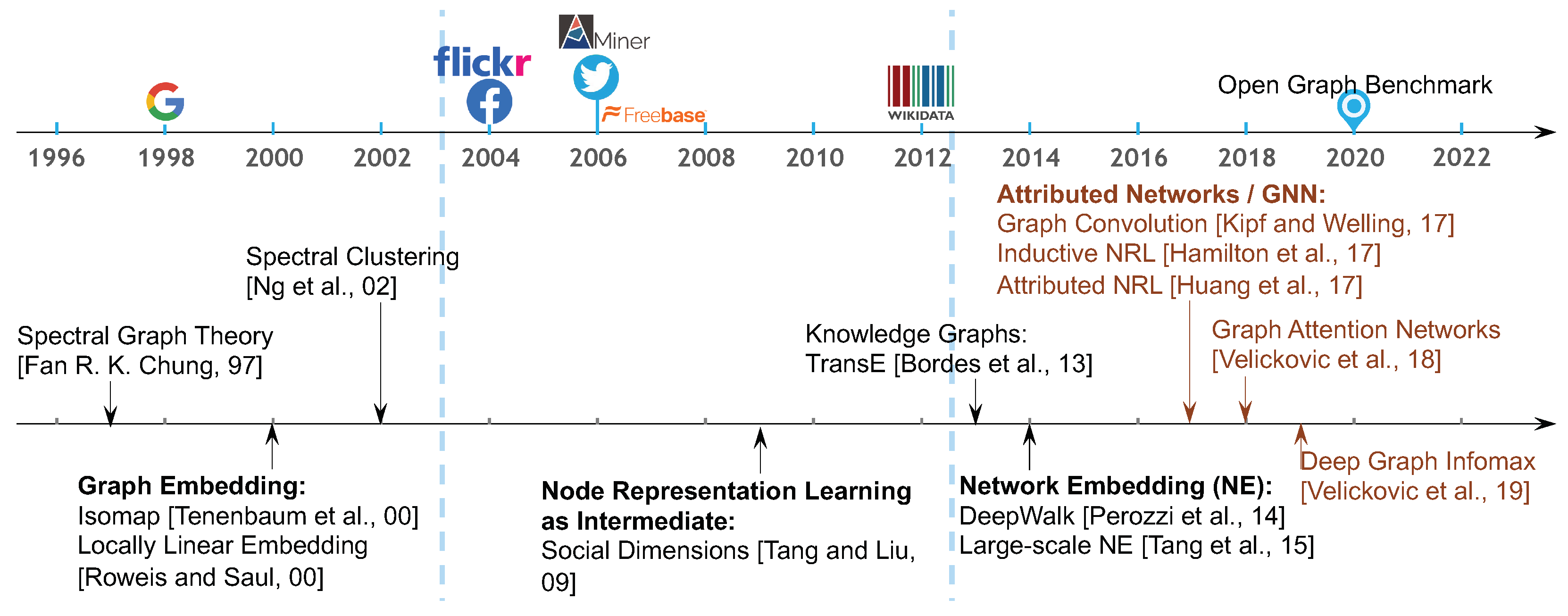
In the early 2000s, as illustrated in Figure 1, NRL was known as graph embedding [17,18,19], which was mainly used to perform dimensionality reduction for feature vectors. Its core idea can be summarized as two steps. First, given a set of instances, such as documents or images of faces, associated with feature vectors, we construct a new graph to connect all instances. Its ${(i,j)}^{\mathrm{th}}$ edge weight is set as the shortest path distance [18], reconstruction coefficient [20,21], or similarity [17] between nodes i and j in the feature vector space. Second, we apply multidimensional scaling [18] or eigen decomposition to the adjacency matrix or its variation [17,20]. In such a way, the learned node representations can be employed as the latent features of instances. It has been proven that most dimensionality reduction techniques, such as principal component analysis and linear discriminant analysis, could be reformulated as graph-embedding processes with constraints [19]. Meanwhile, efforts have also been devoted to utilizing NRL as an intermediate process to conduct clustering [22,23,24], known as spectral clustering. Its key idea is similar to graph embedding [19]. Based on feature vectors, we construct a new network depicting similarities between instances, and then calculate the eigenvectors of the graph Laplacian matrix of this new network. The learned eigenvectors serve as the latent representations of instances. To predict the clusters, a traditional clustering algorithm such as k-means is applied to the eigenvectors.

Later, since mid 2000s, with the rapid development of the web, especially social-networking sites, there has been an increase in the types and numbers of real-world networks available, such as Facebook, Flickr, and Twitter. NRL has been employed as an intermediate step when performing node classification [12,25,26] and visualizations [27] in real-world networks, including online social networks such as Flickr [26] and BlogCatalog [28], academic networks [25], molecule structures [27], and linked web pages [12]. With the boom in web-based networks and prediction tasks performed on them, node representation learning, also known as network embedding, was formally defined [1,10,29] in 2014 and has attracted intensive attention in recent years [30,31]. Since real-world networks are often large, alongside the major goal, i.e., preserving the topological structure information, scalability is another common objective of NRL algorithms [8,32]. The availability of networked data boosts the development of various NRL algorithms [33,34,35], because it is significant for different practical scenarios which need distinct and appropriate NRL solutions.

However, it has become challenging to track the state-of-the-art node representation learning algorithms, given that numerous methods are available in the literature. When an NRL algorithm is proposed, only a few baseline methods and datasets are included in the empirical evaluation. Moreover, different NRL studies may use different experimental settings, such as evaluation tasks, hardware environments, and ways of hyperparameter tuning. Therefore, the lack of fair and comprehensive evaluation of state-of-the-art NRL algorithms is preventing researchers and practitioners from tracking the effective NRL algorithms for specific scenarios.

In this paper, we focus on unsupervised node representation learning. There are three major challenges in developing a fair and comprehensive evaluation framework for unsupervised NRL. First, it is difficult to guarantee fair comparisons. The running times of different NRL algorithms vary significantly. These algorithms also have different numbers of hyper-parameters and search spaces. A fair evaluation framework should take the running time and hyperparameter tuning into consideration. Second, tailored evaluation tasks are needed to comprehensively assess each NRL algorithm. Node classification and link prediction are two widely adopted downstream tasks when evaluating NRL algorithms. However, for each task, there are many ways to tune hyperparameters. Third, as different NRL algorithms are originally implemented in distinct systems, it is not easy to integrate them into a unified environment for a fair comparison.

To bridge this gap, in this paper, we develop a fair and comprehensive evaluation framework for unsupervised node representation learning (FURL). Through the development of FURL, we aim to answer two research questions. (1) How can we fairly evaluate state-of-the-art unsupervised NRL algorithms, given that they have different efficiencies and distinct search spaces for hyperparameters? (2) On the basis of a fair evaluation protocol, how can we comprehensively evaluate each unsupervised NRL algorithm? Our contributions can be summarized as follows.

• We develop a novel evaluation framework—FURL, which could fairly and comprehensively evaluate unsupervised NRL algorithms.
• We enable fair comparisons by performing a random search and allowing a fixed amount of time to fine-tune each algorithm.
• We enable comprehensiveness by using three tailored evaluation tasks, i.e., classification fine tuned via a validation set, link prediction fine-tuned in the first run, and classification fine tuned via link prediction.
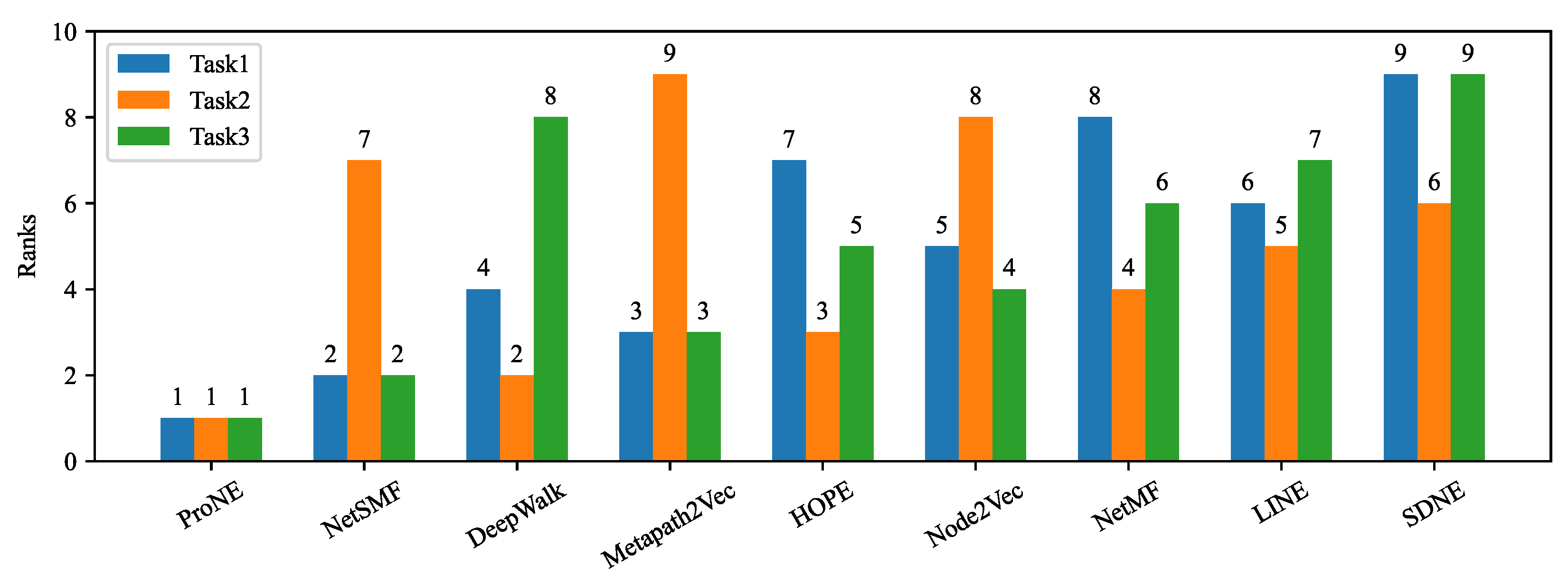
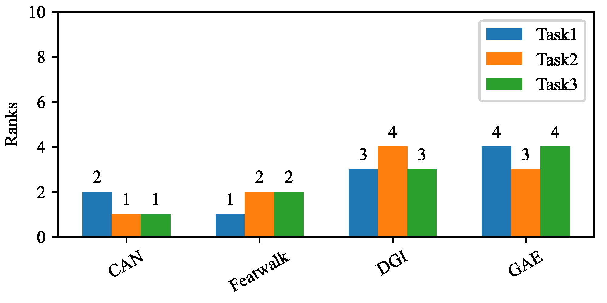
• We perform empirical studies by utilizing eight datasets and thirteen state-of-the-art unsupervised NRL algorithms. It is straightforward to extend these to more unsupervised NRL algorithms and datasets. Based on the systematic results from three tasks and eight datasets, we assess the overall rank of all thirteen algorithms.

2. Fair and Comprehensive Evaluation Algorithm—FURL

To help researchers and practitioners track the state-of-the-art unsupervised node representation learning methods, an ideal solution would have two properties. First, fairness. Existing methods are implemented using different experimental settings, including cross-validation settings, hyperparameter tuning methods, and total running time. It is important to design a mechanism to fairly compare these methods under the same setting. Second, comprehensiveness. The learned embedding representations are designed for different downstream tasks in general. It is desirable to evaluate all NRL algorithms comprehensively from multiple aspects. Additionally, when integrating these multiple evaluation results into an overall rank, the integration schema should be in line with human prior experience. For example, it is expected that an NRL algorithm with ranks $\{2,3,4\}$ (evaluated from three aspects) should rank higher than an NRL algorithm with ranks $\{3,3,3\}$. This is because the former NRL algorithm ranks second in the first aspects, indicating a significant potential.

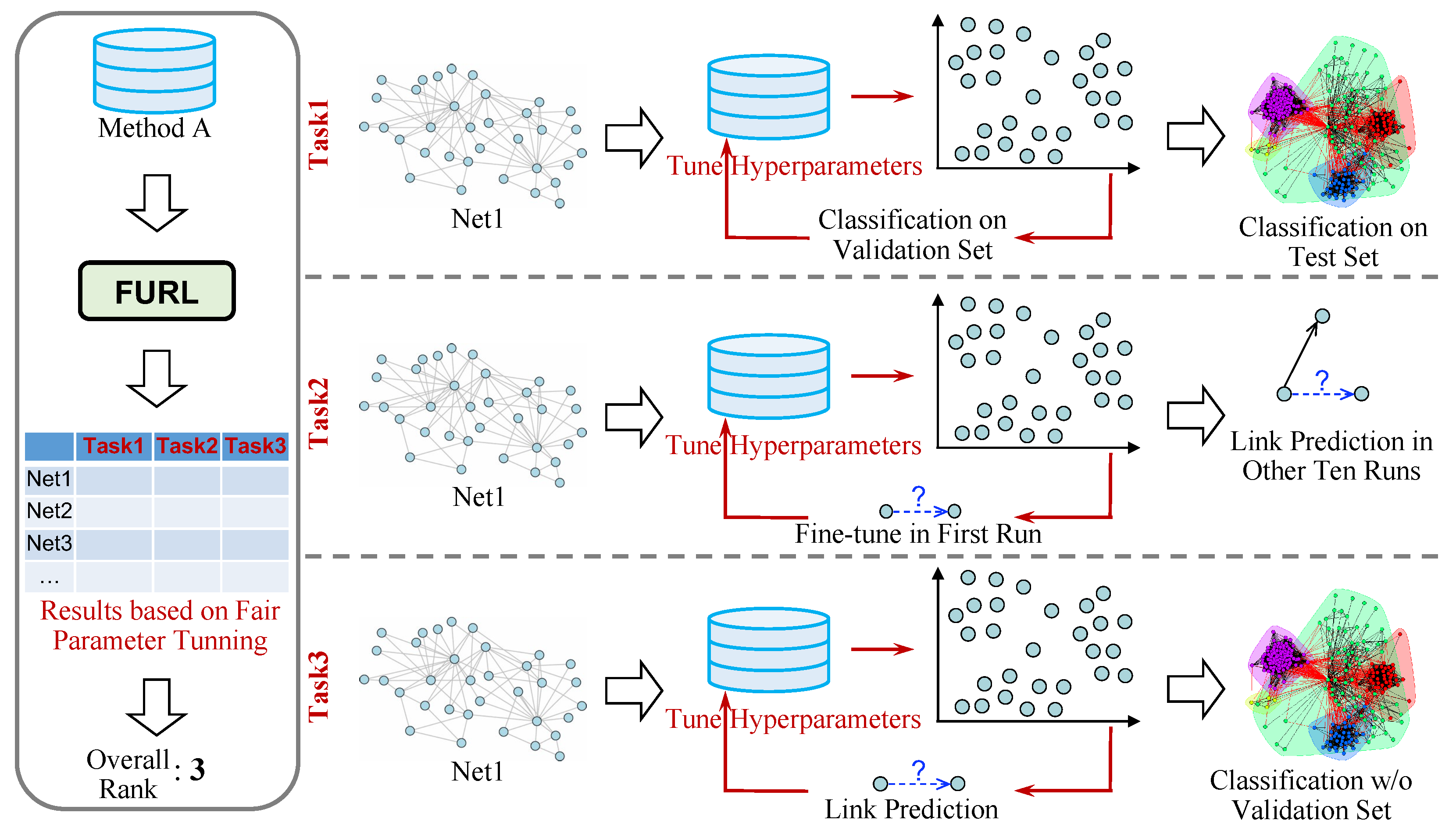
We propose a fair and comprehensive evaluation framework—FURL. Its core idea is illustrated in Figure 2. To systematically evaluate an NRL method, we apply it to performing three tasks. To make the comparisons fair, on each task, the total amount of hyperparameter tuning time and running time is the same for all methods. We now introduce the three tasks in detail. We design a tailored integration schema to combine evaluation results in three tasks. It would assess a comprehensive rank for each given NRL algorithm. We now introduce the three tasks in detail.

2.1. Task 1—Classification Fine Tuned via a Validation Set

Node classification has been widely used to evaluate embedding models [36,37]. As illustrated in Figure 2, Task 1 consists of three steps. First, given an NRL method, e.g., Method A, we apply it to embed the entire network, e.g., Net1, and learn embedding representations for all nodes. We use k-fold cross-validation to separate all the nodes into a training set and a test set. Second, we tune the hyperparameters of Method A in the first round (k rounds in total, corresponding to k folds), and then fix the hyperparameters for all k rounds. Specifically, in the first round, we employ $1/10$ of the training set as a validation set to tune hyperparameters. We leverage the embedding representations of the remaining training nodes ($9/10$) and their labels to train support vector machines (SVMs). Then, we use the trained SVMs to predict the classes of nodes in the validation set. Based on the classification performance on the validation set, we select the best hyperparameters for the embedding model, i.e., Method A. Third, after we have selected the best hyperparameters, we add the validation set back into the training set. Given the embedding representations learned by fine tuning model (with the best hyperparameters), we conduct k-fold cross-validation ten times, named as ten runs. In each run, there are k rounds. In each round, we use the labels of the training nodes to train SVMs, and use them to predict the classes of test nodes. The average of all $10k$ results on the test sets is employed as the final performance of Method A in Task 1.

In summary, we employ a simple process, i.e., using a validation set in the first round, to fine tune the embedding model. This is because efficiency is important for hyperparameter searching. After we have identified the best hyperparameters, we evaluate Method A by performing k-fold cross-validation ten times. This is because comprehensiveness is essential to the final evaluation result. It should be noted that the validation set is generated from the training set in the first round, so test data is not leaked in the hyperparameter tuning. Task 1 is not end-to-end.

2.2. Task 2—Link Prediction Fine Tuned in the First Run

Link prediction has also been widely used to evaluate embedding models. In this task, we evaluate the effectiveness of each NRL algorithm in preserving network patterns by applying the learned representations to recover unseen links. As illustrated in Figure 2, Task 2 consists of three steps. First, given a network, e.g., Net1, we randomly select $B/2$ node pairs that are connected as positive samples, and $B/2$ node pairs that are not connected as negative samples, where B denotes the total number of node pairs to be predicted. We remove the $B/2$ edges of the $B/2$ positive samples from the original network. Then, we apply the given NRL model, e.g., Method A, to embed the new network. We will employ the learned node representations to perform link prediction. Second, in the first run, we tune the hyperparameters of Method A. In particular, we mix the $B/2$ positive samples and $B/2$ negative samples and obtain a set with B node pairs. For each pair in the B node pairs, we denote its two nodes as i and j. We compute the inner product of the embedding representations of nodes i and j, and employ the inner product to indicate the probability of having a link between nodes i and j. After obtaining the inner products of all B pairs, we rank them and compute the average precision (AP) and area under the receiver operating characteristic curve (ROC AUC), indicating the performance of link prediction. Based on this link-prediction performance, we select the best hyperparameters for the embedding model, i.e., Method A. Third, we employ the selected best hyperparameters to conduct another ten runs. In each run, we randomly select $B/2$ positive samples and $B/2$ negative samples from the original network. We remove the $B/2$ edges of positive samples from the original network, and obtain a new network. We apply Method A with the selected best hyperparameters to embed the new network. We calculate the inner products of all B pairs, and we compute the AP and ROC AUC. The average of the results of the ten runs is employed as the final performance of Method A in Task 2.

In summary, we fine tune Method A in the first run and obtain the best hyperparameters. We employ the selected hyperparameters to perform another ten runs. In each run, a different set of B samples are utilized to conduct the evaluation, that is, a different network (after removing $B/2$ edges) is used to conduct embedding. Both the hyperparameter tuning and final evaluation are conducted in an unsupervised manner.

2.3. Task 3—Classification Fine Tuned via Link Prediction

One of the core purposes of learning embedding representations is to have low-dimensional representations ready, such that we can directly apply them to downstream tasks if needed. To simulate such a scenario, we propose Task 3, in which we fine tune the NRL model in an unsupervised manner, and then apply the learned unsupervised embedding representations to perform classification. In this task, the hyperparameter-tuning process is the same as the one in Task 2. The final evaluation process is also the same as the one in Task 1. As illustrated in Figure 2, Task 3 consists of four steps. First, given a network, we randomly select $B/2$ node pairs that are connected as positive samples, and $B/2$ node pairs that are not connected as negative samples. We remove the $B/2$ edges of the $B/2$ positive samples from the original network. We apply the given NRL model, e.g., Method A, to embed the new network. Second, we tune the hyperparameters of Method A based on link prediction. For each node pair in the B node pairs ($B/2$ negative samples and $B/2$ positive samples), we denote its two nodes as i and j. We compute the inner product of the embedding representations of nodes i and j, and employ the inner product to indicate the probability of having a link between nodes i and j. After obtaining the inner products of all the B pairs, we compute the AP and ROC AUC. Based on this link-prediction performance, we select the best hyperparameters for the embedding model, i.e., Method A. We apply the fine-tuned model (with the best hyperparameters) to the original network, and learn embedding representations. Third, we use k-fold cross-validation to separate all nodes into a training set and a test set. We use the representations of training nodes to train SVMs, and use them to predict the classes of test nodes. Fourth, we repeat step three ten times, i.e., conducting k-fold cross-validation ten times. The average of all $10k$ results of the test sets is employed as the final performance of Method A in Task 3.

2.4. Integration Schema for Overall Rank

FURL enables comprehensive evaluations of unsupervised NRL methods. It involves not only two prediction tasks, but also different ways of hyperparameter tuning. Although unsupervised NRL methods are generally trained without labels, the hyperparameter searching can be conducted with or without labeled data. In Task 1, we use labels to tune hyperparameters. In Tasks 2 and 3, we tune hyperparameters without using labels.

We apply each unsupervised NRL algorithm to perform the aforementioned three tasks on all datasets. In each task and each dataset, all algorithms are assigned a fixed amount of time to conduct hyperparameter tuning. They all use random search to tune hyperparameters. Thus, we can perform the evaluation in a fair way.

Let D denote the total number of datasets used in the evaluation. Let C denote the total number of unsupervised NRL algorithms that we have included in the experiments. Let $R_{ij}$ denote the rank of an algorithm, e.g., Method A, among all C algorithms, based on their performance in the $i^{\mathrm{th}}$ task on the $j^{\mathrm{th}}$ dataset. We collect the ranks of Method A as a matrix $\mathbf{R}\in {\mathbb{R}}^{3\times D}$. Then, the overall rank of Method A can be calculated by computing the rank product over all datasets and three tasks as follows. The rank product is a widely used approach to combine ranked lists. 

$$\begin{array}{c}\hfill S_{\mathrm{overallrank}}=f_{\mathrm{rank}}\left(\sqrt[3]{\prod _{i=1}^3{f}_{\mathrm{rank}}\left(\sqrt[D]{\prod _{j=1}^D{R}_{ij}}\right)}\right),\end{array}$$

(1)

 which can be simplified as follows,

$$\begin{array}{c}\hfill S_{\mathrm{overallrank}}=f_{\mathrm{rank}}(\sum _{i=1}^{3}log\left(f_{\mathrm{rank}}(\sum _{j=1}^{D}log{R}_{ij})\right)),\end{array}$$

(2)

where $f_{\mathrm{rank}}\left(\right)$ takes the result of Method A as input, compares it with the corresponding results of all other $C-1$ algorithms, and returns the rank of Method A as output. Equation (1) is simplified into Equation (2) by applying a logarithmic function to the output of rank products before computing ranks using $f_{\mathrm{rank}}\left(\right)$. Since the logarithmic operation is monotonic, this transformation does not affect the final ranks. As illustrated in Equation (2), our schema integrates the rank matrix $\mathbf{R}$ in two steps. First, we sum up the logarithm of the ranks of Method A on all D datasets. Then, $f_{\mathrm{rank}}\left(\right)$ can help us find the rank of Method A on the ith task. Second, we sum up the logarithm of the ranks of Method A on all three tasks. Finally, $f_{\mathrm{rank}}\left(\right)$ can return the overall rank of Method A.

In each step, we follow a map-and-aggregate policy. The ranks are first mapped using a logarithmic function, then aggregated by summing up. The mapping function needs to be monotone, aiming to maintain the order of algorithms after mapping. The simplified rank product indicates that an algorithm that ranks 2th, 3th, and 4th in the three tasks has a higher potential than an algorithm that ranks 3th, 3th, and 3th.

3. Unsupervised Node Representation Learning Algorithms and Datasets

We included nine unsupervised NRL algorithms that are designed for pure networks, and four unsupervised NRL algorithms that are designed for attributed networks.

3.1. Unsupervised Node Representation Learning Methods Used in FURL

For a fair comparison, we separate the existing unsupervised NRL methods into two categories based on whether associated attribute information is exploited for learning node representations. We carefully select nine methods dedicated to pure networks, and four methods for attributed network embedding. We present a detailed introduction of each method as follows. We also list the hyperparameters and their corresponding search space for each method in

Table 1. Hyperparameter search space of unsupervised NRL algorithms.

Algorithms	Hyperparameters & Search Space	Type
DeepWalk	number_walks: [5, 80]	int
	walk_length: [5, 80]	int
	window_size: [2, 40]	int
metapath2vec	window_size: [1, 20]	int
	min_count: [1, 10]	int
	walk_length: [5, 80]	int
	walk_num: [5, 80]	int
node2vec	p: {0.25, 0.5, 1, 2, 4}	discrete
	q: {0.25, 0.5, 1, 2, 4}	discrete
	walks: [5, 120]	int
	length: [5, 120]	int
	window: [5, 15]	int
NetMF	window: [5, 15]	int
ProNE	step: [5, 20]	int
	theta: [0, 1]	float
	mu: [0, 1]	float
NetSMF	window: [5, 15]	int
HOPE	lr: {0.1, 0.05, 0.01, 0.005, 0.001, 0.0005, 0.0001, 0.00005}	discrete
SDNE	nu1: {0.1, 0.05, 0.01, 0.005, 0.001, 0.0005, 0.0001, 0.00005}	discrete
	nu2: {0.1, 0.05, 0.01, 0.005, 0.001, 0.0005, 0.0001, 0.00005}	discrete
	alpha: {0.5, 0.4, 0.3, 0.2, 0.1, 0.05, 0.01, 0.005, 0.001, 0.0005, 0.0001, 0.00005}	discrete
	beta: {0, 0.1, 0.5, 5, 10, 15, 20, 30}	discrete
LINE	walk_length: [1, 100]	int
	walk_num: [1, 100]	int
	alpha: {0.5, 0.4, 0.3, 0.2, 0.1, 0.05, 0.01, 0.005, 0.001, 0.0005, 0.0001, 0.00005}	discrete
GAE	lr: {0.1, 0.05, 0.01, 0.005, 0.001, 0.0005, 0.0001, 0.00005}	discrete
	nb_epochs: [100, 1500]	int
	dropout: {0, 0.05, 0.1, 0.2, 0.3, 0.4, 0.5, 0.6, 0.7, 0.8, 0.9}	discrete
	hid_dim: {64, 128, 256}	discrete
	weight_decay: {0, $5\times {10}^{-4}$, ${10}^{-3}$}	discrete
CAN	lr: {0.1, 0.05, 0.01, 0.005, 0.001, 0.0005, 0.0001, 0.00005}	discrete
	nb_epochs: [100, 1500]	int
	dropout: {0, 0.05, 0.1, 0.2, 0.3, 0.4, 0.5, 0.6, 0.7, 0.8, 0.9}	discrete
DGI	lr: {0.1, 0.05, 0.01, 0.005, 0.001, 0.0005, 0.0001, 0.00005}	discrete
	nb_epochs: [100, 1500]	int
FeatWalk	alpha: [0, 1]	float
	num_paths: [10, 50]	int
	path_length: [5, 50]	int
	win_size: [5, 15]	int

.

3.1.1. Node Representation Learning for Pure Networks

We roughly categorize the existing NRL algorithms for pure networks into three classes, i.e., negative-sampling-based, matrix-factorization-based, and spectral-embedding-based. First, typical negative-sampling-based NRL algorithms includes DeepWalk [1], node2vec [31], and LINE [10]. Second, the typical matrix-factorization-based NRL algorithms include NetMF [38] and ProNE [39]. The key idea is to construct a proximity matrix and use singular value decomposition or other matrix-factorization algorithms to obtain the graph embedding. Third, the key idea of spectral embedding [22] is to compute the eigendecomposition of a normalized Laplacian matrix of the network. Spectral embedding based on NRL algorithms is not scalable, since the time complexity of eigendecomposition is $\mathbb{O}\left(N^2\right)$, where N denotes the total number of nodes.

• DeepWalk [1]: It first performs random walks on the network to convert it into a series of truncated node sequences. Then, it considers the recorded node sequences as a “corpus”, i.e., each node as a word and each sequence as a sentence, and applies a wording embedding technique to embed this “corpus”. In this way, we could learn a low-dimensional representation for each word (node), by using efficient wording embedding techniques.
• metapath2vec [40]: It formalizes meta-path-based random walks to construct the heterogeneous neighborhood of a node and then leverages a heterogeneous skip-gram model to learn node embedding representations.
• node2vec [31]: It performs balanced random walks to smoothly interpolate between breadth first sampling and depth first sampling.
• NetMF [38]: It proves that the existing negative sampling based on NRL algorithms could be considered as the variations of matrix factorization. Based on this theoretical analysis, it proposes an advanced matrix factorization for graphs.
• ProNE [39]: It first leverages sparse matrix factorization to learn the initial node representations. Then, it uses the high-order Cheeger’s inequality to modulate the spectral space of the graph and plot the initial representations on the adjusted graph. In this way, it can integrate the local smoothing information and the global clustering information.
• NetSMF [41]: It makes NetMF scalable by applying sparsification.
• HOPE [42]: It proposes to preserve asymmetric transitivity by approximating high-order proximity.
• SDNE [43]: It is a semi-supervised deep model with multiple layers of non-linear functions, aiming to preserve both the global and local network structures.
• LINE [10]: It can scale up to networks with millions of vertices and billions of edges. It has carefully designed objective functions that preserve both the first-order and second-order proximities, which are complementary to each other. An efficient and effective edge-sampling method is proposed for model inference, which solved the limitation of stochastic gradient descent on weighted edges without compromising efficiency.

3.1.2. Node Representation Learning for Attributed Networks

Definition 1

(Attributed Network). We refer the textual, image, numerical, or categorial data associated with each node as node attributes. A network with node attributes is defined as an attributed network. Examples include social networks with user-generated content, paper citation networks with abstracts, and protein–protein interaction networks with property descriptions.

In this paper, we select four typical unsupervised NRL algorithms for attributed networks, as follows.

• GAE [44]: It learns node embedding representations by reconstructing the network structure using autoencoders. A two-layer graph convolutional network is employed to conduct encoding.
• CAN [45]: It learns an embedding representation for each node and for each node attribute category. These two types of representations, i.e., node representations and attribute-category representations, are learned by variational autoencoders, and are in the same space.
• DGI [36]: It learns node embeddings by maximizing the mutual information between the local patch representation and the global graph representation.
• FeatWalk [46]: It advances random walks by introducing an attribute-enhanced walking strategy. In addition to random walks on the original network, it also allows walking from one node to another node through their shared node attribute categories. The joint truncated node sequences thus become more diverse.

To handle networks with node attributes, the field of graph neural networks (GNNs) has expanded rapidly in recent years [47,48,49,50]. Existing GNN models belong to the family of message passing frameworks [51,52], which update information for each node by recursively aggregating messages from its immediate neighbors in the graph. GNNs are generally classified into two categories, as follows.

The first class is spectral-based approaches [53,54,55,56,57,58,59], which generalize convolution operators on the grid-like data to graphs based on spectral graph theory [60]. GCN [56] employs the first-order Chebyshev polynomial approximation for graph convolution. In a follow-up, Xu et al. [59] analyze the expression power of GNNs according to the Weisfeiler–Lehman test for graph isomorphism. SGC [61] further simplifies GCN by removing the inner transformation matrices and non-linear activation functions. Although effective, they could struggle with modeling long-range dependencies because of a recursive message-passing restriction. APPNP [58] suggests replacing the original graph convolution matrix with a graph diffusion [62]. MixHop [63], N-GCN, [64] and Truncated Krylov [65] attempt to exploit multi-scale information in each layer [66]. The second line of research is spatial-based approaches [9,34,67,68], which stem from the vector domain and focus on using the graph structure directly for message propagation. One characteristic of these is to adopt the learnable aggregation function to aggregate neighbors. GraphSage [9] introduces mean/max/LSTM pooled aggregation functions to integrate neighborhood information. GAT [69] learns to assign different attention weights at each layer based on node features. Attention-based GNN models have achieved state-of-the-art results on several graph learning tasks [68,70,71].

However, most GNN models are dedicated to end-to-end classification. There is an issue when converting GNN models into unsupervised NRL methods. For example, if we directly employ one of the hidden layers as the learned embedding representations, GNN models would perform badly in Tasks 1, 2, and 3.

3.2. Real-World Datasets Used in FURL

We included eight publicly available real-world attributed networks in the experiments. Their statistical information is summarized in

Table 2. Statistics of all real-world datasets used in the experiments.

	# Nodes	# Edges	Dimension of Node Attributes	# Labels
Cora	2708	5278	1433	7
Flickr	7564	246,929	12,047	9
BlogCatalog	5196	171,743	8189	6
Citeseer	3327	4676	3703	6
Pubmed	19,717	44,327	500	3
Chameleon	2277	31,421	2325	5
Film	7600	26,752	932	5
Squirrel	5201	198,493	2089	5

. We will include more datasets in the future.

Cora, Citeseer, and Pubmed [72]. These are citation networks. Nodes correspond to papers and edges correspond to citations. Each node has a bag-of-words feature vector according to the paper abstract. Labels are defined as the academic topics.

Flickr [73]. It is a social-network dataset collected from Flickr. Node attributes denote the tags that reflect the users’ interests. Labels represent the groups that users have joined.

BlogCatalog [73]. It is a social network collected from a blog community. Nodes are web users and edges indicate the user interactions. Node attributes are generated from keywords of their blogs. Each user can register his/her blogs into six different predefined classes, which are considered as class labels for node classification.

Chameleon and Squirrel [74]. They are page–page networks collected from Wikipedia (December 2018), based on a given topic (either chameleons or squirrels). Nodes represent articles from the English Wikipedia. Edges reflect mutual links between articles. Node features indicate the presence of particular nouns in the articles and the average monthly traffic from October 2017 to November 2018.

Film [58]. This dataset is the actor-only induced subgraph of the film–director–actor–writer network [75]. Each node corresponds to an actor, and the edge between two nodes denotes co-occurrence on the same Wikipedia page. Node features correspond to some keywords in the Wikipedia pages. The nodes are classified into five categories in terms of the words of an actor’s Wikipedia.

4. Results

We now introduce the evaluation results returned by our proposed algorithm—FURL.

4.1. Experimental Settings and Environment Configuration

To make it fair, for each dataset, the total given hyperparameter tuning time is fixed. When there are N nodes and X edges in a network, the total given time would be $max\{\alpha N,\beta X\}$ seconds, where $\alpha$ and $\beta$ are coefficients related to the hardware configuration and software environment. We set $\alpha =1.5$ and $\beta =0.1$ for balancing the efficiency and reliability of results. By default, we employ a random search to tune hyperparameters. In Task 1 and Task 3, we use a radial basis function (RBF) kernel SVM as the classifier. The performance of classification is evaluated by macro-averaged F1 and micro-averaged F1. In Task 2, the performance is measured by two standard metrics, i.e., area under the ROC curve (AUC) and average precision (AP) scores. In Tasks 2 and 3, we set B as $25\%$ of the total number of edges. This means that, in each run of Task 2, we randomly remove $12.5\%$ of edges. We integrate all of the thirteen unsupervised NRL algorithms into a unified software package. We perform all experiments in the same environment, i.e., a server with Intel Xeon Silver 4214R CPU @2.4GHz processors. The GPUs are GeForce RTX 3090 with 24 GB memory.

4.2. Overall Rank of Node Representation Learning Methods for Pure Networks

The overall ranks of unsupervised NRL methods for pure networks are summarized in Figure 3, which are computed based on Equation (2). Node attributes are not used in this evaluation. Their results in Tasks 1, 2, and 3, are summarized in

Table 3. Results in Task 1, i.e., classification fine tuned via validation set, on pure networks, using random search to tune hyperparameters. Best results are shown in bold.

		Cora	Flickr	BlogCatalog	Citeseer	Pubmed	Chameleon	Film	Squirrel
Macro-averaged F1	DeepWalk	$0.8066\pm 0.0205$	$0.6269\pm 0.0102$	$\mathbf{0.7661}\pm 0.0089$	$0.6187\pm 0.0160$	$0.8022\pm 0.0054$	$0.6932\pm 0.0249$	$0.1612\pm 0.0070$	$0.5527\pm 0.0152$
	metapath2vec	$0.8462\pm 0.0177$	$0.6164\pm 0.0115$	$0.7198\pm 0.0096$	$0.6558\pm 0.0170$	$\mathbf{0.8282}\pm 0.0062$	$0.6378\pm 0.0220$	$0.1769\pm 0.0065$	$\mathbf{0.5944}\pm 0.0144$
	node2vec	$0.8473\pm 0.0178$	$0.5922\pm 0.0109$	$0.7201\pm 0.0115$	$0.6551\pm 0.0168$	$0.8264\pm 0.0061$	$0.6659\pm 0.0217$	$0.1708\pm 0.0060$	$0.5435\pm 0.0163$
	NetMF	$0.8363\pm 0.0166$	$0.5941\pm 0.0098$	$0.6909\pm 0.0131$	$0.5693\pm 0.0147$	$0.8246\pm 0.0056$	$0.6544\pm 0.0188$	$0.1767\pm 0.0092$	$0.5163\pm 0.0139$
	ProNE	$0.8387\pm 0.0172$	$0.6405\pm 0.0095$	$0.7156\pm 0.0103$	$0.6664\pm 0.0144$	$0.8185\pm 0.0061$	$0.6914\pm 0.0199$	$\mathbf{0.1769}\pm 0.0070$	$0.5616\pm 0.0144$
	NetSMF	$0.8260\pm 0.0184$	$0.6661\pm 0.0098$	$0.7136\pm 0.0111$	$0.6037\pm 0.0154$	$0.8239\pm 0.0053$	$\mathbf{0.7004}\pm 0.0202$	$0.1703\pm 0.0066$	$0.5813\pm 0.0139$
	HOPE	$0.7929\pm 0.0191$	$\mathbf{0.7045}\pm 0.0097$	$0.7488\pm 0.0110$	$0.5221\pm 0.0168$	$0.7827\pm 0.0065$	$0.6485\pm 0.0226$	$0.1708\pm 0.0065$	$0.5387\pm 0.0153$
	SDNE	$0.3479\pm 0.0214$	$0.3738\pm 0.0112$	$0.5506\pm 0.0143$	$0.2362\pm 0.0087$	$0.4442\pm 0.0058$	$0.5994\pm 0.0230$	$0.0851\pm 0.0028$	$0.3661\pm 0.0191$
	LINE	$\mathbf{0.8510}\pm 0.0168$	$0.6142\pm 0.0090$	$0.7476\pm 0.0119$	$\mathbf{0.6697}\pm 0.0152$	$0.8246\pm 0.0056$	$0.5962\pm 0.0218$	$0.1709\pm 0.0064$	$0.5279\pm 0.0136$
Micro-averaged F1	DeepWalk	$0.8201\pm 0.0172$	$0.6315\pm 0.0107$	$\mathbf{0.7696}\pm 0.0090$	$0.6673\pm 0.0146$	$0.8156\pm 0.0053$	$0.6902\pm 0.0249$	$0.2493\pm 0.0091$	$0.5521\pm 0.0156$
	metapath2vec	$0.8554\pm 0.0154$	$0.6226\pm 0.0109$	$0.7249\pm 0.0098$	$0.6999\pm 0.0155$	$\mathbf{0.8384}\pm 0.0057$	$0.6372\pm 0.0223$	$0.2440\pm 0.0078$	$\mathbf{0.5959}\pm 0.0146$
	node2vec	$\mathbf{0.8604}\pm 0.0146$	$0.5957\pm 0.0116$	$0.7254\pm 0.0114$	$0.6950\pm 0.0155$	$0.8366\pm 0.0058$	$0.6642\pm 0.0223$	$0.2471\pm 0.0078$	$0.5486\pm 0.0164$
	NetMF	$0.8459\pm 0.0146$	$0.5977\pm 0.0101$	$0.6998\pm 0.0125$	$0.6084\pm 0.0150$	$0.8354\pm 0.0052$	$0.6530\pm 0.0196$	$0.2460\pm 0.0107$	$0.5210\pm 0.0140$
	ProNE	$0.8503\pm 0.0150$	$0.6450\pm 0.0093$	$0.7234\pm 0.0099$	$0.7083\pm 0.0137$	$0.8294\pm 0.0055$	$0.6893\pm 0.0202$	$0.2443\pm 0.0094$	$0.5630\pm 0.0143$
	NetSMF	$0.8361\pm 0.0167$	$0.6689\pm 0.0099$	$0.7230\pm 0.0103$	$0.6450\pm 0.0140$	$0.8337\pm 0.0050$	$\mathbf{0.6978}\pm 0.0211$	$0.2437\pm 0.0099$	$0.5828\pm 0.0137$
	HOPE	$0.8049\pm 0.0164$	$\mathbf{0.7071}\pm 0.0101$	$0.7566\pm 0.0105$	$0.5803\pm 0.0154$	$0.7963\pm 0.0059$	$0.6493\pm 0.0215$	$0.2438\pm 0.0094$	$0.5402\pm 0.0155$
	SDNE	$0.4586\pm 0.0219$	$0.3852\pm 0.0113$	$0.5638\pm 0.0144$	$0.3535\pm 0.0169$	$0.5827\pm 0.0078$	$0.5960\pm 0.0225$	$\mathbf{0.2594}\pm 0.0105$	$0.3776\pm 0.0185$
	LINE	$0.8601\pm 0.0137$	$0.6217\pm 0.0091$	$0.7550\pm 0.0121$	$\mathbf{0.7113}\pm 0.0137$	$0.8351\pm 0.0053$	$0.5971\pm 0.0224$	$0.2474\pm 0.0086$	$0.5317\pm 0.0133$

,

Table 4. Results in Task 2, i.e., link prediction fine-tuned in the first run, on pure networks, using random search to tune hyperparameters. Best results are shown in bold.

		Cora	Flickr	BlogCatalog	Citeseer	Pubmed	Chameleon	Film	Squirrel
ROC AUC	DeepWalk	$0.8275\pm 0.0027$	$0.9086\pm 0.0001$	$0.8400\pm 0.0002$	$0.7148\pm 0.0020$	$0.8160\pm 0.0009$	$\mathbf{0.9811}\pm 0.0010$	$0.8215\pm 0.0013$	$0.9299\pm 0.0011$
	metapath2vec	$0.7848\pm 0.0077$	$0.5778\pm 0.0043$	$0.7374\pm 0.0023$	$0.6654\pm 0.0025$	$0.7551\pm 0.0054$	$0.9093\pm 0.0008$	$0.6549\pm 0.0009$	$0.5977\pm 0.0026$
	node2vec	$0.7716\pm 0.0014$	$0.6028\pm 0.0026$	$0.7401\pm 0.0019$	$0.6511\pm 0.0156$	$0.7401\pm 0.0047$	$0.9152\pm 0.0016$	$0.6696\pm 0.0036$	$0.7022\pm 0.0023$
	NetMF	$0.8635\pm 0.0063$	$0.7257\pm 0.0001$	$0.8233\pm 0.0018$	$0.7734\pm 0.0022$	$0.8403\pm 0.0020$	$0.8525\pm 0.0009$	$0.7496\pm 0.0025$	$0.8525\pm 0.0002$
	ProNE	$0.8635\pm 0.0063$	$0.7257\pm 0.0001$	$\mathbf{0.8707}\pm 0.0012$	$0.7734\pm 0.0022$	$0.8403\pm 0.0020$	$0.9744\pm 0.0003$	$0.7120\pm 0.0035$	$\mathbf{0.9697}\pm 0.0004$
	NetSMF	$\mathbf{0.8215}\pm 0.0080$	$0.6887\pm 0.0016$	$0.7521\pm 0.0009$	$0.7563\pm 0.0140$	$0.8025\pm 0.0014$	$0.8623\pm 0.0039$	$0.6757\pm 0.0072$	$0.8438\pm 0.0010$
	HOPE	$0.8367\pm 0.0087$	$0.8787\pm 0.0005$	$0.8189\pm 0.0011$	$0.7554\pm 0.0088$	$0.8051\pm 0.0031$	$0.9367\pm 0.0022$	$0.7428\pm 0.0063$	$0.8762\pm 0.0010$
	SDNE	$0.6586\pm 0.0037$	$\mathbf{0.9271}\pm 0.0007$	$0.7567\pm 0.0117$	$0.6015\pm 0.0365$	$\mathbf{0.8540}\pm 0.0029$	$0.9057\pm 0.0050$	$\mathbf{0.8216}\pm 0.0045$	$0.9348\pm 0.0004$
	LINE	$0.8497\pm 0.0030$	$0.6999\pm 0.0016$	$0.8213\pm 0.0003$	$\mathbf{0.7854}\pm 0.0064$	$0.8324\pm 0.0030$	$0.9496\pm 0.0012$	$0.6938\pm 0.0035$	$0.8555\pm 0.0009$
AP	DeepWalk	$0.8724\pm 0.0037$	$0.9023\pm 0.0004$	$0.8439\pm 0.0003$	$0.7980\pm 0.0017$	$0.8670\pm 0.0009$	$\mathbf{0.9805}\pm 0.0012$	$\mathbf{0.8578}\pm 0.0021$	$0.9408\pm 0.0014$
	metapath2vec	$0.8518\pm 0.0047$	$0.5634\pm 0.0032$	$0.7450\pm 0.0030$	$0.7855\pm 0.0037$	$0.8452\pm 0.0030$	$0.8830\pm 0.0025$	$0.6565\pm 0.0018$	$0.5797\pm 0.0031$
	node2vec	$0.8356\pm 0.0014$	$0.6194\pm 0.0028$	$0.7507\pm 0.0019$	$0.6791\pm 0.0059$	$0.8240\pm 0.0039$	$0.9034\pm 0.0008$	$0.8215\pm 0.0013$	$0.6460\pm 0.0017$
	NetMF	$\mathbf{0.9002}\pm 0.0019$	$0.7056\pm 0.0003$	$0.8334\pm 0.0019$	$0.8116\pm 0.0017$	$\mathbf{0.8786}\pm 0.0009$	$0.9359\pm 0.0023$	$0.7760\pm 0.0020$	$0.8041\pm 0.0002$
	ProNE	$0.8596\pm 0.0020$	$0.8441\pm 0.0003$	$\mathbf{0.8682}\pm 0.0008$	$0.8108\pm 0.0061$	$0.8493\pm 0.0011$	$0.9647\pm 0.0021$	$0.7391\pm 0.0039$	$\mathbf{0.95951}\pm 0.0010$
	NetSMF	$0.8717\pm 0.0059$	$0.6461\pm 0.0017$	$0.7798\pm 0.0011$	$0.8102\pm 0.0133$	$0.8470\pm 0.0010$	$0.8398\pm 0.0059$	$0.6867\pm 0.0046$	$0.8002\pm 0.0015$
	HOPE	$0.8797\pm 0.0069$	$0.8686\pm 0.0002$	$0.8247\pm 0.0015$	$0.8216\pm 0.0102$	$0.8461\pm 0.0015$	$0.9214\pm 0.0047$	$0.7303\pm 0.0053$	$0.8740\pm 0.0010$
	SDNE	$0.6971\pm 0.0031$	$\mathbf{0.9263}\pm 0.0009$	$0.7408\pm 0.0259$	$0.6655\pm 0.0273$	$0.8482\pm 0.0011$	$0.9205\pm 0.0040$	$0.8416\pm 0.0008$	$0.9472\pm 0.0004$
	LINE	$0.8893\pm 0.0043$	$0.7222\pm 0.0014$	$0.8133\pm 0.0003$	$\mathbf{0.8468}\pm 0.0029$	$0.8770\pm 0.0020$	$0.9479\pm 0.0015$	$0.7225\pm 0.0019$	$0.8769\pm 0.0004$

and

Table 5. Results in Task 3, i.e., classification fined-tuned via link prediction, on pure networks, using random search to tune hyperparameters. Best results are shown in bold.

		Cora	Flickr	BlogCatalog	Citeseer	Pubmed	Chameleon	Film	Squirrel
Macro-averaged F1	DeepWalk	$0.7831\pm 0.0192$	$0.2378\pm 0.0109$	$0.7387\pm 0.0095$	$0.5926\pm 0.0183$	$0.7101\pm 0.0061$	$0.6458\pm 0.0228$	$0.1593\pm 0.0086$	$0.3230\pm 0.0131$
	metapath2vec	$0.8083\pm 0.0198$	$0.5724\pm 0.0112$	$0.7084\pm 0.0110$	$0.6103\pm 0.0152$	$0.7967\pm 0.0059$	$0.6381\pm 0.0232$	$0.1786\pm 0.0072$	$0.4703\pm 0.0127$
	node2vec	$\mathbf{0.8279}\pm 0.0166$	$0.5297\pm 0.0096$	$0.6887\pm 0.0113$	$0.6283\pm 0.0143$	$\mathbf{0.7990}\pm 0.0064$	$0.5991\pm 0.0187$	$0.1750\pm 0.0070$	$0.4761\pm 0.0159$
	NetMF	$0.8205\pm 0.0166$	$0.5677\pm 0.0113$	$0.6864\pm 0.0133$	$0.5336\pm 0.0167$	$0.7887\pm 0.0061$	$0.6495\pm 0.0206$	$0.1755\pm 0.0066$	$0.4900\pm 0.0129$
	ProNE	$0.8203\pm 0.0177$	$0.6080\pm 0.0123$	$0.7123\pm 0.0102$	$\mathbf{0.6355}\pm 0.0172$	$0.7947\pm 0.0050$	$0.6728\pm 0.0173$	$\mathbf{0.1806}\pm 0.0065$	$0.5487\pm 0.0139$
	NetSMF	$0.8042\pm 0.0192$	$0.6231\pm 0.0104$	$0.7058\pm 0.0110$	$0.5809\pm 0.0173$	$0.7928\pm 0.0059$	$\mathbf{0.6791}\pm 0.0178$	$0.1734\pm 0.0074$	$\mathbf{0.5570}\pm 0.0139$
	HOPE	$0.7843\pm 0.0185$	$\mathbf{0.6668}\pm 0.0113$	$0.7200\pm 0.0118$	$0.5094\pm 0.0133$	$0.7595\pm 0.0061$	$0.6164\pm 0.0218$	$0.1708\pm 0.0069$	$0.4882\pm 0.0146$
	SDNE	$0.1929\pm 0.0170$	$0.2634\pm 0.0099$	$0.3809\pm 0.0147$	$0.1805\pm 0.0125$	$0.3410\pm 0.0069$	$0.5515\pm 0.0213$	$0.0848\pm 0.0031$	$0.2992\pm 0.0180$
	LINE	$0.7818\pm 0.0193$	$0.5059\pm 0.0120$	$\mathbf{0.7459}\pm 0.0103$	$0.6307\pm 0.0145$	$0.7966\pm 0.0062$	$0.5775\pm 0.0210$	$0.1712\pm 0.0064$	$0.3828\pm 0.0140$
Micro-averaged F1	DeepWalk	$0.7932\pm 0.0172$	$0.2973\pm 0.0120$	$0.7416\pm 0.0094$	$0.6386\pm 0.0175$	$0.7333\pm 0.0062$	$0.6454\pm 0.0231$	$0.2561\pm 0.0104$	$0.3488\pm 0.0137$
	metapath2vec	$0.8178\pm 0.0176$	$0.5786\pm 0.0114$	$0.7146\pm 0.0110$	$0.6532\pm 0.0157$	$0.8073\pm 0.0053$	$0.6378\pm 0.0228$	$0.2488\pm 0.0087$	$0.4735\pm 0.0124$
	node2vec	$\mathbf{0.8392}\pm 0.0166$	$0.5363\pm 0.0096$	$0.6969\pm 0.0112$	$0.6772\pm 0.0141$	$\mathbf{0.8095}\pm 0.0059$	$0.6001\pm 0.0188$	$0.2444\pm 0.0083$	$0.4800\pm 0.0152$
	NetMF	$0.8276\pm 0.0145$	$0.5716\pm 0.0115$	$0.6956\pm 0.0129$	$0.5799\pm 0.0179$	$0.8016\pm 0.0054$	$0.6481\pm 0.0215$	$0.2416\pm 0.0078$	$0.4942\pm 0.0131$
	ProNE	$0.8303\pm 0.0151$	$0.6127\pm 0.0122$	$0.7194\pm 0.0100$	$\mathbf{0.6777}\pm 0.0160$	$0.8063\pm 0.0046$	$0.6752\pm 0.0173$	$0.2439\pm 0.0081$	$0.5508\pm 0.0137$
	NetSMF	$0.8113\pm 0.0183$	$0.6268\pm 0.0110$	$0.7152\pm 0.0100$	$0.6263\pm 0.0179$	$0.8033\pm 0.0057$	$\mathbf{0.6759}\pm 0.0185$	$0.2426\pm 0.0084$	$\mathbf{0.5586}\pm 0.0139$
	HOPE	$0.7913\pm 0.0166$	$\mathbf{0.6701}\pm 0.0114$	$0.7284\pm 0.0110$	$0.5638\pm 0.0151$	$0.7745\pm 0.0060$	$0.6150\pm 0.0223$	$0.2437\pm 0.0095$	$0.4900\pm 0.0148$
	SDNE	$0.3690\pm 0.0213$	$0.2882\pm 0.0092$	$0.3887\pm 0.0147$	$0.3004\pm 0.0186$	$0.4629\pm 0.0088$	$0.5442\pm 0.0231$	$\mathbf{0.2588}\pm 0.0106$	$0.3294\pm 0.0170$
	LINE	$0.7936\pm 0.0156$	$0.5143\pm 0.0117$	$\mathbf{0.7541}\pm 0.0100$	$0.6721\pm 0.0138$	$0.8075\pm 0.0055$	$0.5790\pm 0.0214$	$0.2471\pm 0.0078$	$0.3858\pm 0.0134$

.

4.3. Overall Rank of Node Representation Learning Methods for Attributed Networks

The overall ranks of all four unsupervised NRL methods for attributed networks are summarized in Figure 4, which are computed based on Equation (2). Their results in Task 1, Task 2, and Task 3, are summarized in

Table 6. Results in Task 1, i.e., classification fine tuned via validation set, on attributed networks, using random search to tune hyperparameters. Best results are shown in bold.

		Cora	Flickr	BlogCatalog	Citeseer	Pubmed	Chameleon	Film	Squirrel
Macro-averaged F1	GAE	$0.8061\pm 0.0195$	$0.4455\pm 0.0114$	$0.7012\pm 0.0136$	$0.6593\pm 0.0143$	$0.8016\pm 0.0059$	$0.5900\pm 0.0201$	$0.2804\pm 0.0104$	$0.3868\pm 0.0138$
	CAN	$\mathbf{0.8608}\pm 0.0173$	$0.7728\pm 0.0095$	$0.8057\pm 0.0103$	$\mathbf{0.7112}\pm 0.0146$	$0.8330\pm 0.0058$	$\mathbf{0.6538}\pm 0.0213$	$0.2659\pm 0.0082$	$\mathbf{0.5090}\pm 0.0156$
	DGI	$0.8376\pm 0.0155$	$0.4520\pm 0.0092$	$0.7348\pm 0.0116$	$0.7041\pm 0.0125$	$\mathbf{0.8626}\pm 0.0048$	$0.5798\pm 0.0214$	$0.2252\pm 0.0076$	$0.3729\pm 0.0162$
	FeatWalk	$0.8453\pm 0.0178$	$\mathbf{0.9359}\pm 0.0061$	$\mathbf{0.9623}\pm 0.0047$	$0.6966\pm 0.0143$	$0.8604\pm 0.0055$	$0.6419\pm 0.0236$	$\mathbf{0.3133}\pm 0.0122$	$0.4944\pm 0.0148$
Micro-averaged F1	GAE	$0.8174\pm 0.0176$	$0.4562\pm 0.0114$	$0.7160\pm 0.0126$	$0.7067\pm 0.0132$	$0.8051\pm 0.0058$	$0.5946\pm 0.0192$	$0.2804\pm 0.0104$	$0.3990\pm 0.0135$
	CAN	$\mathbf{0.8707}\pm 0.0161$	$0.7749\pm 0.0095$	$0.8086\pm 0.0102$	$0.7579\pm 0.0127$	$0.8392\pm 0.0057$	$\mathbf{0.6534}\pm 0.0216$	$0.3289\pm 0.0100$	$\mathbf{0.5140}\pm 0.0155$
	DGI	$0.8551\pm 0.0126$	$0.4643\pm 0.0105$	$0.7396\pm 0.0119$	$\mathbf{0.7589}\pm 0.0112$	$\mathbf{0.8651}\pm 0.0047$	$0.5839\pm 0.0212$	$0.2800\pm 0.0084$	$0.3900\pm 0.0157$
	FeatWalk	$0.8589\pm 0.0161$	$\mathbf{0.9367}\pm 0.0057$	$\mathbf{0.9631}\pm 0.0045$	$0.7402\pm 0.0121$	$0.8631\pm 0.0054$	$0.6398\pm 0.0236$	$\mathbf{0.3546}\pm 0.0118$	$0.4965\pm 0.0154$

,

Table 7. Results in Task 2, i.e., link prediction fine-tuned in the first run, on attributed networks, by using random search algorithm to tune hyperparameters. Best results are shown in bold.

		Cora	Flickr	BlogCatalog	Citeseer	Pubmed	Chameleon	Film	Squirrel
ROC AUC	GAE	$0.8839\pm 0.0151$	$0.8474\pm 0.0185$	$0.7315\pm 0.1053$	$0.8532\pm 0.0158$	$0.8885\pm 0.0049$	$0.9787\pm 0.0034$	$0.8054\pm 0.0039$	$0.9113\pm 0.0133$
	CAN	$\mathbf{0.9465}\pm 0.0079$	$0.9037\pm 0.0013$	$0.8588\pm 0.0036$	$0.9487\pm 0.0045$	$0.9562\pm 0.0014$	$\mathbf{0.9880}\pm 0.0012$	$0.8163\pm 0.0048$	$\mathbf{0.9756}\pm 0.0006$
	DGI	$0.8897\pm 0.0089$	$\mathbf{0.9215}\pm 0.0043$	$0.7903\pm 0.0012$	$0.7139\pm 0.1227$	$0.9482\pm 0.0084$	$0.9160\pm 0.0058$	$0.8169\pm 0.0042$	$0.8825\pm 0.0001$
	FeatWalk	$0.9337\pm 0.0019$	$0.8699\pm 0.0247$	$\mathbf{0.8608}\pm 0.0007$	$\mathbf{0.9612}\pm 0.0031$	$\mathbf{0.9622}\pm 0.0007$	$0.9781\pm 0.0007$	$\mathbf{0.8216}\pm 0.0014$	$0.93\pm 0.0012$
AP	GAE	$0.8873\pm 0.0181$	$0.8554\pm 0.0188$	$0.7303\pm 0.1008$	$0.8653\pm 0.0118$	$0.8800\pm 0.0051$	$0.9779\pm 0.0031$	$0.8175\pm 0.0048$	$0.9160\pm 0.0138$
	CAN	$\mathbf{0.9565}\pm 0.0054$	$0.9113\pm 0.0017$	$\mathbf{0.8672}\pm 0.0032$	$0.9589\pm 0.0034$	$0.9573\pm 0.0011$	$\mathbf{0.9881}\pm 0.0011$	$0.8275\pm 0.0057$	$\mathbf{0.9811}\pm 0.0002$
	DGI	$0.8917\pm 0.0063$	$\mathbf{0.9181}\pm 0.0047$	$0.7828\pm 0.0015$	$0.7377\pm 0.1120$	$0.9401\pm 0.0099$	$0.8964\pm 0.0062$	$0.8296\pm 0.0049$	$0.8556\pm 0.0008$
	FeatWalk	$0.9297\pm 0.0031$	$0.8879\pm 0.0124$	$0.8628\pm 0.0011$	$\mathbf{0.9627}\pm 0.0035$	$\mathbf{0.9651}\pm 0.0009$	$0.9780\pm 0.0006$	$\mathbf{0.8579}\pm 0.0022$	$0.9409\pm 0.0014$

and

Table 8. Results in Task 3, i.e., classification fined-tuned via link prediction, on attributed networks, using random search to tune hyperparameters.

		Cora	Flickr	BlogCatalog	Citeseer	Pubmed	Chameleon	Film	Squirrel
Macro-averaged F1	GAE	$0.7914\pm 0.0203$	$0.1323\pm 0.0093$	$0.3187\pm 0.0143$	$0.5472\pm 0.0139$	$0.7715\pm 0.0066$	$0.5175\pm 0.0177$	$0.1701\pm 0.0058$	$0.1964\pm 0.0194$
	CAN	$\mathbf{0.8551}\pm 0.0160$	$\mathbf{0.6833}\pm 0.0092$	$0.8078\pm 0.0102$	$\mathbf{0.7203}\pm 0.0138$	$0.8342\pm 0.0063$	$\mathbf{0.6485}\pm 0.0214$	$\mathbf{0.1998}\pm 0.0103$	$\mathbf{0.5014}\pm 0.0158$
	DGI	$0.8441\pm 0.0192$	$0.3316\pm 0.0113$	$0.7174\pm 0.0113$	$0.7000\pm 0.0145$	$\mathbf{0.8425}\pm 0.0057$	$0.4831\pm 0.0235$	$0.1446\pm 0.0110$	$0.3454\pm 0.0142$
	FeatWalk	$0.8135\pm 0.0173$	$0.2657\pm 0.0109$	$\mathbf{0.8935}\pm 0.0080$	$0.7014\pm 0.0150$	$0.8402\pm 0.0059$	$0.5569\pm 0.0226$	$0.1838\pm 0.0070$	$0.3707\pm 0.0123$
Micro-averaged F1	GAE	$0.8086\pm 0.0170$	$0.1769\pm 0.0104$	$0.3598\pm 0.0149$	$0.6265\pm 0.0166$	$0.7785\pm 0.0063$	$0.5264\pm 0.0182$	$0.2585\pm 0.0084$	$0.2446\pm 0.0138$
	CAN	$\mathbf{0.8661}\pm 0.0149$	$\mathbf{0.6878}\pm 0.0090$	$0.8107\pm 0.0099$	$\mathbf{0.7609}\pm 0.0135$	$0.8399\pm 0.0061$	$\mathbf{0.6474}\pm 0.0222$	$\mathbf{0.2981}\pm 0.0109$	$\mathbf{0.5067}\pm 0.0154$
	DGI	$0.8610\pm 0.0156$	$0.3635\pm 0.0122$	$0.7231\pm 0.0110$	$0.7503\pm 0.0129$	$\mathbf{0.8444}\pm 0.0057$	$0.5021\pm 0.0220$	$0.2733\pm 0.0114$	$0.3641\pm 0.0142$
	FeatWalk	$0.8269\pm 0.0154$	$0.3157\pm 0.0126$	$\mathbf{0.8957}\pm 0.0080$	$0.7509\pm 0.0138$	$0.8440\pm 0.0057$	$0.5615\pm 0.0229$	$0.2700\pm 0.0096$	$0.3746\pm 0.0122$

.

4.4. Research Observations

Based on the results in Figure 3 and Figure 4, and Table 3, Table 4, Table 5, Table 6, Table 7 and Table 8, we have made five major research observations, as follows.

• ProNE [39] ranks first in unsupervised NRL methods for pure networks, while CAN [45] ranks first in unsupervised NRL methods for attributed networks.
• The performance of an NRL method generally shows consistency across different tasks. Methods with high overall ranks often rank high in all of the three tasks. For example, ProNE ranks first in Tasks 1 and 3. CAN ranks first in Tasks 2 and 3, and ranks second in Task 1. LINE ranks sixth in Task 1, fifth in Task 2, and seventh in Task 3. However, there is a special case, in which, NetSMF ranks second in Tasks 1 and 3, and seventh in Task 2.
• Efficient methods benefit from more rounds of tuning, and have a relatively high performance. For each dataset, the total given time for tuning hyperparameters is fixed as $N\times \alpha$ seconds. If a method is more efficient, it performs more rounds of hyperparameter tuning. We summarize the hyperparameter-tuning counts of all the methods in Task 1 in

  Table 9. Total rounds of hyperparameter tuning of each method on each dataset. The results are obtained under the constraint of a constant time shared by all methods.

  	Cora	Flickr	BlogCatalog	Citeseer	Pubmed	Chameleon	Film	Squirrel
  DeepWalk	176	238	285	186	119	134	119	316
  metapath2vec	23	27	29	27	20	21	20	28
  node2vec	7	6	13	15	6	8	10	9
  NetMF	1055	161	238	1935	126	483	175	319
  ProNE	5239	1687	1891	4949	1307	1769	1794	1851
  NetSMF	60	9	9	99	44	10	33	10
  HOPE	1323	679	1020	981	103	1365	341	1171
  SDNE	412	538	916	585	202	491	455	1154
  LINE	17	18	14	16	10	13	8	34
  GAE	184	152	156	183	26	181	92	206
  CAN	22	9	7	12	7	9	12	8
  DGI	676	1,330	1890	1280	1271	1181	1191	3406
  FeatWalk	149	262	338	194	130	199	150	237
  Total Tuning Time in sec	4062	24,693	17,174	4991	29,576	3416	11,400	19,849

  . We observe that efficient methods such as ProNE and DeepWalk, have tuned hyperparameters for many rounds on most datasets, while ProNE ranks first among methods for pure networks. FeatWalk has tuned hyperparameters for 338 rounds on BlogCatalog. GAE and LINE are hindered by their inefficiency. Although some methods are efficient, e.g., SDNE, NetMF, DGI, and have tuned hyperparameters for many rounds, their performances are limited by their effectiveness.
• By comparing the results in Table 3 and Table 5, we observe that most methods have higher performance when the hyperparameters are tuned based on labels, i.e., the validation set in Task 1. This is because of the consistency between the hyperparameter-tuning task and the evaluation task, i.e., link prediction in Task 3.
• SDNE is dedicated to link prediction. It performs badly in Tasks 1 and 3.
• We observe that some methods (e.g., NetsMF, metapath2vec) perform badly in Task 2, while their performance is high in Tasks 1 and 3. This is because these algorithms are more capable of preserving node information, but perform badly in preserving link information.

4.5. Analysis of Hyperparameter-Tuning Methods

By default, we employ a random search to tune hyperparameters. We now replace it with Tree-structured Parzen Estimator (TPE) [76]. We apply TPE to several selected methods and datasets. The results in the three tasks using TPE to tune hyperparameters are summarized in

Table 10. Results in Task 1 using TPE to tune hyperparameters, in terms of macro-averaged F1.

	Cora	Flickr	BlogCatalog	Citeseer	Pubmed
DeepWalk	$0.8462$	$0.6472$	$0.7639$	$0.6159$	$0.8087$
metapath2vec	$0.8472$	$0.6103$	$0.7164$	$0.6605$	$0.8254$
node2vec	$0.8533$	$0.6029$	$0.7070$	$0.6303$	$0.8261$
NetMF	$0.9377$	$0.5933$	$0.6876$	$0.5690$	$0.8234$
ProNE	$0.8429$	$0.6428$	$0.7095$	$0.6623$	$0.8198$
GAE	$0.8519$	$0.4472$	$0.5655$	$0.6384$	$0.8220$
CAN	$0.8721$	$0.7764$	$0.7671$	$0.7183$	$0.8198$
DGI	$0.8464$	$0.4950$	$0.7293$	$0.6852$	$0.8611$
FeatWalk	$0.8557$	$0.9370$	$0.9577$	$0.7006$	$0.8579$

,

Table 11. Results in Task 2 using TPE to tune hyperparameters, in terms of ROC AUC.

	Cora	Flickr	BlogCatalog	Citeseer	Pubmed
DeepWalk	$0.8226$	$0.9185$	$0.8418$	$0.7017$	$0.8149$
metapath2vec	$0.8089$	$0.5775$	$0.7375$	$0.6802$	$0.7544$
node2vec	$0.7449$	$0.6287$	$0.7491$	$0.6421$	$0.7282$
NetMF	$0.8537$	$0.7271$	$0.8220$	$0.7657$	$0.8333$
ProNE	$0.8110$	$0.8618$	$0.8710$	$0.7491$	$0.8119$
GAE	$0.8637$	$0.8412$	$0.7764$	$0.8747$	$0.9262$
CAN	$0.9372$	$0.9188$	$0.8547$	$0.9407$	$0.9655$
DGI	$0.9170$	$0.9232$	$0.7912$	$0.8878$	$0.9587$
FeatWalk	$0.9302$	$0.8391$	$0.8570$	$0.9564$	$0.9614$

and

Table 12. Results in Task 3 using TPE to tune hyperparameters, in terms of macro-averaged F1.

	Cora	Flickr	BlogCatalog	Citeseer	Pubmed
DeepWalk	$0.8011$	$0.1018$	$0.7496$	$0.5797$	$0.7328$
metapath2vec	$0.8199$	$0.5643$	$0.7325$	$0.6382$	$0.7937$
node2vec	$0.8518$	$0.5246$	$0.6982$	$0.6276$	$0.8239$
NetMF	$0.8408$	$0.5822$	$0.6902$	$0.5734$	$0.8230$
ProNE	$0.8459$	$0.6323$	$0.7133$	$0.6639$	$0.8194$
GAE	$0.7858$	$0.0961$	$0.4425$	$0.5669$	$0.8144$
CAN	$0.8737$	$0.3979$	$0.7871$	$0.7126$	$0.8399$
DGI	$0.8399$	$0.2267$	$0.7167$	$0.7116$	$0.8545$
FeatWalk	$0.8413$	$0.5947$	$0.9122$	$0.6994$	$0.8488$

. We observe that the results achieved by TPE, i.e., Table 10, Table 11 and Table 12, are similar to the results achieved by random search, i.e., Table 3, Table 4, Table 5, Table 6, Table 7 and Table 8. Thus, we employ random search in FURL by default.

5. Discussions

For hardware, it is challenging to ensure absolute fairness because NRL methods may or may not employ GPU. We can roughly categorize NRL methods into two groups, i.e., CPU only and GPU involved. For methods in the first group, the same number of threads is allocated to each method, while different methods will use it in different ways. If a method does not have multiprocessing or multithreading functions, it will only occupy one thread even though we have allocated more resources. For methods in the second group, we can provide the same resources, though they may not make full use of them. There is a gap between the performance of the CPU and GPU. However, it should be considered as an advantage of a method, if it could fully utilize the resources or accelerate computing by GPU.

Another problem is the search space of hyperparameters. For most hyperparameters, the search space is continuous. It is impossible and impractical to fine tune precisely within a constrained time. Meanwhile, the parameter sensitiveness is non-uniform, e.g., learning rate and final task performance do not show a linear correlation. Therefore, for the most frequently used parameters, such as learning rate and dropout, we restrict the search space to a set of discrete values within the commonly used parameter range. In this way, we introduce prior results into hyperparameter searching and significantly improve the searching efficiency. Moreover, when a method runs out of the total given tuning time, we will not interrupt the hyperparameter tuning immediately. Instead, we will wait until the current trial ends.

6. Conclusions

We propose a fair and comprehensive framework—FURL—to evaluate and rank existing unsupervised node representation learning methods. We design three tasks with different applications and hyperparameter-tuning settings. An integration schema is proposed to compute an overall rank based on the results in the three tasks. Currently, FURL has covered thirteen unsupervised NRL algorithms and eight datasets.

In the future, we plan to include more NRL methods and datasets. We will extend this work by adding (1) more classical and state-of-the-art unsupervised node representation learning algorithms and (2) larger networks. The extended work will be dedicated to not only comparing the performance results on tasks, but also considering the efficiency (e.g., parameter efficiency, memory efficiency, learning efficiency) of unsupervised NRL methods. We will also explore to analyze the trend of performance while scaling the graph size, which will enable us to obtain deeper insight into the generalization ability of the algorithm.

References

1. Perozzi, B.; Al-Rfou, R.; Skiena, S. DeepWalk: Online Learning of Social Representations. In Proceedings of the ACM SIGKDD International Conference on Knowledge Discovery and Data Mining, New York, NY, USA, 24–27 August 2014; pp. 701–710. [Google Scholar]
2. Kyriakopoulos, F.; Thurner, S.; Puhr, C.; Schmitz, S.W. Network and Eigenvalue Analysis of Financial Transaction Networks. Eur. Phys. J. B 2009, 71, 523–531. [Google Scholar] [CrossRef]
3. Liu, H.; Cong, J. Language Clustering with Word Co-Occurrence Networks Based on Parallel Texts. Chin. Sci. Bull. 2013, 58, 1139–1144. [Google Scholar] [CrossRef] [Green Version]
4. Tsuda, K.; Shin, H.; Schölkopf, B. Fast Protein Classification with Multiple Networks. Bioinformatics 2005, 21, ii59–ii65. [Google Scholar] [CrossRef] [PubMed]
5. Xu, Y.; Yin, J. Collaborative Recommendation with User Generated Content. Eng. Appl. Artif. Intell. 2015, 45, 281–294. [Google Scholar] [CrossRef]
6. Lin, Y.; Liu, Z.; Sun, M.; Liu, Y.; Zhu, X. Learning Entity and Relation Embeddings for Knowledge Graph Completion. In Proceedings of the AAAI Conference on Artificial Intelligence, Austin, TX, USA, 25–30 January 2015; pp. 2181–2187. [Google Scholar]
7. Elliott, A.; Cucuringu, M.; Luaces, M.M.; Reidy, P.; Reinert, G. Anomaly Detection in Networks with Application to Financial Transaction Networks. arXiv 2019, arXiv:1901.00402. [Google Scholar]
8. Huang, X.; Li, J.; Hu, X. Accelerated Attributed Network Embedding. In Proceedings of the SIAM International Conference on Data Mining, Houston, TX, USA, 27–29 April 2017; pp. 633–641. [Google Scholar]
9. Hamilton, W.; Ying, Z.; Leskovec, J. Inductive Representation Learning on Large Graphs. In Proceedings of the Conference on Neural Information Processing Systems, Long Beach, CA, USA, 4–9 December 2017. [Google Scholar]
10. Tang, J.; Qu, M.; Wang, M.; Zhang, M.; Yan, J.; Mei, Q. LINE: Large-Scale Information Network Embedding. In Proceedings of the International World Wide Web Conference, Florence, Italy, 18–22 May 2015; pp. 1067–1077. [Google Scholar]
11. Tang, J.; Aggarwal, C.; Liu, H. Node Classification in Signed Social Networks. In Proceedings of the SIAM International Conference on Data Mining, Miami, FL, USA, 5–7 May 2016; pp. 54–62. [Google Scholar]
12. Zhu, S.; Yu, K.; Chi, Y.; Gong, Y. Combining Content and Link for Classification Using Matrix Factorization. In Proceedings of the 30th Annual International ACM SIGIR Conference on Research and Development in Information Retrieval, Amsterdam, The Netherlands, 23–27 July 2007; pp. 487–494. [Google Scholar]
13. Liu, N.; Huang, X.; Hu, X. Accelerated Local Anomaly Detection via Resolving Attributed Networks. In Proceedings of the International Joint Conference on Artificial Intelligence, Melbourne, Australia, 19–25 August 2017; pp. 2337–2343. [Google Scholar]
14. Wang, X.; Cui, P.; Wang, J.; Pei, J.; Zhu, W.; Yang, S. Community Preserving Network Embedding. In Proceedings of the AAAI Conference on Artificial Intelligence, San Francisco, CA, USA, 4–9 February 2017; pp. 203–209. [Google Scholar]
15. Eyal, R.; Rosenfeld, A.; Sina, S.; Kraus, S. Predicting and Identifying Missing Node Information in Social Networks. ACM Trans. Knowl. Discov. Data 2014, 8, 1–35. [Google Scholar] [CrossRef] [Green Version]
16. Huo, Z.; Huang, X.; Hu, X. Link Prediction with Personalized Social Influence. In Proceedings of the AAAI Conference on Artificial Intelligence, Edmonton, AB, Canada, 13–17 November 2018. [Google Scholar]
17. Belkin, M.; Niyogi, P. Laplacian Eigenmaps and Spectral Techniques for Embedding and Clustering. In Proceedings of the Conference on Neural Information Processing Systems, Vancouver, BC, Canada, 3–8 December 2001. [Google Scholar]
18. Tenenbaum, J.; Silva, V.; Langford, J. A Global Geometric Framework for Nonlinear Dimensionality Reduction. Science 2000, 290, 2319–2323. [Google Scholar] [CrossRef]
19. Yan, S.; Xu, D.; Zhang, B.; Zhang, H.J.; Yang, Q.; Lin, S. Graph Embedding and Extensions: A General Framework for Dimensionality Reduction. IEEE Trans. Pattern Anal. Mach. Intell. 2007, 29, 40–51. [Google Scholar] [CrossRef] [Green Version]
20. Roweis, S.T.; Saul, L.K. Nonlinear Dimensionality Reduction by Locally Linear Embedding. Science 2000, 290, 2323–2326. [Google Scholar] [CrossRef] [Green Version]
21. Teh, Y.W.; Roweis, S.T. Automatic Alignment of Local Representations. In Proceedings of the Conference on Neural Information Processing Systems, Vancouver, BC, Canada, 8–11 December 2003. [Google Scholar]
22. von Luxburg, U. A Tutorial on Spectral Clustering. Stat. Comput. 2007, 17, 395–416. [Google Scholar] [CrossRef]
23. Ng, A.Y.; Jordan, M.I.; Weiss, Y. On Spectral Clustering: Analysis and An Algorithm. In Proceedings of the Conference on Neural Information Processing Systems, Vancouver, BC, Canada, 9–14 December 2002. [Google Scholar]
24. Shi, J.; Malik, J. Normalized Cuts and Image Segmentation. IEEE Trans. Pattern Anal. Mach. Intell. 2000, 22, 888–905. [Google Scholar]
25. Jacob, Y.; Denoyer, L.; Gallinari, P. Learning Latent Representations of Nodes for Classifying in Heterogeneous Social Networks. In Proceedings of the ACM International Conference on Web Search and Data Mining, New York, NY, USA, 24–28 February 2014. [Google Scholar]
26. Tang, L.; Liu, H. Relational Learning via Latent Social Dimensions. In Proceedings of the ACM SIGKDD International Conference on Knowledge Discovery and Data Mining, Paris, France, 28 June–1 July 2009; pp. 817–825. [Google Scholar]
27. Shaw, B.; Jebara, T. Structure Preserving Embedding. In Proceedings of the International Conference on Machine Learning, Clearwater Beach, FL, USA, 16–18 April 2009. [Google Scholar]
28. Tang, L.; Liu, H. Leveraging Social Media Networks for Classification. Data Min. Knowl. Discov. 2011, 23, 447–478. [Google Scholar] [CrossRef]
29. Le, T.M.V.; Lauw, H.W. Probabilistic Latent Document Network Embedding. In Proceedings of the IEEE International Conference on Data Mining, Shenzhen, China, 14–17 December 2014; pp. 270–279. [Google Scholar]
30. Cui, P.; Wang, X.; Pei, J.; Zhu, W. A Survey on Network Embedding. IEEE Trans. Knowl. Data Eng. 2018, 5, 833–852. [Google Scholar] [CrossRef] [Green Version]
31. Grover, A.; Leskovec, J. node2vec: Scalable Feature Learning for Networks. In Proceedings of the ACM SIGKDD International Conference on Knowledge Discovery and Data Mining, San Francisco, CA, USA, 13–17 August 2016; pp. 855–864. [Google Scholar]
32. Ying, R.; He, R.; Chen, K.; Eksombatchai, P.; Hamilton, W.L.; Leskovec, J. Graph Convolutional Neural Networks for Web-Scale Recommender Systems. In Proceedings of the ACM SIGKDD International Conference on Knowledge Discovery and Data Mining, London, UK, 19–23 August 2018; pp. 974–983. [Google Scholar]
33. Chang, S.; Han, W.; Tang, J.; Qi, G.J.; Aggarwal, C.C.; Huang, T.S. Heterogeneous Network Embedding via Deep Architectures. In Proceedings of the ACM SIGKDD International Conference on Knowledge Discovery and Data Mining, Sydney, Australia, 10–13 August 2015; pp. 119–128. [Google Scholar]
34. Chen, J.; Ma, T.; Xiao, C. FastGCN: Fast Learning with Graph Convolutional Networks via Importance Sampling. In Proceedings of the International Conference on Learning Representations, Vancouver, BC, Canada, 30 April–3 May 2018. [Google Scholar]
35. Wang, Q.; Mao, Z.; Wang, B.; Guo, L. Knowledge Graph Embedding: A Survey of Approaches and Applications. IEEE Trans. Knowl. Data Eng. 2017, 29, 2724–2743. [Google Scholar] [CrossRef]
36. Velickovic, P.; Fedus, W.; Hamilton, W.L.; Liò, P.; Bengio, Y.; Hjelm, R.D. Deep Graph Infomax. In Proceedings of the International Conference on Learning Representations, New Orleans, LA, USA, 6–9 May 2019. [Google Scholar]
37. Huang, X.; Song, Q.; Li, Y.; Hu, X. Graph Recurrent Networks with Attributed Random Walks. In Proceedings of the ACM SIGKDD International Conference on Knowledge Discovery and Data Mining, Anchorage, AK, USA, 4–8 August 2019; pp. 732–740. [Google Scholar]
38. Qiu, J.; Dong, Y.; Ma, H.; Li, J.; Wang, K.; Tang, J. Network Embedding as Matrix Factorization: Unifying DeepWalk, LINE, PTE, and node2vec. In Proceedings of the ACM International Conference on Web Search and Data Mining, Marina Del Rey, CA, USA, 5–9 February 2018; pp. 459–467. [Google Scholar]
39. Zhang, J.; Dong, Y.; Wang, Y.; Tang, J.; Ding, M. ProNE: Fast and Scalable Network Representation Learning. In Proceedings of the International Joint Conference on Artificial Intelligence, Macao, China, 10–16 August 2019; pp. 4278–4284. [Google Scholar]
40. Dong, Y.; Chawla, N.V.; Swami, A. metapath2vec: Scalable representation learning for heterogeneous networks. In Proceedings of the 23rd ACM SIGKDD International Conference on Knowledge Discovery and Data Mining, Halifax, NS, Canada, 13–17 August 2017; pp. 135–144. [Google Scholar]
41. Qiu, J.; Dong, Y.; Ma, H.; Li, J.; Wang, C.; Wang, K.; Tang, J. Netsmf: Large-scale network embedding as sparse matrix factorization. In Proceedings of the World Wide Web Conference, San Francisco, CA, USA, 13–17 May 2019; pp. 1509–1520. [Google Scholar]
42. Ou, M.; Cui, P.; Pei, J.; Zhang, Z.; Zhu, W. Asymmetric transitivity preserving graph embedding. In Proceedings of the 22nd ACM SIGKDD International Conference on Knowledge discovery and Data Mining, San Francisco, CA, USA, 13–17 August 2016; pp. 1105–1114. [Google Scholar]
43. Wang, D.; Cui, P.; Zhu, W. Structural deep network embedding. In Proceedings of the 22nd ACM SIGKDD International Conference on Knowledge Discovery and Data Mining, San Francisco, CA, USA, 13–17 August 2016; pp. 1225–1234. [Google Scholar]
44. Kipf, T.N.; Welling, M. Variational Graph Auto-Encoders. arXiv 2016, arXiv:1611.07308. [Google Scholar]
45. Meng, Z.; Liang, S.; Bao, H.; Zhang, X. Co-Embedding Attributed Networks. In Proceedings of the ACM International Conference on Web Search and Data Mining, Melbourne, VIC, Australia, 11–15 February 2019; pp. 393–401. [Google Scholar]
46. Huang, X.; Song, Q.; Yang, F.; Hu, X. Large-Scale Heterogeneous Feature Embedding. In Proceedings of the AAAI Conference on Artificial Intelligence, Honolulu, HI, USA, 27 January–1 February 2019; Volume 33, pp. 3878–3885. [Google Scholar]
47. Battaglia, P.W.; Hamrick, J.B.; Bapst, V.; Sanchez-Gonzalez, A.; Zambaldi, V.; Malinowski, M.; Tacchetti, A.; Raposo, D.; Santoro, A.; Faulkner, R.; et al. Relational inductive biases, deep learning, and graph networks. arXiv 2018, arXiv:1806.01261. [Google Scholar]
48. Zhou, J.; Cui, G.; Hu, S.; Zhang, Z.; Yang, C.; Liu, Z.; Wang, L.; Li, C.; Sun, M. Graph neural networks: A review of methods and applications. AI Open 2020, 1, 57–81. [Google Scholar] [CrossRef]
49. Wu, Z.; Pan, S.; Chen, F.; Long, G.; Zhang, C.; Philip, S.Y. A comprehensive survey on graph neural networks. IEEE Trans. Neural Netw. Learn. Syst. 2020, 32, 4–24. [Google Scholar] [CrossRef] [Green Version]
50. Zhang, Z.; Cui, P.; Zhu, W. Deep learning on graphs: A survey. IEEE Trans. Knowl. Data Eng. 2022, 34, 249–270. [Google Scholar] [CrossRef] [Green Version]
51. Gilmer, J.; Schoenholz, S.S.; Riley, P.F.; Vinyals, O.; Dahl, G.E. Neural message passing for quantum chemistry. In Proceedings of the International Conference on Machine Learning, Sydney, Australia, 6–11 August 2017; pp. 1263–1272. [Google Scholar]
52. Li, X.; Cheng, Y. Understanding the Message Passing in Graph Neural Networks via Power Iteration. arXiv 2020, arXiv:2006.00144. [Google Scholar] [CrossRef]
53. Bruna, J.; Zaremba, W.; Szlam, A.; LeCun, Y. Spectral networks and locally connected networks on graphs. In Proceedings of the International Conference on Machine Learning, Beijing, China, 21–26 June 2014. [Google Scholar]
54. Henaff, M.; Bruna, J.; LeCun, Y. Deep convolutional networks on graph-structured data. arXiv 2015, arXiv:1506.05163. [Google Scholar]
55. Defferrard, M.; Bresson, X.; Vandergheynst, P. Convolutional neural networks on graphs with fast localized spectral filtering. In Proceedings of the Conference on Neural Information Processing Systems, Barcelona, Spain, 5–10 December 2016. [Google Scholar]
56. Kipf, T.N.; Welling, M. Semi-Supervised Classification with Graph Convolutional Networks. In Proceedings of the International Conference on Learning Representations, Toulon, France, 24–26 April 2017. [Google Scholar]
57. Li, R.; Wang, S.; Zhu, F.; Huang, J. Adaptive graph convolutional neural networks. In Proceedings of the AAAI Conference on Artificial Intelligence, Edmonton, AB, Canada, 13–17 November 2018; Volume 32. [Google Scholar]
58. Pei, H.; Wei, B.; Chang, K.C.C.; Lei, Y.; Yang, B. Geom-gcn: Geometric graph convolutional networks. In Proceedings of the International Conference on Learning Representations, Addis Ababa, BC, Canada, 30 April–3 May 2020. [Google Scholar]
59. Xu, K.; Hu, W.; Leskovec, J.; Jegelka, S. How powerful are graph neural networks? arXiv 2018, arXiv:1810.00826. [Google Scholar]
60. Chung, F.R.; Graham, F.C. Spectral Graph Theory. Am. Math. Soc. 1997, 92, 1–212. [Google Scholar]
61. Wu, F.; Souza, A.; Zhang, T.; Fifty, C.; Yu, T.; Weinberger, K. Simplifying graph convolutional networks. In Proceedings of the International Conference on Machine Learning, Long Beach, CA, USA, 9–15 June 2019; pp. 6861–6871. [Google Scholar]
62. Gasteiger, J.; Weißenberger, S.; Günnemann, S. Diffusion improves graph learning. In Proceedings of the Conference on Neural Information Processing Systems, Vancouver, BC, Canada, 8–14 December 2019. [Google Scholar]
63. Abu-El-Haija, S.; Perozzi, B.; Kapoor, A.; Alipourfard, N.; Lerman, K.; Harutyunyan, H.; Ver Steeg, G.; Galstyan, A. Mixhop: Higher-order graph convolutional architectures via sparsified neighborhood mixing. In Proceedings of the International Conference on Machine Learning, Long Beach, CA, USA, 9–15 June 2019; pp. 21–29. [Google Scholar]
64. Abu-El-Haija, S.; Kapoor, A.; Perozzi, B.; Lee, J. N-gcn: Multi-scale graph convolution for semi-supervised node classification. In Proceedings of the Conference on Uncertainty in Artificial Intelligence, Tel Aviv, Israel, 22–25 July 2019; pp. 841–851. [Google Scholar]
65. Luan, S.; Zhao, M.; Chang, X.W.; Precup, D. Break the ceiling: Stronger multi-scale deep graph convolutional networks. In Proceedings of the Conference on Neural Information Processing Systems, Vancouver, BC, Canada, 8–14 December 2019. [Google Scholar]
66. Xu, B.; Shen, H.; Cao, Q.; Cen, K.; Cheng, X. Graph convolutional networks using heat kernel for semi-supervised learning. In Proceedings of the International Joint Conference on Artificial Intelligence, Macao, China, 10–16 August 2019; pp. 1928–1934. [Google Scholar]
67. Niepert, M.; Ahmed, M.; Kutzkov, K. Learning convolutional neural networks for graphs. In Proceedings of the International Conference on Machine Learning, New York, NY, USA, 20–22 June 2016; pp. 2014–2023. [Google Scholar]
68. Thekumparampil, K.K.; Wang, C.; Oh, S.; Li, L.J. Attention-based graph neural network for semi-supervised learning. arXiv 2018, arXiv:1803.03735. [Google Scholar]
69. Veličković, P.; Cucurull, G.; Casanova, A.; Romero, A.; Liò, P.; Bengio, Y. Graph Attention Networks. In Proceedings of the International Conference on Learning Representations, Vancouver, BC, Canada, 30 April–3 May 2018. [Google Scholar]
70. Zhang, J.; Shi, X.; Xie, J.; Ma, H.; King, I.; Yeung, D.Y. Gaan: Gated attention networks for learning on large and spatiotemporal graphs. In Proceedings of the Uncertainty in Artificial Intelligence, Monterey, CA, USA, 6–10 August 2018; pp. 339–349. [Google Scholar]
71. Kampffmeyer, M.; Chen, Y.; Liang, X.; Wang, H.; Zhang, Y.; Xing, E.P. Rethinking knowledge graph propagation for zero-shot learning. In Proceedings of the Computer Vision and Pattern Recognition Conferenc, Long Beach, CA, USA, 15–20 June 2019; pp. 11487–11496. [Google Scholar]
72. Sen, P.; Namata, G.; Bilgic, M.; Getoor, L.; Galligher, B.; Eliassi-Rad, T. Collective Classification in Network Data. AI Mag. 2008, 29, 93. [Google Scholar] [CrossRef] [Green Version]
73. Huang, X.; Li, J.; Hu, X. Label Informed Attributed Network Embedding. In Proceedings of the ACM International Conference on Web Search and Data Mining, Cambridge, UK, 6–10 February 2017; pp. 731–739. [Google Scholar]
74. Rozemberczki, B.; Allen, C.; Sarkar, R. Multi-scale attributed node embedding. J. Complex Netw. 2021, 9, cnab014. [Google Scholar] [CrossRef]
75. Tang, J.; Sun, J.; Wang, C.; Yang, Z. Social influence analysis in large-scale networks. In Proceedings of the ACM SIGKDD International Conference on Knowledge Discovery and Data Mining, Paris, France, 28 June–1 July 2009; pp. 807–816. [Google Scholar]
76. Bergstra, J.; Bardenet, R.; Bengio, Y.; Kégl, B. Algorithms for hyper-parameter optimization. In Proceedings of the Conference on Neural Information Processing Systems, Granada, Spain, 12–14 December 2011. [Google Scholar]
Figure 1. The availability of real-world networks facilitates the development of node representation learning (NRL). We highlight several representative works.
Algorithms 15 00379 g001
Figure 2. Given a node representation learning method (e.g., Method A), FURL could fairly and comprehensively evaluate it based on its performance on three tasks and many real-world networks/datasets. The three tasks are classification fine tuned via a validation set, link prediction fine-tuned in the first run, and classification fine tuned via link prediction. In each task, the hyperparameters of Method A are fine-tuned based on a random search.
Algorithms 15 00379 g002
Figure 3. Overall rank of unsupervised NRL algorithms for pure networks, evaluated by FURL. We visualize the ranks of each selected pure network embedding algorithm using a bar chart. The algorithms are sorted by their overall ranks in ascending order, from left to right.
Algorithms 15 00379 g003
Figure 4. Overall ranks of unsupervised NRL algorithms for attributed networks, evaluated by FURL. We visualize the ranks of each selected pure network embedding algorithm using a bar chart. The algorithms are sorted by their overall ranks in ascending order, from left to right.
Algorithms 15 00379 g004