1. Introduction
The Linked Open Data (LOD) and the Data Web initiatives have created an enormous amount of freely available knowledge graphs (KGs) that are either manually or automatically generated. The complexity of the schema of those KGs makes it rather difficult to be fully understood and explored, limiting their exploitation potential. In addition, users, in order to formulate queries and to publish the graph with additional instances, have to examine and comprehend the entire schema in order to identify the elements of interest. It is therefore more important than ever to develop methods and tools to facilitate the quick understanding and exploration of these data sources.
Semantic summarization is recognized as a powerful tool for understanding KGs, as well as supporting the exploration and reuse of the information available them. A semantic summary, according to our recent survey [
1] is “a compact information extracted from the original graph, offering a way to extract meaning from data while reducing its size, and/or a graph, which some application can exploit instead of the original graph for performing certain tasks more efficiently like query answering, source selection, etc.”
In this paper, we focus on methods for structural semantic summarization, which primarily focus on the graph structure for summary generation. State-of-the-art methods in the domain [
2,
3] focus on selecting only the most important nodes of an RDF/S graph for constructing a summary. This selection is based on specific important measures or centrality measures [
4,
5] in order to identify the most important nodes and then introduce heuristics to link them. RDFDigest+ [
6], one of the most recent works in the area, adapts the betweenness centrality for node selection and Steiner Tree approximations for linking the selected nodes, constructing high-quality summaries, dominating previous approaches in the area in terms of quality for query answering.
The problem. Over the years, multiple centrality measures have been proposed (degree, betweenness, HITS, PageRank, etc.), considering diverse criteria for node importance. However, still, no centrality measure dominates them all, and each one is appropriate for different notions of importance over different types of graphs. To make things worse, several of these centralities interrelate. Existing approaches on structural summarization, in most of the cases, select a single (or just a few) centrality measure(s) that produce the best results for selecting the most important nodes for a specific ontology. However, as already explained, centrality measures offer a complementary view on node’s importance, and combining them appropriately has the potential to uplift the quality of the generated summaries. To the best of our knowledge, there is no other approach currently available, focusing on how to optimally combine multiple centrality measures for generating high-quality structural summaries.
Our solution. We argue that exploiting multiple such measures has the potential to provide a more objective view on which nodes should be selected as the most important ones. In this direction, we explore machine learning (ML) algorithms for learning how to optimally combine multiple importance measures for node selection. More specifically:
We explore eight centrality measures that have been proposed in the bibliography, i.e., the degree, the bridging, and the harmonic centrality, the radiality, the ego centrality, the betweenness, the PageRank and the HITS, each one of them perceiving differently the importance of the available nodes.
We model the problem of selecting the top-k most important nodes as a regression problem. For each schema node we construct a set of features based on multiple centrality measures and the corresponding number of instances available for that schema node. Then we search for their optimal combination to maximize the quality of the generated summary. We explore eight ML algorithms, (i.e., Adaboost, Gradient Boosting, Extra Tree, Random Forest, Linear, Decision Tree, Bayesian Ridge, and ElasticNet regressors) identifying the best performing one.
Having selected the most important nodes in the previous step, we try next to identify the optimal paths for connecting the selected nodes. We model the problem of connecting the selected nodes as a graph Steiner-Tree Problem trying to minimize the total number of the additional nodes introduced when linking the selected nodes. We show that the problem is NP-complete and explore three approximations, the SDIST, the CHINS and the HEUM which are trying to optimize either the insertion of a single component or the connection of the components using their shortest paths. A heuristic improvement procedure is implemented on top of these algorithms, ensuring that all leaves are terminal nodes, further optimizing algorithms efficiency.
Finally, we present a detailed experimental analysis using three real-world datasets, DBpedia v3.8 & v3.9 and SWDF and the corresponding query logs that we exploit in order to construct the “golden standard” summary in each case. More specifically, we use an existing query log from DBpedia v3.8, including more that 50K queries, to train the various models and we show experimentally the improvement on the quality of the produced summary in both DBpedia v3.9 and SWDF, demonstrating that our results generalize, not only in different versions of the same ontology -that differ to a large extent, but also to completely different ontologies.
Overall, we show that the Decision Tree regressor is the best performing algorithm showing a stability over the different KGs used. In addition, we show that Steiner-Tree approximations used for linking the nodes, introduce a minimal number of additional nodes to the result schema graph, in essence not affecting summary quality. The best choice among the approximate algorithms is CHINS offering an optimal trade-off between quality and execution time.
To the best of our knowledge, this is the first approach exploiting machine learning for constructing high-quality structural semantic summaries. A preliminary version of this work has already been published in ESWC [
7], exploring a single centrality measure for selecting the most important nodes. The current paper extends previous work in many ways: first by considering two additional centrality measures (HITS and PageRank) and most importantly by exploiting several machine learning techniques for optimally selecting and combining multiple centrality measures. In addition, we significantly extend the experimental evaluation, showing the high quality of the generated summary. A four pages poster, sketching the main ideas behind them was also presented in ISWC [
8].
The remaining of the paper is structured as follows:
Section 2 introduces preliminaries required for understanding the presented solution.
Section 3 presents the methodology and the various algorithms created for constructing structural semantic summaries. In
Section 4 we experimentally evaluate our solution. Finally,
Section 5 presents the related work and
Section 6 presents directions for future work and concludes this paper.
2. State of the Art on Structural Summarization
The rapid increase of the available RDF data and the need to effectively and efficiently explore and understand such data has sparked many contributions in the semantic summarization field. Interested readers are forwarded to our recent work (a survey [
1] and a tutorial [
9]), for an overview of the works in the area. Overall, the research in the area can be classified according to the summarization method used in structural, statistical, pattern-mining, and hybrid. Structural methods exploit the graph structure, and works in this category can be further classified into quotient and non-quotient methods. The former considers some notion of “equivalence” for identifying node’s representatives whereas the latter mostly select individual nodes out of the RDF graph. Pattern-mining methods, exploit pattern discovery techniques, providing a set of patterns as the result summary. Statistical methods quantitatively summarize the contents of a KG, counting occurrences, computing histograms, etc. Finally, hybrid methods combine multiple techniques for summarization. In the remaining of this section, we will only refer to structural non-quotient methods as our line of work falls also there.
Peroni et al. [
2] presented the first non-quotient structural summarization method along with Wu et al. [
3]. Peroni et al. focuses on automatically identifying the key concepts in an KG combining cognitive, lexical, and topological measurements, whereas Wu et al. presents similar algorithms to identify the most important concepts and relations in an iterative manner. Unfortunately, both approaches only identify the top-k most important noted without linking them for returning a sub-graph of the original graph to the end user.
Zhang et al. [
4] focuses on identifying the most important sentences in a KG and exploit measures such as the degree-centrality, the betweenness and the eigenvector centrality. Queiroz-Sousa et al. [
5] combines user preferences with the degree centrality and the closeness in order to calculate the importance of the various nodes. Then for connecting the selected nodes they employ an algorithm that includes the most important nodes in the final graph. However, the produced algorithm prioritizes direct neighbors ignoring that the selection of other paths that could maximize the importance of the selected summary.
1-LSP-DisC is another approach that focuses on constructing structural summaries reusing ideas from result diversification. The key idea there is that instead of focusing only to the “central” nodes to push node selection also to the perimeter of the graph. However although such summaries are able to focus on specific parts of interest of the graph they fail to provide high-quality summaries of the entire KG.
WBSum [
10] exploits query workloads in order to identify the node that appear more frequently in user queries as the more important ones and then use a Steiner-Tree approximation for linking the selected nodes. GLIMPSE [
11] focuses on constructing personalized summaries of KG containing only the facts most relevant to individuals’ interests. However, they require from the user to provide a set of relevant queries that would like relevant information to be included in the summary. However, both WBSum and GLIMPSE require an existing workload for constructing the summary which limits their applicability.
Finally, RDFDigest+ [
6,
7] exploits the betweenness centrality along with the number of instances for selecting schema nodes linking them as well with various Steiner Tree approximations, dominate other approaches in the area of semantic schema summarization. However, we argue that multiple centrality measures can offer a complementary view of a node’s importance. In this direction, as we showed, machine learning significantly improves the quality of the generated summaries. To the best of our knowledge, SumMER is the first work combining structural summarization methods with machine-learning techniques, effectively improving the quality of the generated summaries.
3. Preliminaries
In this paper we consider RDF/S KGs. Representation of data in RDF is based on three disjoint and infinite sets of resources, namely: URIs (U), literals (L) and blank nodes (B). We impose typing on resources, so we consider 3 disjoint sets of resources: classes (C ⊆ U ∪ B), properties (P ⊆ U), and individuals (I ⊆ U ∪ B). The set C includes all classes, including RDFS classes and XML datatypes (e.g., xsd:string, xsd:integer). The set P includes all properties, except rdf:type, which connects individuals with the classes they are instantiated under. The set I includes all individuals, but not literals. In addition, we should note that our approach adopts the unique name assumption, i.e., that resources that are identified by different URIs are different.
As commonly done in other works [
1], we separate between the schema and instances of an RDF/S KGs, represented in separate graphs (
GS, GI, respectively). The schema graph contains all classes and the properties they are associated with. Multiple domains/ranges per property are allowed, by having the property URI be a label on the edge (via a labelling function
λ) rather than the edge itself. On the other hand, the instance graph contains all individuals, and the instantiations of schema properties. The labelling function λ applies here as well for the same reasons. The instance and the schema graphs are related via the function
τc, which determines in which class(es) each individual is instantiated under. Formally:
Definition 1. (RDF/S KGs) An RDF/S KGs is a tuple V = ⟨GS, GI, λ, τc⟩, where:
- -
GS is a labelled directed graph GS = (VS, ES) such that VS, ES are the nodes and edges of GS, respectively, and vs. ⊆ C ∪ L
- -
GI is a labelled directed graph GI = (VI, EI) such that VI, EI are the nodes and edges of GI, respectively, and VI ⊆ I ∪ L.
- -
A labelling function λ: ES ∪ EI→2P determines the property URI that each edge corresponds to (properties with multiple domains/ranges may appear in more than one edge)—2P the powerset of P.
- -
A function τc: I→2C associating each individual with the classes that it is instantiated under.
For simplicity, we forego extra requirements related to RDFS inference (subsumption, instantiation) and validity (e.g., that the source and target of property instances should be instantiated under the property’s domain/range, respectively), because these are not relevant for our results below and would significantly complicate our definitions. We denote by p(v1, v2) an edge e ∈ GS (where v1, v2 ∈ VS,) or GI (where v1, v2 ∈ VI,) from node v1 to node v2 such that λ(e) = p. In addition, we denote by path(v1, v2) a path from a schema node v1 to v2, i.e., the finite sequence of edges, which connect a sequence of nodes, starting from the node v1 and ending in the node v2. The length of a path, denoted by dpath(v1, v2), is the number of the edges that exist in that path. Finally, having a schema graph GS, the closure of GS, denoted by Cl(GS), contains all triples that can be inferred from GS using inference. From now on when we use GS we will mean Cl(GS) for reasons of simplicity unless stated otherwise. This is to ensure that the result will be the same, independent of the number of inferences applied an input schema graph GS.
Furthermore, we assume for our input KGs that all instances are fully described by the schema graph. If this is not the case, we assume that a schema discovery tool is able to effectively infer it. In our case we used HInT [
12], our state-of-the-art schema discovery tool, for efficiently and effectively completing the existing schema graphs.
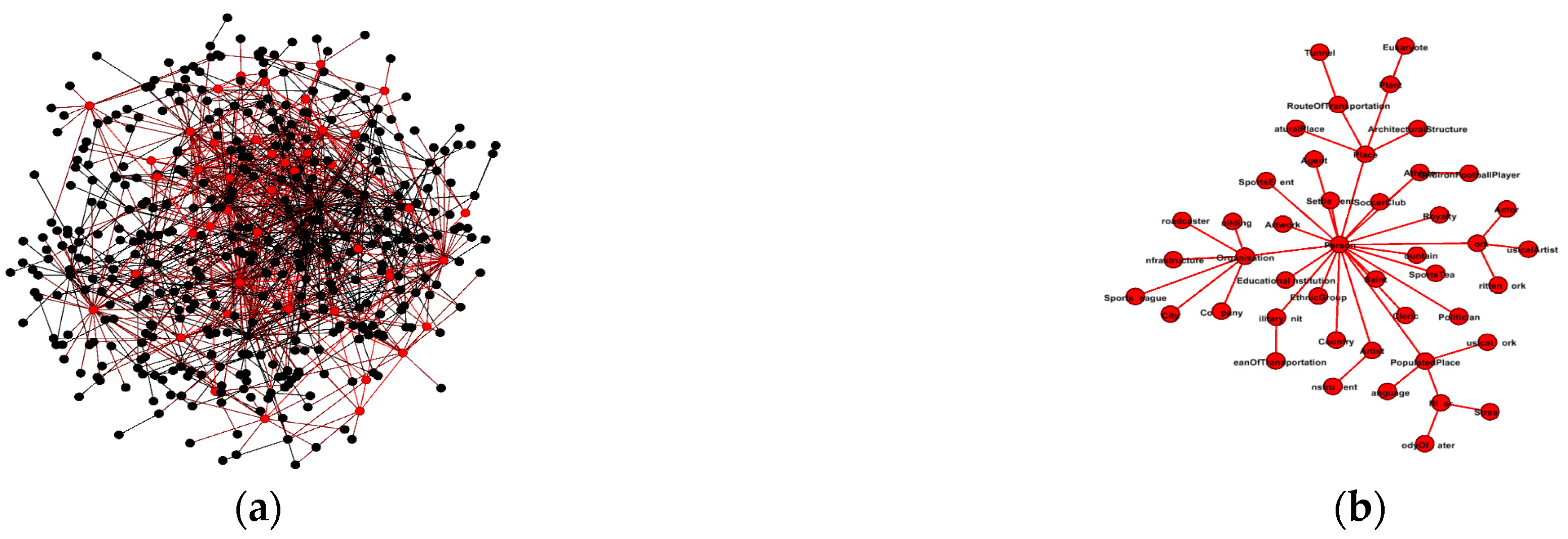
Example 1. Consider the DBpedia v3.8 which is shown in Figure 1a. Understanding the contents of the schema is difficult due to the numerous nodes available in the DBpedia schema graph. However, having a mechanism helping us to focus only on the most important subgraph it would allow us to get a quick overview of the contents of the KG. An example such summary is shown in Figure 1b. 4. Constructing Schema Summaries
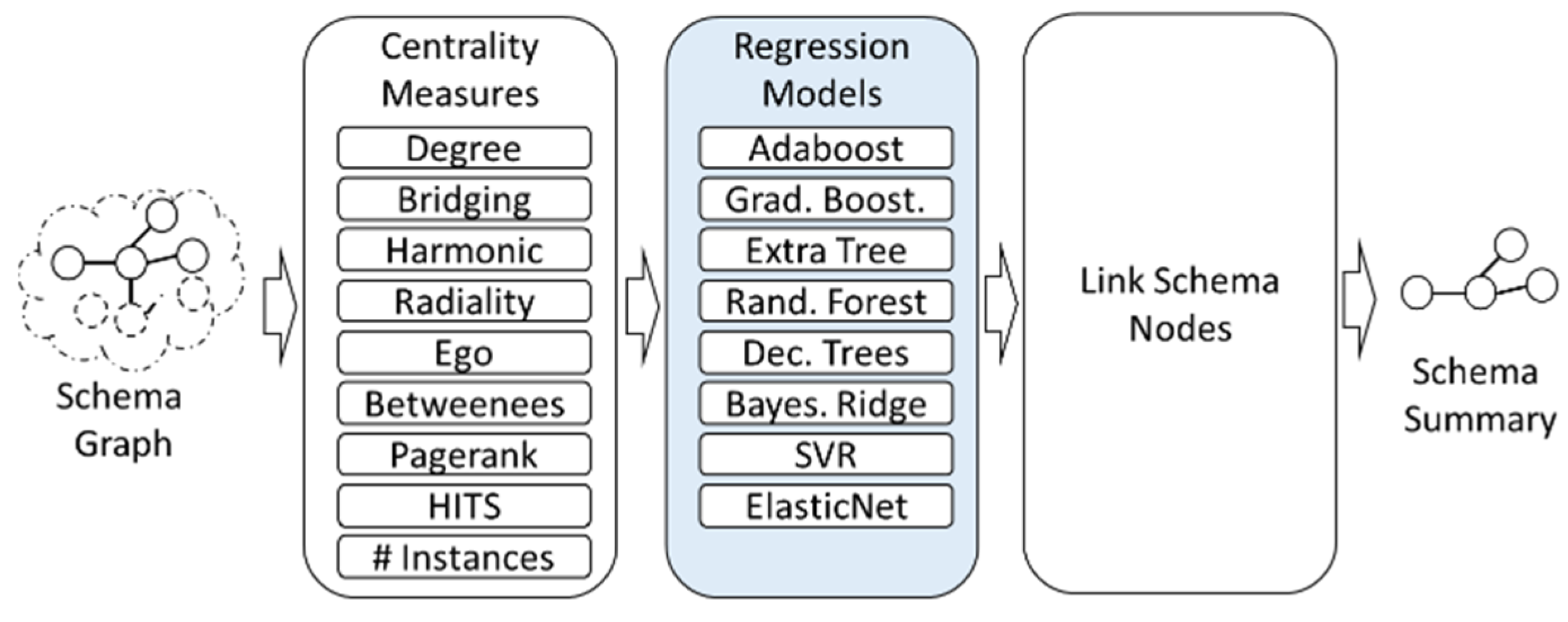
Our proposed system, named SumMER, employees a procedure of three steps for constructing a high quality structural semantic summary given an input RDF/S KG. In the first step SumMER is calculating eight centrality measure for each node. Then it uses those centralities for training/testing using eight diverse machine learning models. Finally, having selected the top-k schema nodes it links them and returns the generated summary to the user. The whole workflow is shown in
Figure 2.
More specifically, assuming that we have a function TOPk(GS) that for a given schema graph GS returns the k most important nodes, we define a summary schema graph of size k to be the following:
Definition 2. (Summary Schema Graph of size k). Let V = (GS, GI, λ, τc) be an RDFS KG. A summary schema graph of size k for V is a connected schema graph G′S = (V′S, E′S), G′S ⊆ Cl(GS), with:
V′S = TOPk(V) ∪ VADD, VADD represents the nodes in the summary used only to link the nodes in TOPk(V)
∀vi, vj ∈ TOPk(V), ∃ path(vi, vj) ∈ G′S,
there is no other summary schema graph G″S = (V″S, E″S) including the nodes in TOPk(V), such that, |V″S|<|V′S|.
In the sequel we describe each one of the steps shown in
Figure 2 in detail.
4.1. Computing Centrality Measures
Schema summarization aims to highlight the most representative concepts of a schema, preserving important information and reducing the size and complexity of the schema [
5]. Despite the significance of the problem, there is still no universally accepted measurement on the importance of nodes in an RDF/S graph. In this section, we describe eight alternative measures that have been proposed for capturing importance in directed graphs. We selected the Degree, the Betweenness, the Bridging Centrality, the Harmonic Centrality, the Radiality, the Ego Centrality and in addition HITS and PageRank as they constitute the state-of-the-art measures for generic graphs [
13]. The complexities of all measures are shown in
Table 1.
The simplest importance measure for a graph is the Degree (DE) that is defined as the number of edges incident to a node.
Definition 3. (Degree) Let GS = (VS, ES) be an RDF/S schema graph with vs. nodes and ES edges. The Degree of a node v ∈ vs. is the number of edges incident to the node.
The Betweenness (BE) measure is equal to the number of the shortest paths from all nodes to all others that pass through that node. Calculating the betweenness for all nodes in a graph requires the computation of the shortest paths between all nodes.
Definition 4. (Betweenness) Let GS = (VS, ES) be an RDF/S schema graph. The Betweenness of a node v ∈ vs. is defined as follows:where σst is the total number of shortest paths from node s to node t and σst(v) is the number of those paths that pass-through v, where s ≠ v ≠ t. The Bridging Centrality (BC) tries to identify the information flow and the topological locality of a node in a network. It is widely used for clustering or in order to identify the most critical points interrupting the information flow for network protection and robustness improvement purposes. A node with high Bridging Centrality is a node connecting densely connected components in a graph. The bridging centrality of a node is the product of the betweenness centrality and the bridging coefficient, which measures the global and local features of a node respectively.
Definition 5. (Bridging Centrality) Let GS = (VS, ES) be an RDF/S schema graph. The bridging centrality of a node v ∈ vs. is defined as follows:where BC(v) is the bridging coefficient of a node which determines how well the node is located between high degree nodes and BE(v) is the betweenness centrality. The bridging coefficient of a node v is defined:where DE(v) is the degree of node v, and N (v) is the set of its neighbors. The Harmonic Centrality (HC) is a modification of the Closeness, replacing the average distance with the harmonic mean of all distances, requiring again the computation of the shortest paths between all nodes.
Definition 6. (Harmonic Centrality) Let GS = (VS, ES) be an RDF/S schema graph. The Harmonic Centrality of a node v ∈ vs. is defined as follows: The Radiality (RA) was first proposed to provide information on how close a node is to all other nodes in a graph (i.e., the integration measure of a node to a graph). In order to compute the diameter of a graph we need to compute the shortest paths between all nodes.
Definition 7. (Radiality) Let GS = (VS, ES) be an RDF/S schema graph. The Radiality of a node v ∈ vs. is defined as:where ∆GS is the Diameter of graph Gs. For a node v, Ego Centrality (EC) is the induced subgraph of G, which contains v, its neighbors, and all the edges between them, trying to identify how important a node is to his neighborhood.
Definition 8. (Ego Centrality) Let GS = (VS, ES) be an RDF/S schema graph. The Ego Centrality of a node v ∈ GS is defined as followswhereand e.ego = 1/vιout, vi the adjacent node of a node v using the incoming edge e, e.ego = 1/vιin, vi the adjacent node of a node v using the outgoing edge e. The HITS (HT) algorithm [
14] is based on the idea that in the Web, and in all document collections which can be represented by directed networks, there are two types of important nodes: hubs and authorities. Hubs are nodes which point to many nodes of the type considered important. Authorities are these important nodes. For ranking schema nodes, we initialize every schema node with
auth(
v)
= 1 and
hub(
v)
= 1. For computing the hub and authority scores of every node, repeated iterations are applied. So, first the Authority Update Rule and then the Hub Update Rule is executed
k times.
Definition 9. (HITS) Let GS = (VS, ES) be an RDF/S schema graph. The hub and the authority of a node v ∈ vs. is defined as follows:where v is a schema node, Vto includes all schema nodes that link to the schema node v, and Vfrom includes all schema nodes to which the schema node v links. The final hub-authority scores of nodes are determined after infinite repetitions of the algorithm. The last important measure which was considered is the PageRank (PR) [
15] algorithm. PageRank assigns a score based on node’s connections and their connections. PageRank takes link direction and weight into account so links can only pass influence in one direction, and pass different amounts of influence
Definition 10. (PageRank) Let GS = (VS, ES) be an RDF/S schema graph. The PageRank of a node v ∈ vs. is defined as followswhere v is a schema node, Bv is the set that includes all schema nodes linking to v and L(v) is the number of links from the schema node v. 4.2. Selecting the Top-k Nodes as a Regression Problem
In this work, we argue that the various centralities offer complementary perspectives on assessing a node’s importance. As such we move beyond approaches that try to identify a single optimal measure (e.g., [
2,
4]). In order to combine multiple measures for selecting the k most important schema nodes we model the problem as a regression problem. The features of each schema node are the various centrality measures. In addition, we also add in the feature vector the normalized number of instances belonging to each schema node, as we believe that the more populated with instances a schema node is the most important should be. We explore eight ML regressor algorithms to this purpose: Adaboost (AB), Gradient Boosting (GB), Extreme Random Forest (ERF), Random Forest (RF), Decision Tree (DT), Bayesian Ridge (BR) and ElasticNet (EN).
Example 2. For our running example, the following table (Table 2) is constructed, including the features that will be given as input to the machine learning algorithms. All algorithms are quite efficient, in their test phase. The complexities of the algorithms are shown in
Table 3 [
16,
17]. Note that complexities depend on many factors, such as number of features, samples, number of trees, depth of the trees (e.g., for Random Forest), etc. Note also that Bayesian Ridge regressor and Elastic Net regressor are Linear regressors as well.
4.3. Linking Selected Schema Nodes
Assuming that the previous two steps were successful in selecting the most important nodes, next we focus on linking those nodes with appropriate paths out of the original schema graph to generate a sub-graph of it. The direction of the edges is irrelevant as we seed only to connect the selected schema nodes.
Past approaches in the area exploit the maximum-cost-spanning tree, linking the most important nodes using paths from the selected maximum-cost-spanning tree (MST) [
18]. The target in those approaches is to that maximize the total weight of the selected sub-graph. However, as the MST identifies the paths that maximize the weight for the whole graph, linking the top-k schema nodes using paths from the MST, introduces a significant number of additional nodes in the result summary highly reducing the value of the generated summary, as the new nodes might not have a high value.
In this paper, we model the problem of linking the most important nodes as a variation of the well-known graph Steiner-Tree problem (GSTP) pursuing a different optimization objective. To reduce the number of additional schema nodes introduced to the result summary.
Definition 11. (The Graph Steiner-Tree problem (GSTP)) Given an undirected graph G = (V, E), with edge weights and a node set S, called terminals, where S ⊆ V, find a minimum-weight tree T = (Vt, Et) ∈ G such that S ⊆ Vt and Et ⊆ E.
In our case, the graph given as input to the algorithm is the schema graph, ignoring the direction in the edges, as our target is to link the top-k nodes independent of the direction of the edges in between. Our objective now is not to increase the total weight of the summary graph but to introduce as less as possible additional nodes to the summary required for linking the top-k ones. This is since introducing a lot of additional nodes shifts the focus of the summary and decreases the summary’s quality. For resolving this problem optimal solutions have been already proposed by Hakimi [
19] and Levin [
20] independently. The problem is an NP-hard problem and remains NP-complete if all edge weights are equal.
Algorithms, Approximation & Heuristics
There had been various exact algorithms for the GSTP.
Hakimi [
19] proposed the first brute force, exact algorithm for resolving the GSTP problem. The algorithm enumerates all minimum spanning trees of sub-networks of
G included by super-sets of terminals that runs in
O(2
V−t V2 +
V3). The first dynamic programming algorithms were proposed independently by Dreyfus & Wagner [
21] and by Levin [
20]. The former runs in
O(3
t V + 2
t V2 +
V3) whereas the latter in
O(3
t V + 2
t V2 +
t2 V) and they are based on the optimal decomposition property by creating two node sets, removing one node at each step and solving the GSTP by connecting each set. Levin’s method uses a recursive optimization approach that pre-computes the possible sub-trees. Since all algorithms have an exponential running time, various approximations such as [
22,
23,
24] have been proposed in order to find good solutions for large networks. A central theme in these approximations is the use of some principles known from the two classic algorithms for solving the minimum spanning tree problem, Prim’s and Kruskal’s [
24]. We use the following top-three well-known and good performing methods SDISTG, CHINS and HEUM [
24]. These approximations have a worst-case bound of 2, i.e.,
ZT/Zopt ≤ 2·(1 −
l/|Q|), where
ZT and
Zopt denote the objective function values of a feasible solution and an optimal solution respectively,
Q the set of terminals and
l a constant [
25].
Besides these approximations, many heuristics can be employed to improve even more the corresponding algorithms. The most promising ones are the I-MST+P and the TRAFO [
24]. I-MST+P is a pruning routine that ensures that all leaves are terminal nodes whereas TRAFO transforms a feasible solution to another one trying to overcome the deficiency of bad local optima by allowing the temporary deterioration of the actual solutions. In this paper we use only the I-MST+P since TRAFO requires considerably more time to run and the improvements are insignificant—due to the sparsity of the examined ontologies.
Complexities Using a Breadth-first search (BFS) requires
O(
V +
E) time (where
E is
O(
V)) to find the shortest paths from a source vertex
v to all other vertices in the graph. All- pairs shortest paths for unweighted undirected graphs can be computed in
O(
V (
V +
E)) time by running the BFS algorithm for each node of the graph. The complexity of SDISTG, CHINS and HEUM differs, due to the usage of different heuristics.
Table 4 provides the worsts case complexity of those algorithms for weighted and unweighted graphs.
5. Evaluation
Next, we present in details the datasets used for our experimental evaluation and the methodology followed.
Datasets. As we shall show in the sequel, we exploit query logs for evaluating the quality of the summaries constructed. As such we can only use KGs where query logs are available. Three real world KG with such query logs available are DBpedia v3.8 and v3.9, and the Semantic Web Dog Food (SWDF) which we subsequently used. We could not identify other KGs with big query logs available online. Finally, although WikiData has such a query log available its huge size (more than 1.4 billion statements) does not allow schema extraction that would be used then for summarization and as such was not used in this paper. Nevertheless, we argue that three real world datasets with thousands of user queries are enough for evaluating our approach.
DBpedia v3.8 contains 315 classes, 1323 properties and more than 2.3 M instances, and DBpedia v3.9, contains 533 classes, 1805 properties and more than 3.3 M instances. The dataset occupies 103 GB of storage for v3.8 and 114 GB for v3.9. We had also available a query log with 50 K user queries for v3.8 and 110 K user queries for v3.9, as provided by the DBpedia SPARQL end-point. The v3.9 of DBpedia does not contain all samples of v3.8 since it was a major update, with many updates/deletions in the old triples, and the introduction of new ones. Although the two versions of the DBpedia are not the most recent ones, they have already proved their value in various benchmarks and experiments (e.g., [
26]) and give us an interesting dataset to experiment with, especially because we have also thousands of user queries available.
In addition, we used the Semantic Web Dog Food (SWDF) [
27]. SWDF is a KG containing information about semantic web conferences. Its schema contains 120 classes, 72 properties, 304,583 triples, 36,879 distinct subjects, 185 distinct predicates, and 95,501 distinct objects. The dataset occupies 50 MB of storage. For this dataset, we exploited also a query log containing 2.5 K user queries, provided by LSQ.
Table 5 presents the characteristics of the KGs used for our evaluation.
Constructing a “golden standard”. For constructing a “golden standard” to be used for the evaluation of the selection of the top-k nodes, we exploit the query logs available for the three KGs. More specifically, based on these query logs we calculate the frequencies of the schema nodes in the user queries. For calculating those frequencies, we are not considering only the direct appearances of the schema nodes in the queries but also include the appearance of the instances that they belong to those schema nodes. Using this frequency, we argue that the most important ones are the ones more frequently queried, a reasonable assumption as the more user queries involve a specific schema node the more important this node should be.
Certainly, if thousands of user queries were available for all KGs then we could construct an ideal summary for all of them, based exactly on the schema nodes that are most frequently queried. However, through our involvement in semantic summaries we soon realized that such query logs are available only for a limited set of cases, and methodologies like the one proposed in this paper are required to formulate high-quality summaries, even without the presence of those query logs.
5.1. Centrality Measures Correlation
In our first experiment, we explore the statistical dependence between the ranking of all nodes using the defined centrality measures and the number of instances and the golden standard ranking. We use Spearman’s rank correlation coefficient [
28] for assessing the strength and the direction of association between the golden standard ranking and each centrality measure.
Spearman correlation indicates the direction of the association between two variables X, Y. It varies between −1 and 1. 1 is a total positive correlation, 0 is no correlation, and −1 is a total negative correlation. If Y tends to decrease when X increases, the Spearman correlation coefficient is negative. A Spearman correlation of zero indicates that there is no tendency for Y to either increase or decrease when X in- creases. When X and Y are perfectly monotonically related, the Spearman correlation coefficient becomes 1.
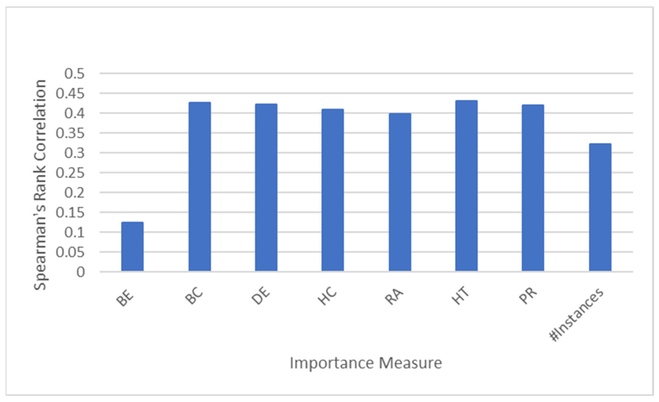
The results of our experiments are shown in
Figure 3. As shown, we can see a variation in the correlation depending on the importance, reaching a maximum of 0.44 correlation. As such we can easily conclude that no single centrality measure is enough to predict the most frequent schema nodes across the available.
5.2. Machine Learning for Schema Node Selection
Next, we focus on exploiting multiple importance measures for selecting schema nodes. For evaluating the performance of our ML algorithms, we use Mean Absolute Error (MAE), Root Mean Squared Error (RMSE) and Median Absolute Error (MedAE) as they are commonly used for evaluating regression problems [
29]. The
is the predicted value, y is the corresponding actual value and samples is the number of samples:
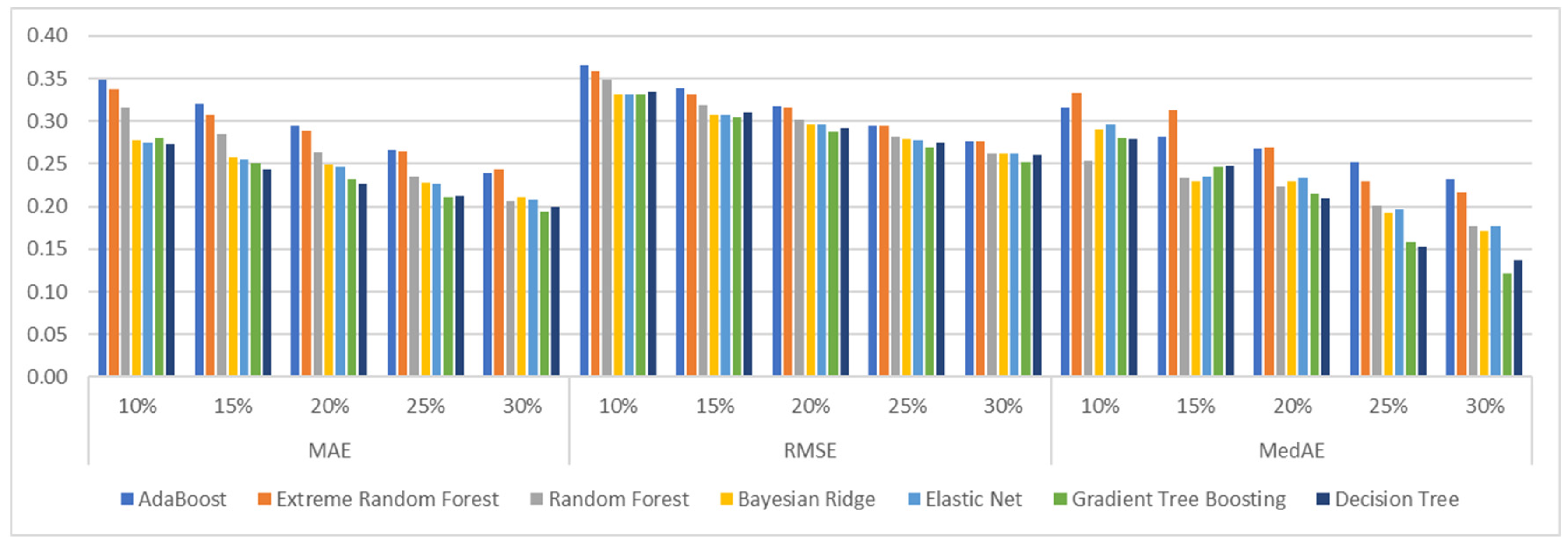
As we are only looking for the top-k nodes, we evaluate those metrics on the top-k nodes only. Further, we examine the performance of the ML algorithms on selecting the 10%, 15%, 20%, 25% and, 30% most important schema nodes out of the total schema nodes available in the dataset. We use the DBpedia v3.9 as the training dataset and the DBpedia v3.8 and SWDF as the test datasets.
DBpedia: The results for DBpedia v3.8 are shown in
Figure 4. In addition,
Table 6 shows part of the confusion matrix of the various algorithms for the selection of the 10%, 15%, 20%, 25%, 30% top nodes. As shown in
Figure 4, the Decision Tree regressor performs best in most of the cases, whereas most of the algorithms show a relatively good performance.
Table 6 presents a part of the confusion matrix where we can see the true positives (TPs) that the various ML algorithms predict. As shown Decision Tree regressor makes the best predictions on the true positives (TP) in most of the cases (10%, 15%, 20%, 25%, 30%). Adaboost Regressor has also a good performance in selecting the TPs however it is not the best performer overall as seen also in
Figure 4.
SWDF: The results for SWDF are shown in
Figure 5, whereas
Table 6 shows part of the confusion matrix of the various algorithms for the selection of the 10%, 15%, 20%, 25%, 30% top nodes. In this experiment, the Adaboost, Gradient Tree Boosting and Decision Trees regressors perform best in terms of MAE, MSE and Median Absolute Error, whereas looking in
Table 7 we can identify that Decision Tree Regressors performs also best in detecting the TPs. As the information provided in confusion matrices is only partial it is natural to see differences with the regression evaluation measures (MAE, MSE, Median Absolute Error)—regression measures compute the distance error for all the values while the confusion matrix computes only to miss or hit for the class.
Overall, we can easily see that the Decision Trees Regressor shows an excellent performance among the two datasets and can always make good predictions. As such for the rest of the evaluation we only include the Decision Tree Regressor. Finally, we have to note that the highest-ranked features from the Decision Tree regressor are Hits, PageRank and the number of instances.
5.3. Additional Nodes Introduced
As the Steiner-tree approximations we use also introduce new nodes in the generated summary next we focus on identifying the overhead introduced by that. More specifically,
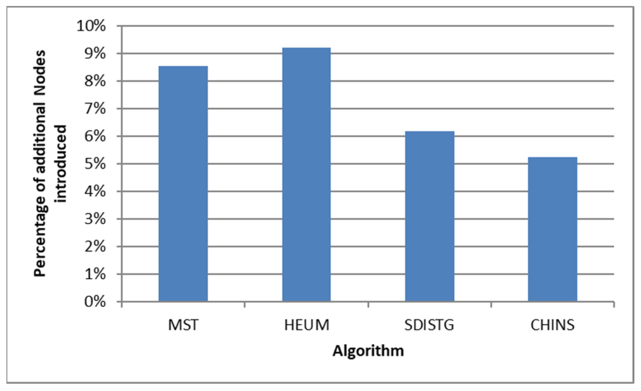
Figure 6 presents the percentage of the additional nodes introduced in the generated summary. In addition, we report the percentage of the additional nodes for the MST algorithm that has been used in the past. MST introduces on average 8.5%, HEUM 9.2%, SDISTG 6.2%, and finally CHINS 4.7% additional schema nodes. For DBpedia v3.8 this corresponds to 3 additional schema nodes in the case of MST contrasted to the 2 schema nodes introduced by CHINS (10% summary). This is reasonable since our Steiner-Tree approximations target specifically the minimization of the additional nodes introduced in the generated summary. Note also that not all approximations are equally beneficial, as the HEUM approximation is even worse than MST. Based on these results for the SumMER we only keep the CHINS approximations for the rest of the experiments.
5.4. Evaluating Summary Quality
Although measures like MAE, SMSE, and MedAE can effectively evaluate the regression models, they cannot completely evaluate the generated summaries overall. Also, these measures fail to identify the added value of a semantic summarization system when the results are not the same as the ones in the “golden standard”.
As such we exploit coverage, calculating for each query the percentage of the classes and properties that are included in the summary. Again, a class/property appears within a query either directly or indirectly. Directly when the specific class/property appears within a triple pattern of the query. Indirectly for a class is when the said class is the type of an instance or the domain/range of a property that appears in a triple pattern of the query. Indirectly for a property is when the said property is the type of an instance. Having the percentages of the classes and properties included in the summary, the query coverage is the weighted sum of these percentages. As our summaries are node-based we give 0.8 weight to the percentage of the classes and 0.2 weight to the percentage of the properties.
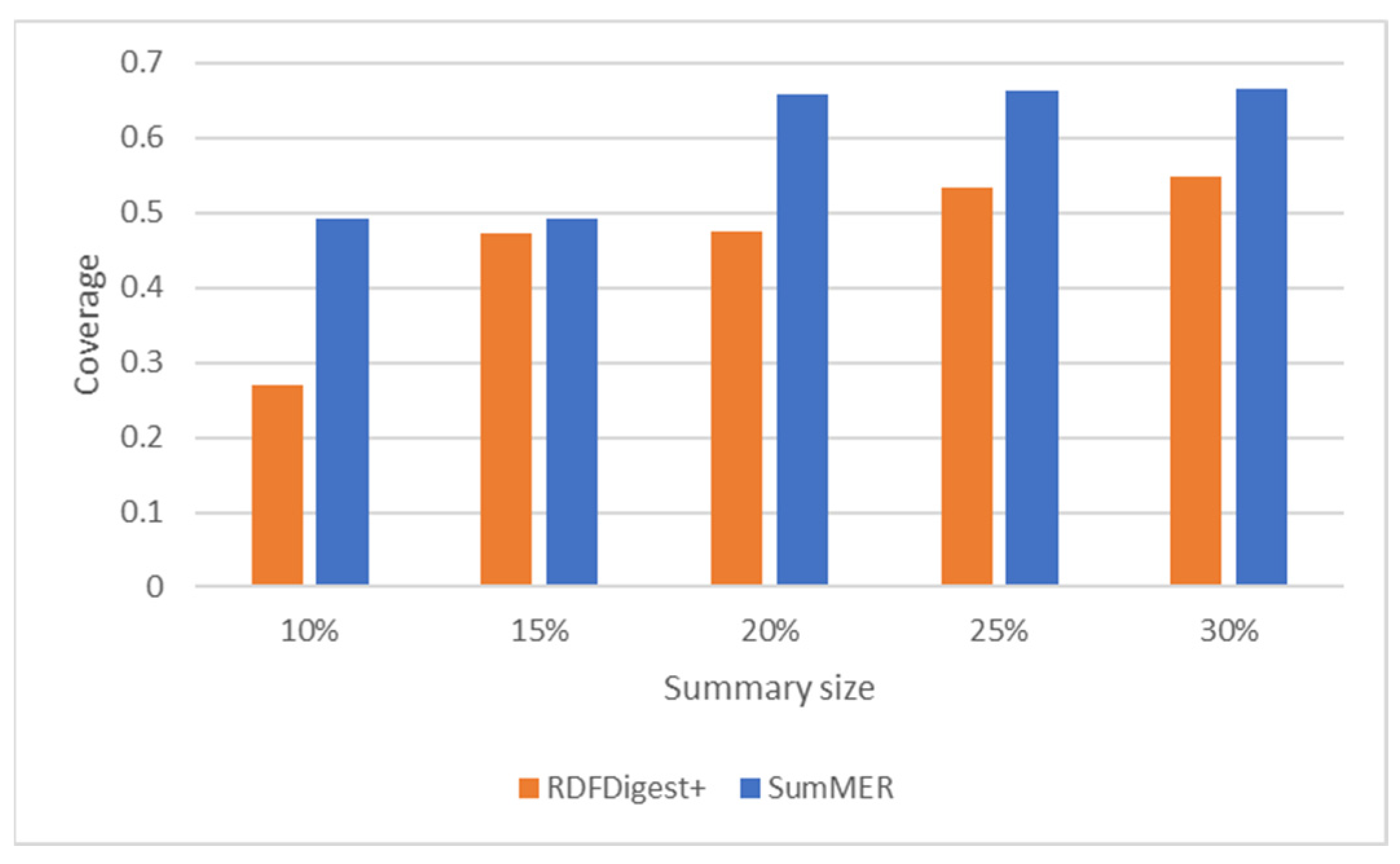
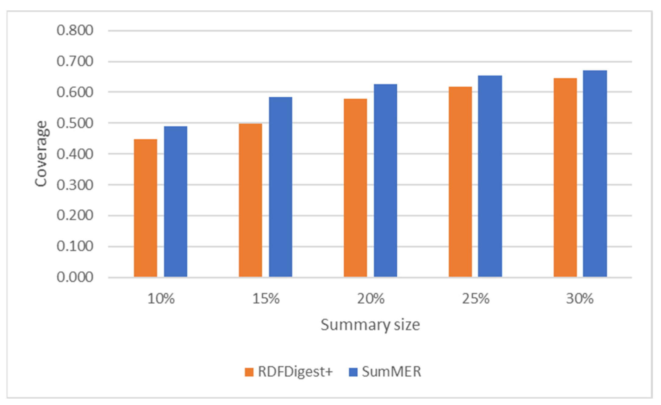
Definition 12. (Coverage). Let (VS, ES) be a KG GS, Q a query workload Q = {q1, …, qn}, and two weights for nodes and edges, i.e., wnodes and wprops. Query coverage is defined as follows: The results on summary quality based on coverage are shown in
Figure 7 for DBpedia v3.8, and in
Figure 8 for SWDF. We compare our results with the state-of-the-art system in structural semantic summaries RDFDigest+ [
6,
7]. RDFDigest+ employees an adaptation of the betweenness centrality for selecting the most important schema nodes, considering also the number of triples available for each class.
As shown, in both datasets SumMER can achieve a higher coverage than RDFDigest+ in all cases, always improving the coverage of the result summary.
Looking at the partial confusion matrix presented in
Table 8, we can identify that SumMER is able to make the best predictions on the TPs for all summary sizes, outperforming the RDFDigest+ in all cases. The improvement on the prediction of the top-k nodes is also depicted to the subsequent calculation of the query coverage for both DBpedia v3.8 and SWDF.
Overall, SumMER shows a stable performance, both in selecting the schema nodes and in the overall quality of the generated summary. As shown in our experiments SumMER generates better summaries, that can answer more query fragments than previous works. This happens not only for a different version of the same KG KG (DBpedia), but also for a completely different KG (SWDF), showing that our approach generalizes beyond the boundaries of the same KG.
5.5. Execution Time
Next, we evaluate the efficiency of the various components of our system. We present in each case the average time of 10 executions for summarizing the two KGs. All experiments ran on an Intel(R) CPU running at 2.70 GHz with 4GB memory on Windows 10.
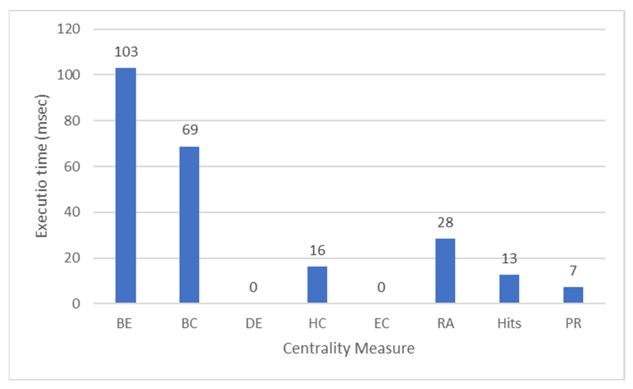
Calculating individual centrality measures. The average execution time for identifying the most important nodes on our largest test dataset (DBpedia v3.8) is shown in
Figure 9 for the various centrality measures.
As presented, the execution times are grouped into three categories. The ones that compute the shortest paths of all pairs, the ones that need to iterate only on the nodes and the edges of the graph and the ones that need to perform local iterations on the nodes and the edges. The Betweenness, the Bridging Centrality, the Harmonic Centrality and the Radiality belong to the first category. They all calculate the shortest paths between all pairs of nodes in order to assign the proper weights. As such, their execution time is similar. The Betweenness calculates the set of all shortest paths for all schema node pairs and as such it requires more time. The Bridging Centrality uses the Betweenness and as such, it takes almost the same time. In the second category, we have the Hits, PageRank, Degree, and the Ego Centrality. The Degree needs only to iterate over all edges of the graph and use this for the weight calculation for each node. The Ego Centrality requires one more iteration over all nodes and edges of the graph. As such they need only nanoseconds to be calculated for our graphs. In the third category, we find Hits and PageRank, where the weight of the edges is initialized, then the entire graph is crossed node by node, changing the corresponding weights and repeating the whole process.
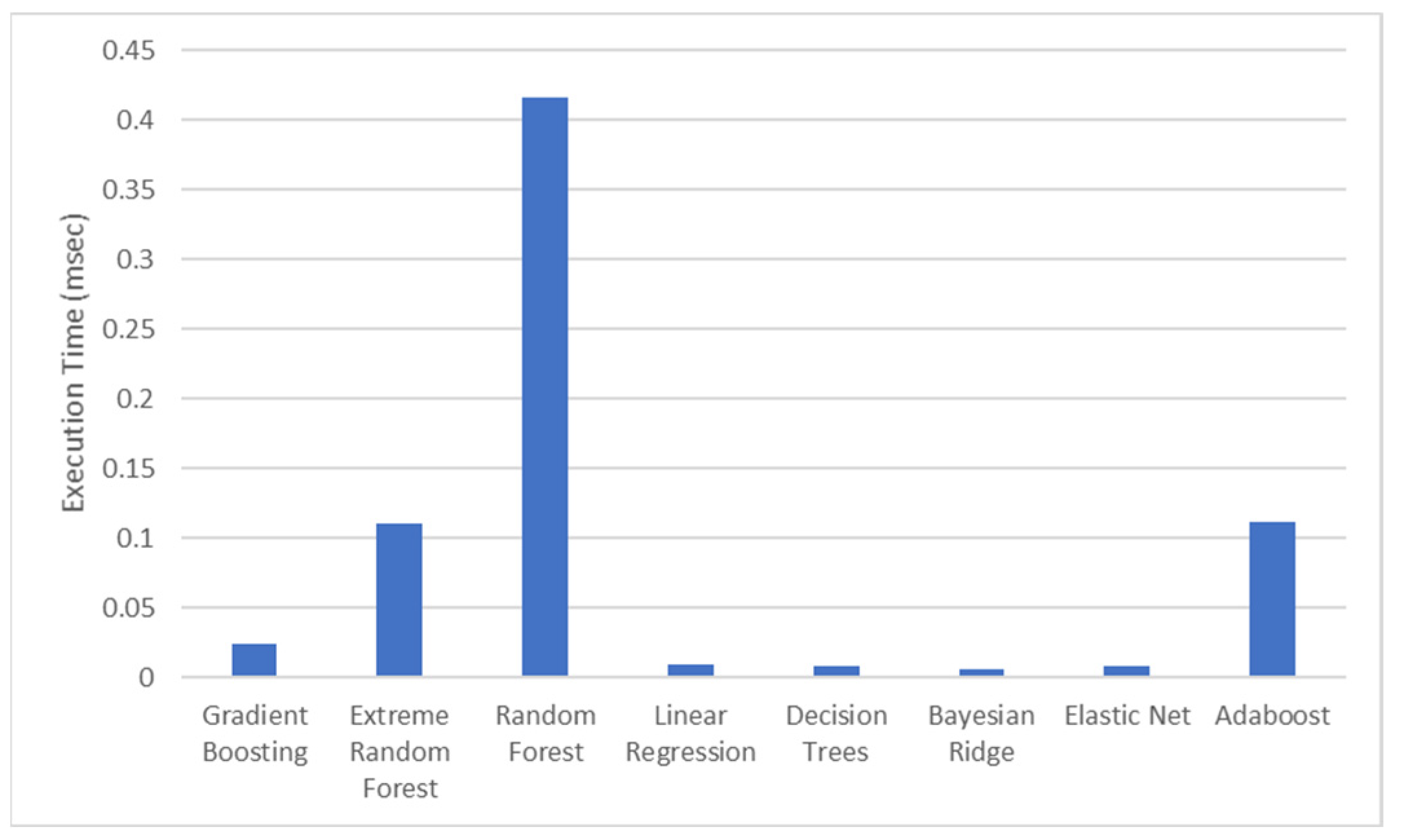
Using ML to calculate top-k nodes. The average execution times for the prediction of the most important nodes in our largest test dataset (DBpedia v3.8), are shown in
Figure 10. As shown, running the described machine learning algorithms is rapid fast, as those algorithms usually work with many more samples. More specifically, Linear Regressors (Linear Regression, Bayesian Ridge, and Elastic Net) and Decision Trees are the best performing ones, while Random Forest is the worst performing one. However, even the worst takes on average 0.4 msec to return the results. Those results are in line with the complexity of the corresponding algorithms already presented in
Section 4.2. Nevertheless, we can easily identify that the added overhead of the machine learning algorithms is negligible and we omit results for SWDF as the execution times are even smaller.
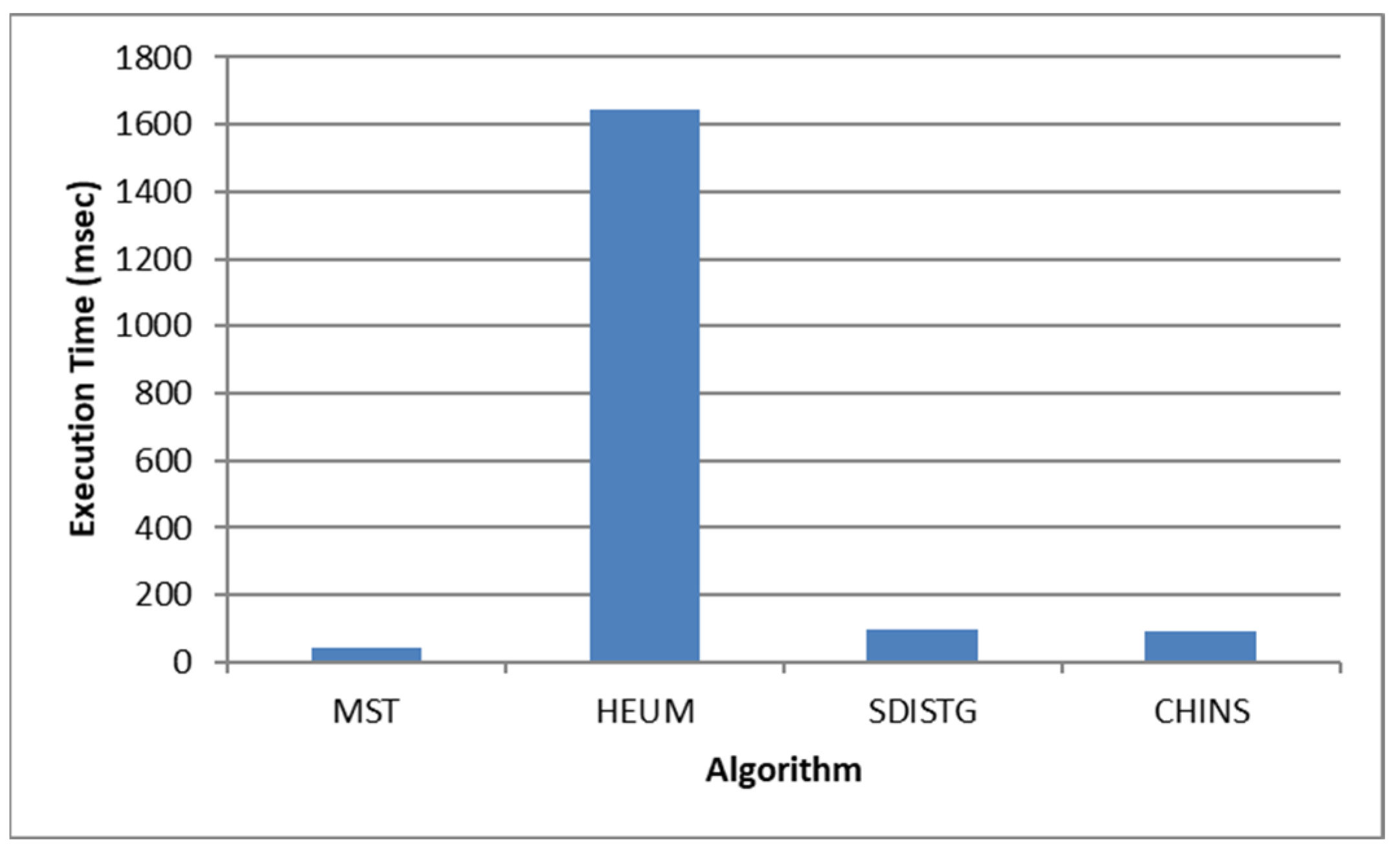
Linking top-k nodes. For linking the top-k schema nodes, according to the complexities of the corresponding algorithms, there is a linear functional relationship between the execution time and input data size for SDISTG and CHINS. The results are shown in
Figure 11. HEUM is requires a quadratic time, as it must construct the shortest paths of all pairs. Considering that the number of the selected schema nodes is relatively small SDISTG and CHINS have a better execution time. HEUM grows linearly to the number of nodes and performs worst. MST depends on the size of the graph and performs better than SDISTG and CHINS which are highly dependent on the number of the top-k schema nodes and the shortest paths between them.
6. Conclusions
In this paper, we present SumMER focusing on answering two key questions for constructing structural semantic summaries: (a) how to identify the most important nodes and (b) how to link the selected nodes in order to create a sub-graph of the original graph and return it to the user. For answering the first question we explore eight centrality measures for capturing nodes’ importance, and then, we effectively combine multiple of them, using machine learning techniques, transforming the selection of the k most important nodes out of an RDF/S KG into a regression problem. Subsequently, we implement three approximations of the graph Steiner-Tree problem for linking the selected nodes.
For our experimental evaluation we exploit query logs with numerous user queries, showing that machine learning has the potential to improve the quality of the generated summaries. Further after training, testing is practically rapidly fast. Overall, the Decision Tree regressor is the best performing algorithm showing a stability over the different KGs used. Further, the implemented Steiner-Tree approximations, introduce minimal nodes to the result schema graph. The best choice among the approximate algorithms is CHINS offering an optimal trade-off between quality and execution time.
Limitations. Although we have shown that SUMMER is able to generalize on another KG, further experiments are required for other KGs to identify that the results hold indeed in all other KGs. Unfortunately, KGs with available workloads are hard to find online. Another limitation of the current work is that our algorithms are focusing on the schema graph. Applying however our approach to the entire graph would require parallel implementation of the algorithms in this paper in order to finish in a reasonable time.
Future Work. As future work, our approach will be extended to handle constructs from OWL KGs such as class restrictions, disjointness and equivalences and explore other ML methods such as deep networks and methods for learning to rank [
30]. Further as KGs are not static but subject to continuous evolution summarizing different versions of the KGs and comparing those summaries would provide useful insights on how graphs evolve. Finally, it would be interesting to explore how Shapes Constraint Language (SHACL) [
31] expressions could be used instead our first level schema graph, in order to identify the structure of the underlying KG, and whether an additional abstraction step on top would lead to high-quality summaries.
