Abstract
We consider the problem of estimating tail probabilities of random sums of scale mixture of phase-type distributions—a class of distributions corresponding to random variables which can be represented as a product of a non-negative but otherwise arbitrary random variable with a phase-type random variable. Our motivation arises from applications in risk, queueing problems for estimating ruin probabilities, and waiting time distributions, respectively. Mixtures of distributions are flexible models and can be exploited in modelling non-life insurance loss amounts. Classical rare-event simulation algorithms cannot be implemented in this setting because these methods typically rely on the availability of the cumulative distribution function or the moment generating function, but these are difficult to compute or are not even available for the class of scale mixture of phase-type distributions. The contributions of this paper are that we address these issues by proposing alternative simulation methods for estimating tail probabilities of random sums of scale mixture of phase-type distributions which combine importance sampling and conditional Monte Carlo methods, showing the efficiency of the proposed estimators for a wide class of scaling distributions, and validating the empirical performance of the suggested methods via numerical experimentation.
1. Introduction
Tail probabilities of random sums have attracted the interest of researchers for decades, as they are important quantities in many fields; for instance:
- In insurance risk theory, these quantities correspond to the ruin probabilities associated with certain initial capital, and the random sum is a geometric sum of ladder heights (integrated tails of the claim sizes) in a claim surplus process; see, for example, [1].
- In queueing theory, stable single server Markovian queues with service times have a geometric length in equilibrium, and these quantities correspond to the probabilities that an arriving customer must wait longer than a certain time; see, for example, [2].
Estimation from sample data and density approximation with phase-type distributions was considered in [3], and parameter estimation for the class of discrete scaled phase-type distributions was subsequently treated in [4]. Maximum likelihood estimation via an expectation-maximisation (EM) algorithm was exploited in both papers.
Estimating tail probabilities of random sums has been extensively investigated both for light- and heavy-tailed summands. Classical methods, including large deviations, saddlepoint approximations, and exponential change of measure, are most commonly used. However, the application of these methods requires the existence of the moment generating function (MGF) of the summand, so are limited to light-tailed cases. In the heavy-tailed setting, subexponential theory provides asymptotic approximations but these offer poor accuracy for moderately large values ([5]). From a rare-event simulation perspective, there are a few efficient estimators proposed in the literature ([6,7,8]). Simulation methods for the heavy-tailed case often require the cumulative distribution function (CDF) or probability density function (PDF) of the summand, so these are frequently not easily implementable.
In this paper, we consider the problem of efficiently estimating the quantity
where , for large u. Specifically, N is a discrete light-tailed random variable supported over the positive integers and is independent of N and forms a sequence of independent, non-negative, and identically distributed random variables having stochastic representation where the random variables and are non-negative and independent of each other.
In our setting, the sequence belongs to the class of W-mixture of phase- type distributions (PH distributions), which can be represented as a product , where each is a non-negative but otherwise arbitrary random variable and is a PH-distributed random variable. The concept of W-mixture of PH distributions can be found in [9]. Bladt et al. [10] proposed a subclass of W-mixture of PH distributions to approximate any heavy-tailed distribution. Such a class is very attractive in stochastic modelling because it inherits many important properties of PH distributions—including being dense in the class of non-negative distributions and closed under finite convolutions—while it also circumvents the problem that individual PH distributions are light-tailed, implying that the tail behaviour of a heavy-tailed distribution cannot be captured correctly by PH distributions alone. Reference [11] showed that a distribution in the W-mixture of PH distributions class is heavy-tailed if and only if the random variable has unbounded support.
The CDF and PDF of a distribution in the W-mixture of PH distributions class are both available in closed form but these are given in terms of infinite dimensional matrices. The problem of approximating tail probabilities of scale mixture of PH-distributed random variables is not easily tractable from a computational perspective. Bladt et al. [10] addressed this issue and proposed a methodology which can be easily adapted to compute geometric random sums of scale mixture of PH distributions. Their approach is based on an infinite series representation of the tail probability of the geometric sum which can be computed to any desired precision at the cost of increased computational effort. In this paper, we explore an obvious alternative approach: rare-event estimation.
More precisely, we propose and analyse simulation methodologies to approximate the tail probabilities of a random sum of scale mixture of PH-distributed random variables. We remark that since the CDF and PDF of a distribution in the W-mixture of PH distributions class is effectively not available, most algorithms for the heavy-tailed setting discussed above cannot be implemented. Our approach is to use conditioning arguments and adapt the Asmussen–Kroese estimator proposed in [7]. The Asmussen–Kroese approach is usually not directly implementable in our setting because the CDF of the product is typically not available. We address this issue using a simple conditioning argument on either the PH random variable or the scaling random variable , thereby simply simulating the PH distribution and using the CDF of or simulating the scaling distribution and using the CDF of . Moreover, we explore the use of importance sampling (IS) on the last term of the summands.
The key contributions of this paper are as follows:
- Developing a number of rare event simulation methodologies;
- Proving the efficiency of proposed estimators under certain conditions;
- Exploring the proposed estimators through various numerical experiments.
The remainder of the paper is organised as follows. In Section 2, we provide background knowledge on PH distributions and scale mixture of PH distributions. In Section 3, we introduce the proposed algorithms. In Section 4, we prove the efficiency of the estimators proposed. In Section 5, we present the empirical results for several examples. Section 6 provides some concluding remarks and an outlook to future work.
2. Preliminaries
In this section, we provide a general overview of PH distributions and scale mixture of PH distributions.
2.1. Phase-Type Distributions and Properties
PH distributions have been used in stochastic modelling since being introduced in [12]. Apart from being mathematically tractable, PH distributions have the additional appealing feature of being dense in the class of non-negative distributions. That is, for any distribution on the positive real axis, there exists a sequence of PH distributions which converges weakly to the target distribution (see [2] for details). In other words, PH distributions may arbitrarily closely approximate any distribution with support on .
In order to define a PH distribution, we first consider a continuous-time Markov chain (CTMC) on the finite state space where states are transient and state ∆ is absorbing. Further, let the process have an initial probability of starting in any of the p transient phases given by the probability vector , with and . Hence, the process has an intensity matrix (or infinitesimal generator) Q of the form:
where T is a sub-intensity matrix of transition rates between the transient states, is a vector of transition rates to the absorbing state, and is a zero row vector.
The (continuous) PH distribution is the distribution of time until absorption of . The 2-tuple () completely specifies the PH distribution, and is called a PH-representation. The CDF is given by where is a column vector with all ones.
Besides being dense in the non-negative distributions, the class of continuous PH distributions forms the smallest family of distributions on which contains the point mass at zero and all exponential distributions, and is closed under finite mixtures, convolutions, and infinite mixtures (among other interesting properties) (see [12]).
2.2. Scale Mixture of Phase-Type Distributions
A random variable Z of the form is a scale mixture of PH-distributed if , where F is a PH distribution, and , where H is an arbitrary non-negative distribution. We call W the scaling random variable and H the scaling distribution. It follows that the CDF of Z can be written as the Mellin–Stieltjes convolution of the two non-negative distributions F and H:
The integral expression above is available in closed form in very few isolated cases. Thus, we should rely on numerical integration or simulation methods for its computation.
The key motivation for considering the class of scale mixture of PH distributions over the class of PH is that the latter class forms a subclass of light-tailed distributions while a distribution in the former class with scaling random variable having unbounded support is heavy-tailed ([11]). Hence, the class of scale mixture of PH distributions turns out to be an appealing tractable class for approximating heavy-tailed distributions. Recall that a non-negative random variable X has a heavy-tailed distribution if and only if equivalently, if Otherwise, we say X is light-tailed.
3. Simulation Methods
In this section, we introduce our rare-event simulation estimators for . The key approach is combining an Asmussen–Kroese-type algorithm with conditional Monte Carlo and further with importance sampling when necessary. The method is inspired by using the tower property of expectation where we have conditioned on some statistic T, and so in practical terms, one should be able to simulate T and compute .
3.1. Asmussen–Kroese-Type Algorithm
The Asmussen–Kroese estimator [7] is efficient for estimating tail probabilities of light-tailed random sums of heavy-tailed summands [13].
The key idea is based on the law of total probability and being the same for (as are i.i.d. random variables). We then have the following identity:
where is the complementary CDF of , , , and .
In our setting, the summands are heavy-tailed whenever has unbounded support [11] and so it is natural to consider this estimator here. Unfortunately, the Asmussen–Kroese approach is usually not directly implementable in our setting because the CDF of is typically unavailable.
Instead, we consider a simple modification, by conditioning on a single scaling random variable or on the PH random variable . We further consider applying a change of measure to this single random variable. Conditioning on N, the Asmussen–Kroese estimator (without applying the control variate method for N) for takes the form
In our context, when conditioning on the associated with , we arrive at
where is the complementary CDF of a PH random variable.
When conditioning on the XN associated with , we arrive at
where is the complementary CDF of a scaling random variable.
We then consider improving the efficiency of our algorithm by implementing IS over the distribution H or F, ensuring that the random sum after conditioning is equal in expectation to u. Inspired by popular methodologies drawn from light-tailed and heavy-tailed problems, we suggest two alternative approaches.
3.1.1. Exponential Twisting
The exponential twisting method is asymptotically optimal for tail probabilities of random sums with light-tailed summands ([14]).
Definition 1.
The estimator generated using the probability measure is said to be an asymptotically optimal estimator of if and only if
The method is specified as follows:
Define an exponential family of PDFs based on the original PDF of any random variable X, f, via
where is the MGF of X.
The likelihood ratio of a single element associated with this change of measure (i.e., using measure instead of ) is
where is the cumulant function of X. Then, the twisted mean is ([15]).
The selection of a proper twisting parameter is a key aspect in the implementation of this method. For dealing with the random sum (1), we select the twisting parameter such that the changed mean of the random sum is equal to the threshold, that is, . Note that .
For the case of conditioning on light-tailed scaling random variables, we combine the estimator (3) with the above importance sampling method, and arrive at the following estimator for a single replicate:
where is a generic copy of the scaling random variable, and h is the PDF of .
We further combine the estimators (3) and (5) with a control variate for N to improve the efficiency, which is based on the subexponential asymptotics :
For the case of conditioning on the PH random variables, we combine the estimator (4) with the above importance sampling method for both light- and heavy-tailed scaling distributions, and arrive at the following estimator for a single replicate:
where is a generic copy of the PH random variable, and f is the PDF of .
3.1.2. Hazard Rate Twisting
In this section, we consider the case in which scaling distributions are heavy-tailed. Writing the PDF of the scaling random variable W as h, its hazard rate is denoted by . Let denote the hazard function. Reference [8] introduced hazard rate twisting and the hazard rate twisted density with parameter , :
where , which is the normalisation constant. The resulting twisted PDF is
where .
The following equation will later be useful to compute the twisted tail probability:
Thus, conditioning on , and taking in to account , the likelihood ratio of a single element associated with this change of measure is
where .
Combining the estimator (3) with the above importance sampling method for heavy-tailed scaling distributions, we then arrive at the following estimator for a single replicate:
Since N is random, we combine the estimator above with a control variable, and this yields the estimator:
Note that Equations (12) and (13) have the same form as Equations (6) and (7), respectively. When we combine with the importance sampling method in this section, we exploit the hazard rate twisting method instead of the exponential twisting method.
Conditional (either on or on ) Asmussen–Kroese with importance sampling and control variate results are summarised in Algorithms 1 and 2 used to generate a single replicate.
Note that we replace u by when determining , since we perform change of measure only on .
| Algorithm 1 Conditional (on ) Asmussen–Kroese with importance sampling and control variate algorithm |
|
| Algorithm 2 Conditional (on ) Asmussen–Kroese with importance sampling and control variate algorithm |
|
4. Efficiency of the Modified Amussen–Kroese Estimator
In this section, we investigate the asymptotic relative error of the estimators . Since , the estimator is consistent and we have the following second-order efficiency measures (see [15]),
- 1.
- The estimator is said to be logarithmically efficient if the following condition on the logarithmic rates holds:
- 2.
- The estimator is said to have bounded relative error ifwhere K is a constant that does not depend on u.
- 3.
- The estimator is said to have (asymptotically) vanishing relative error if
We focus on subexponential distributions and related distributions. The definitions of these relevant distributions are listed as follows.
Definition 2.
A distribution function F with support on is subexponential, if , it satisfies
where denotes the n-fold convolution of . Denote the class of subexponential distribution functions by .
Definition 3.
A distribution function F with support on is dominatedly varying, if , it satisfies
Denote the class of dominatedly varying distribution functions by .
Definition 4.
A distribution function F with support on is long-tailed, if , it satisfies
Denote the class of long-tailed distribution functions by .
We also exploit the definitions of Weibullian tail from [16].
Definition 5
([16]). A distribution F on is said to have a Weibullian tail
We write if Z satisfies Definition 5.
The following examples are two examples of widely used distributions that have Weibullian tails.
Example 1.
The CDF of a Weibull distribution with shape parameter b and scale parameter a is
denoted as Weibull(b, a), and .
Example 2.
The asymptotic form of the tail of a general PH distribution has the form
where and (cf. [1]), so that we can write .
Lemma 1 in [16] provides the way to calculate the parameters of product of two random variables having Weibullian tails.
Lemma 1
([16]). Let , be independent non-negative random variables. Then, with
- ,
- ,
- .
Suppose that we have the following conditions for the random variables involved.
Condition 1.
Assume that N is an integer-valued random variable with and is a sequence of i.i.d. random variables with continuous distribution function , independent of N.
Condition 2.
There exists a function that satisfies one of the following:
- (1)
- almost surely;
- (2)
- .
Condition 3.
There exists a random variable U with , such that for all ,
almost surely.
Lemma 2.
If Condition 2 (1) and Condition 3 are fulfilled, we obtain
If Condition 2 (2) and Condition 3 are fulfilled, we obtain
Proof.
If Condition 3 is fulfilled, by dominated convergence, we then interchange limit and expectation in (16) to obtain the result. □
Note that if Condition 1 is fulfilled, then (14) is bounded.
We list the conditions and lemma above which are mirrored from [13] for the reader’s convenience.
Proposition 1.
The estimators and
- Have bounded relative error when N is light-tailed, and ;
- Are logarithmically efficient when N is deterministic, and W has a Weibullian tail with shape parameter .
Proof.
Based on the law of total variance , we can conclude that the conditional Monte Carlo estimator has lower variance than the estimator Y. Thus, we can obtain and for conditional Asmussen–Kroese estimators and .
The Asmussen–Kroese estimator (2) was proven to be logarithmically efficient when Z has a Weibullian tail in [7], and to have bounded relative error in [13] for the following three cases:
- N is light-tailed, and .
- N is light-tailed, and .
- N is bounded, and Z is Weibull-distributed with shape parameter .
Here, we extended the result to scaling random variables in similar cases for the estimators and , which are as follows:
- As a consequence of Corollary 3.3 in [17], if F is a non-degenerate phase-type distribution, and the scaling distribution , then the phase-type scale mixture distribution . Therefore, the estimators and attain the same efficiency as the Asmussen–Kroese estimator, as they have lower variance.
- By Lemma 1, we observe that a phase-type distribution has a Weibullian tail with shape parameter being 1, and if the scaling random variable , then . Furthermore, the shape parameter of Z is ; thus, Z is heavy-tailed.In [7], the authors restricted to the Weibull-type distribution with shape parameter in and showed that the Asmussen–Kroese estimator is logarithmically efficient when N is deterministic. By Lemma 1, we obtain that if the shape parameter of the scaling random variable , then the shape parameter of the phase-type scale mixture distribution is . Therefore, the estimators and attain the same efficiency as the Asmussen–Kroese estimator if the scaling random variable with .
□
Further combining with a control variate for the number of summands N will additionally improve the efficiency of the estimators and .
5. Numerical Experiments
In this section, we provide a variety of numerical experiments to illustrate the proposed simulation methods. In all illustrative cases, we consider each scaling random variable to have support on all of and each to be Erlang-distributed with shape parameter being k and rate parameter being . Erlang distributions are selected as an example PH distribution because they play an important role in the class of PH distributions ([18]). The class of generalised Erlang distributions (a series of k exponentials with their own rates where ) is dense in the set of all probability distributions on the non-negative half-line.
We remind the reader that in all cases, the resulting product is heavy-tailed since the scaling random variable has unbounded support.
We explore the estimators which are the conditional Asmussen–Kroese estimator with control variates for the number of summands, and the estimators and , which are the conditional Asmussen–Kroese estimator with importance sampling on the last term of the summands and control variate for the number of summands.
The figures we include in this paper are the estimates of for u in the range , empirical logarithmic rates obtained by estimating , and empirical relative errors obtained by estimating .
We explore the estimators combined with control variates for the number of summands to the exclusion of the estimators not combined with control variates in later examples, because combining with control variates will slightly improve the efficiency of the proposed estimators. We provide a preliminary comparison for the estimators , , and for the scaling random variable being exponential, and the estimators , , and for the scaling random variable being Weibull, aiming to rule out estimators that do not perform well in later examples. The details of density selection regarding importance sampling for the preliminary examples are discussed in Examples 3 and 4, and the results are summarised in Figure 1 and Figure 2, respectively. We observe that in Figure 1, estimators and perform poorly due to numerical instability. When u exceeds around 2600, it is beyond the capability of data calculation. Thus, we do not include the estimators and in later examples. In Figure 2, all estimators appear to provide sharp estimates. We also observe that the empirical logarithmic rate tends to 1 when u gets large, which suggests that the estimators are logarithmically efficient. Nevertheless, the empirical relative errors for the estimators without importance sampling is increasing and not as stable when u becomes large. Since we could observe a slight improvement when combining with control variates from both Figure 1 and Figure 2, we include the estimators combined with control variates exclusively.
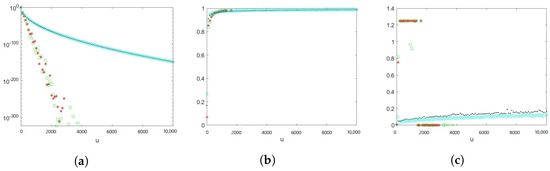
Figure 1.
The random variable N is geometrically distributed with success probability , , , where . Green circles: ConAK1. Red stars: ConAK1+CV. Black dots: ConAK1+IS (conditioning and IS on exponential). Cyan diamonds: ConAK1+IS+CV (conditioning and IS on exponential). (a) Estimates of as a function of u on a logarithmic scale. (b) Empirical logarithmic rates as a function of u. (c) Empirical relative errors as a function of u.
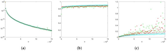
Figure 2.
The random variable N is geometrically distributed with success probability , , , where . Green circles: ConAK2. Red stars: ConAK2+CV. Black dots: ConAK2+IS (conditioning and IS on Erlang using an exponential PDF). Cyan diamonds: ConAK2+IS+CV (conditioning and IS on Erlang using an exponential PDF). (a) Estimates of as a function of u on a logarithmic scale. (b) Empirical logarithmic rates as a function of u. (c) Empirical relative errors as a function of u.
Example 3
(Light-tailed Scaling: Exponential). Let be the scaling random variable, with PDF
and consider , with PDF
where .
The Erlang distribution is the same as a gamma distribution with the shape parameter being an integer.
- (1)
- When conditioning on the scaling random variable, the resulting exponentially-twisted PDF iswhere . Hence, the likelihood ratio is given byThe choice of , conditioning on N, is determined by solving using , resulting in , and . The likelihood ratio for (7), conditioning on N, is given by
- (2)
- When conditioning on the PH random variable, the resulting PDF of the Erlang random variable is . Then, the likelihood ratio is given byWe solve using , conditioning on N, resulting in , and . The likelihood ratio for (10), conditioning on N, is given byAn alternative option is to perform importance sampling using the exponential PDF. Then, the likelihood ratio is given byWe solve using , conditioning on N, resulting in , and . The likelihood ratio for (10), conditioning on N, is given by
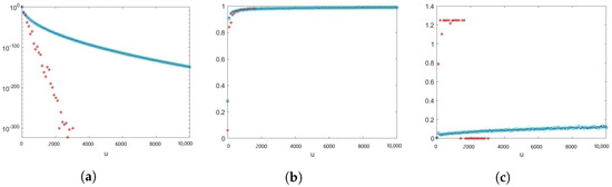
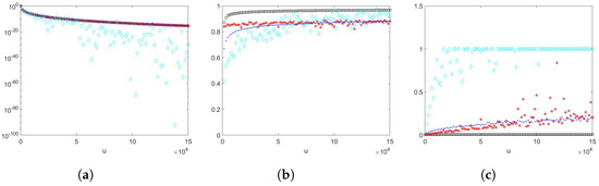
We take a sample size of , , , where and with , , , and . The results are shown in Figure 3. Proposition 1 does not provide a theoretical efficiency guarantee for this example as the number of summands is random, although the scaling random variable has a Weibullian tail. From numerical example results, we can observe that estimator is not providing reliable estimates; however, estimators and perform better.
Figure 3.
The random variable N is geometrically distributed with success probability , , , where . Black squares: ConAK1+IS+CV (conditioning and IS on exponential). Red stars: ConAK2+CV. Blue dots: ConAK2+IS+CV (conditioning and IS on Erlang using an exponential PDF). Cyan diamonds: ConAK2+IS+CV (conditioning and IS on Erlang using an Erlang PDF). (a) Estimates of as a function of u on a logarithmic scale. (b) Empirical logarithmic rates as a function of u. (c) Empirical relative errors as a function of u.
Example 4
(Heavy-tailed Scaling: Weibull). Let the scaling random variable be Weibull-distributed, with PDF
and consider , where .
- (1)
- When conditioning on the scaling random variable, the resulting hazard-rate twisted PDF of the scaling random variable isThus, conditioning on N, and taking into account , the likelihood ratio of a single element associated with this change of measure is
- (2)
- When conditioning on the PH random variable, the resulting PDF of the Erlang random variable is ; then, the likelihood ratio is given byWe solve using , conditioning on N, resulting in , and . The likelihood ratio for (10), conditioning on N, is given byAn alternative option is to perform importance sampling using the exponential PDF. Then, the likelihood ratio is given byWe solve using , conditioning on N, resulting in , and . The likelihood ratio for (10), conditioning on N, is given by
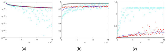
We take a sample size of , , , where , and with scale parameter , shape parameter , , , and . The results are shown in Figure 4. Proposition 1 does not provide a theoretical efficiency guarantee for this example as the number of summands is random, although the scaling random variable has a Weibullian tail. From numerical example results, we can observe that estimators and (importance sampling density using an exponential PDF) perform well. However, estimators and (importance sampling density using an Erlang PDF) appear to fluctuate more when u becomes larger, and they have increasing empirical relative errors.
Figure 4.
The random variable N is geometrically distributed with success probability , , , where . Black squares: ConAK1+IS+CV (conditioning and IS on Weibull). Red stars: ConAK2+CV (conditioning on Erlang). Blue dots: ConAK2+IS+CV (conditioning and IS on Erlang using an exponential PDF). Cyan diamonds: ConAK2+IS+CV (conditioning and IS on Erlang using an Erlang PDF). (a) Estimates of as a function of u on a logarithmic scale. (b) Empirical logarithmic rates as a function of u. (c) Empirical relative errors as a function of u.
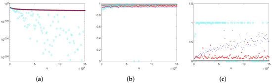
Next, we change random variable N from geometrically distributed to deterministic, and keep the rest of the parameters the same as above. The results are shown in Figure 5. Proposition 1 suggests that the estimator is logarithmically efficient as this example satisfies the second case of Proposition 1. From numerical example results, we can observe that estimators and (importance sampling density using an exponential PDF) perform well. However, estimators and (importance sampling density using an Erlang PDF) appear to fluctuate more when u becomes larger, and they have increasing empirical relative errors.
Figure 5.
The number of summands , , , where . Black squares: ConAK1+IS+CV (conditioning and IS on Weibull). Red stars: ConAK2+CV (conditioning on Erlang). Blue dots: ConAK2+IS+CV (conditioning and IS on Erlang using an exponential PDF). Cyan diamonds: ConAK2+IS+CV (conditioning and IS on Erlang using an Erlang PDF). (a) Estimates of as a function of u on a logarithmic scale. (b) Empirical logarithmic rates as a function of u. (c) Empirical relative errors as a function of u.
Example 5
(Heavy-tailed Scaling: Pareto). Let the scaling random variable be Pareto-distributed, with PDF
and consider , where . Note that Pareto distributions ; see [5].
- (1)
- When conditioning on the scaling random variable, the resulting hazard-rate twisted PDF of the scaling random variable isHence, the likelihood ratio is given byThus, conditioning on N, we set . Since in this case, the likelihood ratio of single element for (7), conditioning on N, is
- (2)
- When conditioning on the PH random variable, the resulting PDF of the Erlang random variable is ; then, the likelihood ratio is given byWe solve using , conditioning on N, resulting in , and . The likelihood ratio for (10), conditioning on N, is given byAn alternative option is to perform importance sampling using the exponential PDF. Then, the likelihood ratio for is given byWe solve using , conditioning on N, resulting in , and . The likelihood ratio for (10), conditioning on N, is given by
We take a sample size of , , , where , and with , , , and . The results are shown in Figure 6. Proposition 1 suggests that the estimator will have bounded relative error, since . From numerical example results, we can observe that the estimator performs well. The estimator has a few larger empirical relative error estimates as u is varied. Estimators (importance sampling density using an Erlang PDF and using an exponential PDF) appear to fluctuate more when u becomes larger, and they have increasing empirical relative errors.
Figure 6.
The random variable N is geometrically distributed with success probability , , , where . Black squares: ConAK1+IS+CV (conditioning and IS on Pareto). Red stars: ConAK2+CV (conditioning on Erlang). Blue dots: ConAK2+IS+CV (conditioning and IS on Erlang using an exponential PDF). Cyan diamonds: ConAK2+IS+CV (conditioning and IS on Erlang using an Erlang PDF). (a) Estimates of as a function of u on a logarithmic scale. (b) Empirical logarithmic rates as a function of u. (c) Empirical relative errors as a function of u.
Example 6
(Heavy-tailed Scaling: Log-normal). Consider now , and the scaling random variable with PDF
with corresponding CDF
where , and is the CDF of a standard normal random variate.
- (1)
- When conditioning on the scaling random variable, the resulting hazard-rate twisted PDF of the scaling random variable isThe likelihood ratio is given bywhere . The likelihood ratio for (7), conditioning on N, is given bywhere .We note that from (11), we have , and so it is straightforward to generate the twisted scaling random variables by using the inverse transform method.
- (2)
- When conditioning on the PH random variable, the resulting PDF of the Erlang random variable is ; then, the likelihood ratio is given byWe solve using , conditioning on N, resulting in , and . The likelihood ratio for (10), conditioning on N, is given byAn alternative option is to perform importance sampling using the exponential PDF. Then, the likelihood ratio is given byWe solve using , conditioning on N, resulting in , and . The likelihood ratio for (10), conditioning on N, is given by
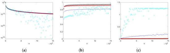
We take a sample size of , , , where , and with , , , , and . The results are shown in Figure 7. Proposition 1 does not provide a theoretical efficiency guarantee for this example as the log-normal distribution is neither nor has a Weibullian tail. From numerical example results, we can observe that estimators , , and (importance sampling density using an exponential PDF) perform well. (importance sampling density using an exponential PDF) turns out to have slightly lower empirical logarithmic rates and higher empirical relative errors than estimators and . The estimator (importance sampling density using an Erlang PDF) appears to fluctuate more when u becomes larger, and it has increasing empirical relative errors.
Figure 7.
The random variable N is geometrically distributed with success probability , , , where . Black squares: ConAK1+IS+CV (conditioning and IS on log-normal). Red stars: ConAK2+CV (conditioning on Erlang). Blue dots: ConAK2+IS+CV (conditioning and IS on Erlang using an exponential PDF). Cyan diamonds: ConAK2+IS+CV (conditioning and IS on Erlang using an Erlang PDF). (a) Estimates of as a function of u on a logarithmic scale. (b) Empirical logarithmic rates as a function of u. (c) Empirical relative errors as a function of u.
6. Discussion and Outlook
In this paper, we proposed straightforward simulation methods for estimating tail probabilities of random sums of scale mixture of PH-distributed summands. We combined Asmussen–Kroese estimation with the conditional Monte Carlo method and further exploited importance sampling applied to the last term of the summands. Since the method can perform poorly when the number of summands is large, we implemented an additional control variate for N to improve the accuracy of this estimator.
When combining Asmussen–Kroese estimation with the conditional Monte Carlo method, we can either condition on the scaling random variable or PH random variable. The estimators are denoted as and , respectively. In the given examples, we compared the estimators , , (importance sampling using an exponential PDF), and (importance sampling using an Erlang PDF). We took the distribution of N to be geometrically distributed in most cases, with one extra example for N as deterministic.
We observed that in Example 3, where the scaling random variable was exponentially distributed, the estimators and with importance sampling density being either exponential or Erlang gave sharp estimates and empirical logarithmic rates which tended to 1 as u became large, and also had lower empirical relative errors than estimator . The estimator performed poorly due to the calculation capacity issue, as we observed that when u exceeded around 1500, the empirical relative errors were 0 in Figure 3c. The poor performance of estimator is not surprising as Proposition 1 does not provide theoretical efficiency guarantees when the scaling random variable has a Weibullian tail and the number of summands is random.
In Example 4, where the scaling random variable was Weibull-distributed, we took the number of summands N being geometrically distributed or being deterministic. The results are summarised in Figure 4 and Figure 5. We observed that all the estimators in both examples performed similar. The estimators , , and (importance sampling using an exponential PDF) gave sharp estimates and empirical logarithmic rates which tended to 1 as u became large, and also had lower empirical relative errors than estimator with importance sampling density being Erlang. Despite positive indications from the empirical logarithmic efficiency estimates, the empirical relative errors for the estimator had an increasing trend and were fluctuating. Among the other two better-performing estimators, the estimator had the lowest empirical relative errors, and empirical logarithmic rates which tended to 1 faster.
In Example 5, where the scaling random variable was Pareto-distributed, the estimators , , and (importance sampling using an exponential PDF) gave sharp estimates and empirical logarithmic rates which tended to 1 as u became large, and also had lower empirical relative errors than estimator with importance sampling density being Erlang. Despite positive indications from the empirical logarithmic efficiency estimates, the empirical relative errors for the estimator (importance sampling using an exponential PDF) had an increasing trend and were fluctuating. Among the other two better-performing estimators, the estimator had the lowest empirical relative errors, and empirical logarithmic rates which tended to 1 faster.
In Example 6, where the scaling random variable was log-normal-distributed, we observed similar trends as in Example 5. In this example, we observed that the estimators , , and (importance sampling using an exponential PDF) gave sharp estimates. Empirical logarithmic rates of all the estimators appeared to tend to 1 as u became large. The estimators , , and (importance sampling using an exponential PDF) had lower empirical relative errors than estimator with importance sampling density being Erlang. The estimators and performed similarly, and showed better performance with empirical relative errors closer to 0, and higher empirical logarithmic rates in this example.
In all the above examples, the estimator (importance sampling using an exponential PDF) appeared to perform better than the estimator (importance sampling using an Erlang PDF), with sharp estimates, empirical logarithmic rates closer to 1, and lower empirical relative errors.
Finally, the examples given suggest that the estimator performs well when the scaling random variable has a heavier tail. The efficiency study suggests that and will attain the same efficiency as the Asmussen–Kroese estimator for the classes of distributions in Proposition 1. However, when conditioning on the scaling random variable, we do not always obtain reliable estimates due to the numerical limitations. In this case, the numerical experiments suggest that further exploiting importance sampling on the scaling random variable of the last term of the summands will provide more reliable estimates. For the log-normal case which does not fall in the cases in Proposition 1, we do not apply Proposition 1 to conclude theoretical efficiency for the scaling random variable being log-normal-distributed. However, the numerical experiment suggests that the estimator performs the best.
In conclusion, numerical studies suggest that, in general, the estimator will provide more reliable estimates when estimating tail probabilities of random sums of PH scale mixture random variables. When the scaling random variables have much heavier tail (e.g., log-normal case), the estimator performs better than in other cases. For all cases, the estimator (importance sampling using an exponential PDF) appears to provide more reliable and stable estimates than using an Erlang PDF, with empirical logarithmic rates which tend to 1 as u becomes large, and relatively low empirical relative errors.
At present, the importance sampling densities and related parameters are chosen heuristically to ensure that the probabilities of interest are no longer rare under these changes of measure. One key question which we did not address in this work is how to choose these densities and parameters in a principled and ideally asymptotically optimal way. We studied the efficiency of conditional Asumusse–Kroese estimators. Proof of the theoretical efficiency properties of the proposed estimators and is a subject for future research. Furthermore, in the present work, we assumed for simplicity that all of the random variables in the sum are independent, and PH random variables were chosen to be Erlang-distributed. An interesting avenue for future work is to develop effective simulation methods for this problem when there is structured dependence between the random variables. The PH assumption can be also relaxed as long as the product of the two random variables is one of , Weibull with appropriate shape parameter, or is log-normal.
Author Contributions
Conceptualisation, H.Y. and T.T.; methodology, H.Y. and T.T.; software, H.Y.; validation, H.Y. and T.T.; formal analysis, H.Y. and T.T.; investigation, H.Y.; resources, H.Y.; writing—original draft preparation, H.Y.; writing—review and editing, H.Y. and T.T.; visualisation, H.Y. and T.T.; supervision, T.T.; project administration, H.Y. and T.T. All authors have read and agreed to the published version of the manuscript.
Funding
This research received no external funding.
Institutional Review Board Statement
Not applicable.
Informed Consent Statement
Not applicable.
Data Availability Statement
All code for the numerical experiments found in this paper is available at https://github.com/HY9412/Estimating-Tail-Probabilities-of-Random-Sums-of-Phase-type-Scale-Mixture-Random-Variables (accessed on 5 August 2022).
Acknowledgments
The authors acknowledge the valuable input of Leonardo Rojas-Nandayapa on an earlier version of this manuscript. The authors thank the reviewers for their comments which improved the manuscript.
Conflicts of Interest
The authors declare no conflict of interest.
References
- Asmussen, S.; Albrecher, H. Ruin Probabilities, 2nd ed.; World Scientific Publishing: Singapore, 2010. [Google Scholar]
- Asmussen, S. Applied Probabilities and Queues, 2nd ed.; Springer: New York, NY, USA, 2003. [Google Scholar]
- Asmussen, S.; Nerman, O.; Olsson, M. Fitting phase-type distributions via the EM algorithm. Scand. J. Stat. 1996, 23, 419–441. [Google Scholar]
- Bladt, M.; Rojas-Nandayapa, L. Fitting phase-type scale mixtures to heavy-tailed data and distributions. Extremes 2018, 21, 285–313. [Google Scholar] [CrossRef]
- Foss, S.; Korshunov, D.; Zachary, S. An Introduction to Heavy-Tailed and Subexponential Distributions, 2nd ed.; Springer: New York, NY, USA, 2013. [Google Scholar]
- Asmussen, S.; Binswanger, K.; Højgaard, B. Rare Events Simulation for Heavy-tailed Distributions. Bernoulli 2000, 6, 303–322. [Google Scholar] [CrossRef]
- Asmussen, S.; Kroese, D. Improved algorithms for rare event simulation with heavy tails. Adv. Appl. Probab. 2006, 38, 545–558. [Google Scholar] [CrossRef]
- Juneja, S.; Shahabuddin, P. Simulating Heavy Tailed Processes Using Delayed Hazard Rate Twisting. ACM Trans. Model. Comput. Simul. (TOMACS) 2002, 12, 94–118. [Google Scholar] [CrossRef]
- Keilson, J.; Steutel, F. Mixtures of distributions, moment inequalities and measures of exponentiality and normality. Ann. Probab. 1974, 2, 112–130. [Google Scholar] [CrossRef]
- Bladt, M.; Nielsen, B.F.; Samorodnitsky, G. Calculation of Ruin Probabilities for a Dense Class of Heavy Tailed Distributions. Scand. Actuar. J. 2015, 2015, 573–591. [Google Scholar] [CrossRef][Green Version]
- Rojas-Nandayapa, L.; Xie, W. Asymptotic tail behaviour of phase-type scale mixture distributions. Ann. Actuar. Sci. 2018, 12, 412–432. [Google Scholar] [CrossRef]
- Neuts, M. Probability Distributions of Phase Type; Department of Mathematics, University of Louvain: Ottignies-Louvain-la-Neuve, Belgium, 1975; pp. 173–206. [Google Scholar]
- Hartinger, J.; Kortschak, D. On the Efficiency of the Asmussen–Kroese-estimator and its Application to Stop-loss Transforms. Blätter der DGVFM 2009, 30, 363–377. [Google Scholar] [CrossRef]
- Siegmund, D. Importance Sampling in the Monte Carlo Study of Sequential Tests. Ann. Stat. 1976, 4, 673–684. [Google Scholar] [CrossRef]
- Kroese, D.; Taimre, T.; Botev, Z. Handbook of Monte Carlo Methods, 1st ed.; John Wiley and Sons: Hoboken, NJ, USA, 2011. [Google Scholar]
- Arendarczyk, M.; Dȩbicki, K. Asymptotics of supremum distribution of a Gaussian process over a Weibullian time. Bernoulli 2011, 17, 194–210. [Google Scholar] [CrossRef]
- Su, C.; Chen, Y. On the behavior of the product of independent random variables. Sci. China 2006, A49, 342–359. [Google Scholar] [CrossRef]
- O’Cinneide, C.A. Phase-type Distributions and Majorization. Ann. Appl. Probab. 1991, 1, 219–227. [Google Scholar] [CrossRef]
Publisher’s Note: MDPI stays neutral with regard to jurisdictional claims in published maps and institutional affiliations. |
© 2022 by the authors. Licensee MDPI, Basel, Switzerland. This article is an open access article distributed under the terms and conditions of the Creative Commons Attribution (CC BY) license (https://creativecommons.org/licenses/by/4.0/).