Article

Application of the SSA for Optimal Reactive Power Compensation in Radial and Meshed Distribution Using D-STATCOMs

by
Javier Andrés Mora-Burbano
1,
Cristian David Fonseca-Díaz
1 and
Oscar Danilo Montoya
1,2,*
1
Grupo de Compatibilidad e Interferencia Electromagnética, Facultad de Ingeniería, Universidad Distrital Francisco José de Caldas, Bogotá 110231, Colombia
2
Laboratorio Inteligente de Energía, Facultad de Ingeniería, Universidad Tecnológica de Bolívar, Cartagena 131001, Colombia
*
Author to whom correspondence should be addressed.
Algorithms 2022, 15(10), 345; https://doi.org/10.3390/a15100345
Submission received: 19 August 2022 / Revised: 16 September 2022 / Accepted: 20 September 2022 / Published: 24 September 2022

Abstract

:
This paper deals with the problem regarding the optimal placement and sizing of distribution static compensators (D-STATCOMs) in radial and meshed distribution networks. These grids consider industrial, residential, and commercial loads within a daily operation scenario. The optimal reactive power flow compensation problem is formulated through a mixed-integer nonlinear programming (MINLP) model. The objective function is associated with the minimization of the expected energy losses costs for a year of operation by considering the investment costs of D-STATCOMs. To solve the MINLP model, the application of a master–slave optimization approach is proposed, which combines the salp swarm algorithm (SSA) in the master stage and the matricial backward/forward power flow method in the slave stage. The master stage is entrusted with defining the optimal nodal location and sizes of the D-STATCOMs, while the slave stage deals with the power flow solution to determine the expected annual energy losses costs for each combination of nodes and sizes for the D-STATCOMs as provided by the SSA. To validate the effectiveness of the proposed master–slave optimizer, the IEEE 33-bus grid was selected as a test feeder. Numerical comparisons were made against the exact solution of the MINLP model with different solvers in the general algebraic modeling system (GAMS) software. All the simulations of the master–slave approach were implemented in the MATLAB programming environment (version 2021b). Numerical results showed that the SSA can provide multiple possible solutions for the studied problem, with small variations in the final objective function, which makes the proposed approach an efficient tool for decision-making in distribution companies.

1. Introduction

Distribution networks play a fundamental role in electric power systems, which is why reducing their losses and minimizing investment costs are among the greatest challenges faced by current systems [1]. When the voltage level increases, the current circulating through the network decreases, therefore reducing the losses caused by the Joule effect. In the particular case of distribution networks, the voltage is reduced in such a way that the current circulating through the network is higher. This effect generates greater losses, despite being necessary, given that reducing the voltage levels has a significant impact on distribution networks’ design and investment costs. In the same way, these losses have an incidence on the power factor, given that the generators are responsible for covering the total demand (i.e., including these losses). This causes greater uncertainty in energy planning, which increases the design difficulty of a distribution network. The above has an effect on the overruns that must be assumed by the network operator and, therefore, by the users [2].
Distributed generation (DG) may be regarded as the best option for reducing power losses. However, its initial installation costs can be very high, especially when compared to strategies such as the reconfiguration and connection of branch capacitors [3]. The main issue with capacitor banks is that they inject power in fixed reactive power steps, which does not contemplate a dynamic daily active and reactive power demand scenario along electrical distribution networks [4].
The use of power compensation techniques by means of devices that implement power electronics has allowed for the development of strategies that consider system dynamics in order to present increasingly efficient solutions in the search for loss reduction [5]. In this particular case, a focus on power electronics devices was chosen, specifically on D-STATCOMs (Distribution Static Compensators), which are connected in parallel to the network [6]. Among the main features of these compensators, the reactive power absorption or injection by varying the phase amplitude and angle with respect to the connected network can be highlighted. All this, as a function of the demand behavior [7]. These devices may be located at any node of the network. Nevertheless, it is necessary to determine their location and sizing, so that a considerable decrease in network losses may be achieved. The implementation of D-STATCOMs has the following advantages: (i) high reliability, (ii) low operating costs, and (iii) durability (typically between 5 and 15 years) [5].
The specialized literature presents different reports on the optimal siting and sizing of D-STATCOMs in distribution systems. Some of these works are described below. The authors of [8] proposed a multiobjective particle swarm optimizer that considers the reconfiguration of the electrical network in order to locate and size D-STATCOMs while analyzing the minimization of power losses (objective function), voltage stability, and the loadabilty factor of distribution lines. The main aspect of the aforementioned article is that the optimization process is only carried out under peak load conditions, which could lead to oversizing in the D-STATCOMs.The authors of [9] present a combination between a genetic algorithm and a mathematical programming method based on second-order cones in order to place and size D-STATCOMs in distribution networks. The main contribution of this work is the utilization of industrial, residential, and commercial demand curves. The results obtained in the IEEE 33- and 69-node systems show the effectiveness of the proposed methodology in comparison with the solution of the exact model in the GAMS software.
The authors of [7] present a complete review of the specialized literature with regard to the optimal placement and sizing of D-STATCOMs in distribution systems. The main contribution of this work is the classification of the different existing methodologies for solving the problem. Among these methodologies, the following stand out: analytical methods, neural networks-based methods, combinatorial optimization algorithms, sensitivity algorithms, and the combination between metaheuristic methods and sensitivity indicators. The authors of [10] present the combination of a Chu and Beasley genetic algorithm (CBGA) and a specialized power flow algorithm for distribution networks, with the purpose of siting and sizing D-STATCOMs in distribution networks. The main contribution of this methodology is the possibility of working with radial and meshed distribution networks. The numerical results of the proposed CBGA in the IEEE 33- and 69-node systems showed greater reductions in the network’s annual operating costs in comparison with the solution of the exact model in the GAMS software. Other methodologies presented in the specialized literature for the optimal integration and sizing of D-STATCOMs in distribution systems include the particle swarm optimization algorithm with a discrete-continuous coding [11], bat-based optimization [12], methods based on exact mathematical programming from quadratic next-integer programming models [13], and mixed-integer second-order cone programming [5].
Table 1 summarizes the main contributions made by the literature regarding the problem of the optimal placement and sizing of D-STATCOMs in distribution networks.
The main characteristics of the optimization approaches in Table 1 are as follows: (i) the most common objective function is power losses minimization; (ii) there are two tendencies regarding the solution of the D-STATCOM optimal location and sizing problem: the first involves metaheuristic optimization techniques, and the second one proposes convex formulations or combines convex and combinatorial methods; and (iii) during the last decade, the problem regarding reactive power compensation in electrical systems continues to be a research area of interest for academia and the industry.
The main contributions of this research are listed below:
  • The optimal integration of D-STATCOMs in distribution systems by applying the SSA through a discrete-continuous coding.
  • The combination of the SSA and the specialized power flow algorithm for distribution networks known as the generalized backward/forward method, which allows working with radial and meshed topologies with no modifications to its iterative formula.
It is important to mention that the combination between the SSA and generalized iterative sweeping constitutes a new master–slave optimization strategy that is applicable to the placement of parallel compensation devices in radial and meshed distribution systems, which has not been previously proposed in the specialized literature.
Note that the selection of the salp swarm algorithm (SSA) to determine the best nodal locations for the D-STATCOMs in distribution networks was based on the following facts: (i) the SSA is a recently developed optimization methodology with excellent numerical performance in both nonlinear and mixed-integer optimization problems [18], which has not previously been applied to locate and size reactive power compensators in distribution networks; and (ii) the computational implementation of the SSA is simple and only requires some abilities in mathematical programming. In addition, it has a few evolution rules that simplify its numerical validation in any programming language.
The rest of this work is structured as follows. Section 2 presents the mathematical formulation of the problem regarding the optimal integration of D-STATCOMs in distribution systems by means of a mixed-integer nonlinear programming model. Section 3 describes the solution methodology based on a master–slave optimization algorithm. In the master stage, the SSA is implemented, which defines the nodes for placing the D-STATCOMs, as well as their optimal size, by means of a discrete-continuous coding. In the slave stage, a technical evaluation of the solution is carried out by solving a multi-period power flow via the generalized backward/forward method. Section 4 presents the main characteristics of the test system, namely the IEEE 33-node system, which includes residential, industrial, and commercial demand scenarios. Section 5 presents the simulation results along with their analysis and discussion. Finally, Section 6 describes the main conclusions derived from this research.

2. Mathematical Modeling

This section of the article presents the model for the optimal placement and sizing of D-STATCOMs for radial and meshed distribution networks. It must be clarified that the problem is of the MINLP type, which means that, in order to represent the notes where the D-STATCOMs will be located, discrete variables will be employed, as well as continues variables for their size. Moreover, these variables have a nonlinear relationship due to the power balance equations.

2.1. Objective Function

The objective function comprises the sum of two functions: one of them represents the operating costs due to energy losses ( f 1 ), and the other one represents the investment costs of the D-STATCOMs. Next, the way in which Equations (1) and (2) define each objective function is shown:
f 1 = C k W h T h H k N m N Y k m V k h V m h cos δ k h δ m h θ k m Δ h ,
f 2 = T k 1 k 2 k N α Q k D S 2 + β Q k D S + γ Q k D S ,
Equation (1) defines the annual operating costs due to power losses in the distribution network, where, starting by the left C k W h is the average cost of energy in kilowatts per hour; T is a constant associated with the period under study (365 days in this case); Y k m is the magnitude of the admittance matrix that relates k nodes to m nodes with an angle θ k m ; V k h and V m h are the voltages that relate nodes k and m in period h with voltage angles denoted as δ k h and δ m h , respectively; Δ h represents the time associated with the power flow (1 h); and H and N refer to the set of time periods and nodes in the network, respectively. On the other hand, Equation (2) represents the objective function corresponding to the investment costs of the D-STATCOMs, where k 1 and k 2 greater than zero are constant. The first represents the annual investment entailed by the D-STATCOM and the second refers to the device’s useful life. The parameters α , β , and γ are scalars greater than zero that correspond to the installation costs of the D-STATCOMs with nominal power and generation capacity Q k D S . Thus, the general objective function is proposed as defined in Equation (3).
min A c o s t = f 1 + f 2 .
Note that A c o s t represents the expected annual cost of the distribution network, which corresponds to the sum of the power losses and installation costs of the D-STATCOMs.
The main feature of the objective function defined in (3) and its components f 1 and f 2 in (1) and (2) is that both components (i.e., f 1 and f 2 ) are nonlinear, non-convex functions of the main decision variables. The former is nonlinear and non-convex due to the presence of products among voltages and trigonometric functions [19], and The latter is nonlinear and non-convex with a mixed-integer structure; its non-convexity is governed by the presence of a cubic function in its formulation [20].
Note that, due to the complexities of the objective function in Equations (1)–(3) and the large dimensions of the solution space regarding the discrete variables, most of authors deal with their solution by applying metaheuristic optimization methods [7], which is the case of this research (SSA), as will be detailed later in this document.

2.2. Set of Constraints

The constraints for the problem regarding the optimal location and size of D-STATCOMs in distribution networks are given by their maximum number and size, the voltage limits, and the active and reactive power balance. This set is presented below. It is important to mention that Equations (4)–(7) are defined for k N and h H :
P k h g P k h d = h H m N Y k m V k h V m h cos δ k h δ m h θ k m Δ h ,
Q k h g Q k h d + Q k D S = h H m N Y k m V k h V m h sin δ k h δ m h θ k m Δ h ,
V min V k , h V max ,
Z k Q min D S Q k D S Z k Q max D S ,
k N Z k N A D S .
Equations (4) and (5) represent the active and reactive power balance for each node and period. The most relevant aspect of Equation (5) is the term Q k D S , which represents the reactive injection provided by the D-STATCOM in the nodes where it will be allocated. The terms P k h g and Q k h g are the active and reactive power injected by the generation connected to node k in a period of time h. Given that this article uses a demand curve that varies over time, it is highlighted that the terms Q k h d and P k h d are the dynamical loads associated with node k at time h. On the other hand, inequality (6) defines the maximum upper and lower voltage limits at each node. This constraint is closely related to that defined by the relevant authorities of the electrical sector. Equation (7) defines the size limit of a D-STATCOM. Z k is a binary variable (i.e., it takes values of 0 or 1) that indicates the presence or not of a D-STATCOM at node k. The last inequality is the theoretical limit of D-STATCOMs to be installed in the distribution network, where N A D S corresponds to the maximum number of D-STATCOMs that will be able to be installed in the distribution network.

3. Solution Methodology

In order to solve the MINLP problem regarding the optimal placement and sizing of D-STATCOMs in distribution networks, dividing the problem in two stages is proposed, i.e., by means of a master–slave programming strategy [21,22]. In the master stage, the SSA defines the nodes and locations of the D-STATCOMs, while the slaves stage, via generalized iterative sweeping, evaluates the multi-period power flow and determines the network’s operating costs, i.e., the costs of the energy losses. Next, each step of the proposed optimization methodology are detailed.

3.1. Slave Stage: Generalized Backward/Forward Method

The sweeping method is a numerical method based on graph theory that uses the incidence matrix as a means to solve the power flow problem [23]. The incidence matrix is a representation of the relationship between the nodes and branches of the distribution system [24]. To create an incidence matrix (node-branch), the following structure is employed:
A i , j = + 1 If   the   current   leaves   node   i 1 If   the   current   reaches   node   i 0 If   the   branch   j   is   not   connected   to   node   i
To develop the problem, this matrix is divided into two submatrices representing generation (slack node) and demand.
A = A s A d
With the above matrices, it is possible to obtain the relationship between the voltage drops in branches E and the voltages at the nodes, as follows:
E = A s V s + A d V d
where V s is the voltage at the slack node, and V d is the vector comprising the voltages at the nodes where there is demand. This is thus formulated because the power flow problem revolves around finding the variable V d .
Now, Ohm’s law is applied in order to relate the branch current J to voltages E:
E = Z J
with Z being the matrix that contains all the primitive impedances of the lines.
Now the net injected currents I can be separated as follows as a function of the slack node current I s and the current at the demand nodes I d :
I = [ I s I d ]
Now, Kirchoff’s current law is applied in order to find the relationship between the net injected currents at the system nodes I and the branch currents J, with which the following structure is obtained in matrix form:
I s = A s J
I d = A d J
Note that, by considering Equation (14) and substituting Equations (10) and (11), a general expression for the demanded current is obtained:
I d = A d Y A s V s + A d Y A d V d
with Y being the primitive admittances matrix, i.e., Y = Z 1 .
On the other hand, it is known that the relationship between the demanded currents and the voltages has a nonlinear hyperbolic form [25], which is defined below.
I d = d i a g 1 ( V d ) ( S d ) ,
Now, by equalizing Equations (15) and (16), a general equation is obtained which relates the demand node voltages between each other in a nonlinear way.
V d = [ A d Y A d ] 1 d i a g 1 ( V d ) ( S d ) + A d Y A s V s ,
finally, Equation (17) is adjusted in order to make it iterative and achieve that the expected voltage value is reached with the predefined convergence error via loop programming logic. The iterative sweeping formula is presented below.
V d t + 1 = [ A d Y A d ] 1 d i a g 1 ( V d t ) ( S d ) + A d Y A s V s ,
Note that the convergence error is defined as ε = 1 × 10 10 and the iterative process starts with t = 0 and V d 0 = 1 0 , which ends if and only if max | | V d t + 1 | | V d t | | ε .

3.2. Master Stage: Salp Swarm Algorithm

The master stage is entrusted with modifying the network by implementing the D-STATCOMs. This paper suggests solving this stage of the problem by using the salp swarm algorithm, which is explained below.
Salps are organisms that move by contraction as they pump water through their gelatinous body. The pumped water used for moving also allows them to obtain their food, which consists of phytoplankton filtered from water [26]. When salps look for food, they do so in swarms, which are also called chains. These chains significantly improve efficiency when looking for food. This model was imitated and proposed as a combinatorial optimization algorithm by [27] in 2017.

3.2.1. Generating the Initial Population

Equation (19) is used to generate the initial population of the salp chain S k , where each salp in the population is a possible solution to the problem, i.e., it defines the node and size of each D-STATCOM available for installation in the distribution system.
S k , j = X j min + ( X j max X j min ) , j = 1 , , d
where sub-index k represents the salp chain k, and sub-index j represents element j in the salp chain (variable of interest -node- or -size-), with d being the number of variables in the problem. The values generated by Equation (19) within the solution space are defined by X min and X max , which were mentioned in the problem’s set of constraints. This initial population can be represented by a matrix of size n x d , where n is the number of salps as possible solutions to the problem. Equation (20) defines the initial population employed in the SSA.
M S = S 1 , 1 S 1 , 2 S 1 , d S k , 1 S k , 2 S k , d S n , 1 S n , 2 S n , d = S 1 S k S n

3.2.2. Calculating the Objective Function

Each individual contained in M S (matrix row) is evaluated in the objective function with the help of the slave stage of the algorithm’s solution. This evaluation is in turn organized in a vector of size n x 1 , which is denoted as M O S . It is important to remember that, given the problem constraints, it is guaranteed that the salps are within the solution space, (i.e., each candidate solution S k is checked in order to ensure that the nodes are integers and the sizes of the D-STATCOMs are within the permitted range [28]).
M O S = f 1 [ S 1 , 1 , S 1 , 2 , , S 1 , d ] f k [ S k , 1 , S k , 2 , , S k , d ] f n [ S n , 1 , S n , 2 , , S n , d ]
Once the entire population has been evaluated and built, the vector M O S organizes the evaluated results from lowest to highest, as the main proposal of this article is solving a minimization problem. Note that this organization is also applied to the initial population, with the purpose of preserving the correspondence between the candidate solution S k and its objective function f k S k .

3.2.3. Salp Chain Movement

The proposed salp swarm algorithm employs an iterative process, i.e., with each iteration, a new chain is generated and the salps are divided into two: the leader and the followers [27]. The leader is the head of the chain, while the others follow it. The leader is responsible for leading the swarm throughout the solution space [29]. The salp with the highest impact on the network (i.e., the lowest objective function) is chosen as the leader S l .
S best = S 1 ,
with S 1 being the first row of the matrix M S , which has been organized from lowest to highest with respect to the objective function value.
The leader is updated in each iteration outside the iterative algorithm. Moreover, in the first cycle, the leader is chosen as food (phytoplankton). This is due to the fact that the leader is the one that finds the area with the best food, which translates to the solution space, and it is within this same space that advancing with the chain is decided. The phytoplankton is represented by a vector of dimension 1 x d , as it stores the information of each chain leader. Note that there will be as many leaders as variables d in the problem under study.

Modifying the Population by Means of the Leader

Within this first strategy, the initial population is sectioned in two equal parts. The first half is updated using the information of the leader, as expressed in Equation (23).
S ( i , j ) = S ( best , j ) + C 1 ( X j max X j min ) C 2 + X j min C 3 0.5 S ( best , j ) C 1 ( X j max X j min ) C 2 + X j min C 3 > 0.5
Equation (23) is made up of the actual position of the salp in the variable S ( i , j ) and a set of control constants that allow the salp chain to be exclusively within the solution space. The equation is the movement mechanism used by the first part of the salp chain, where the position is updated in S i , j . C 2 and C 3 are constants with a uniform distribution within a range of 0 to 1 which limit the movement of the chain in order to guarantee that it is in the best problem solution space. In addition to these constants is C 1 , which is entrusted with controlling the exploration and exploitation of the solution within the movement, as given by the following equation.
C 1 = 2 e 4 l L 2
where the variables l are the program’s current iteration, and L is the maximum number of iterations.

Modifying the Population Using NEWTON’s Movement Laws

For this part of the algorithm, the chain moves using Newton’s third law, which is represented via the following equation:
S i , j = ( S i , j S i 1 , j ) 2
This movement mechanism involves the salps sharing information with each other in order to move through the solution space and generate new potential solutions to the nonlinear programming problem. However, with this movement, it must be verified that the variable limits are still fulfilled. If not, the necessary corrections for the new possible candidate solution.
Remark 1.
Note that the SSA approach evolves through the solution space by using the evolution rules proposed in [27], which were designed for continuous optimization problems. However, this research applied the same rules, and, after each iteration, the component of the coding regarding the nodes where the D-STATCOMs must be placed is rounded as recommended in [30] for optimization problems with discrete variables.

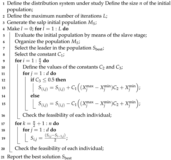
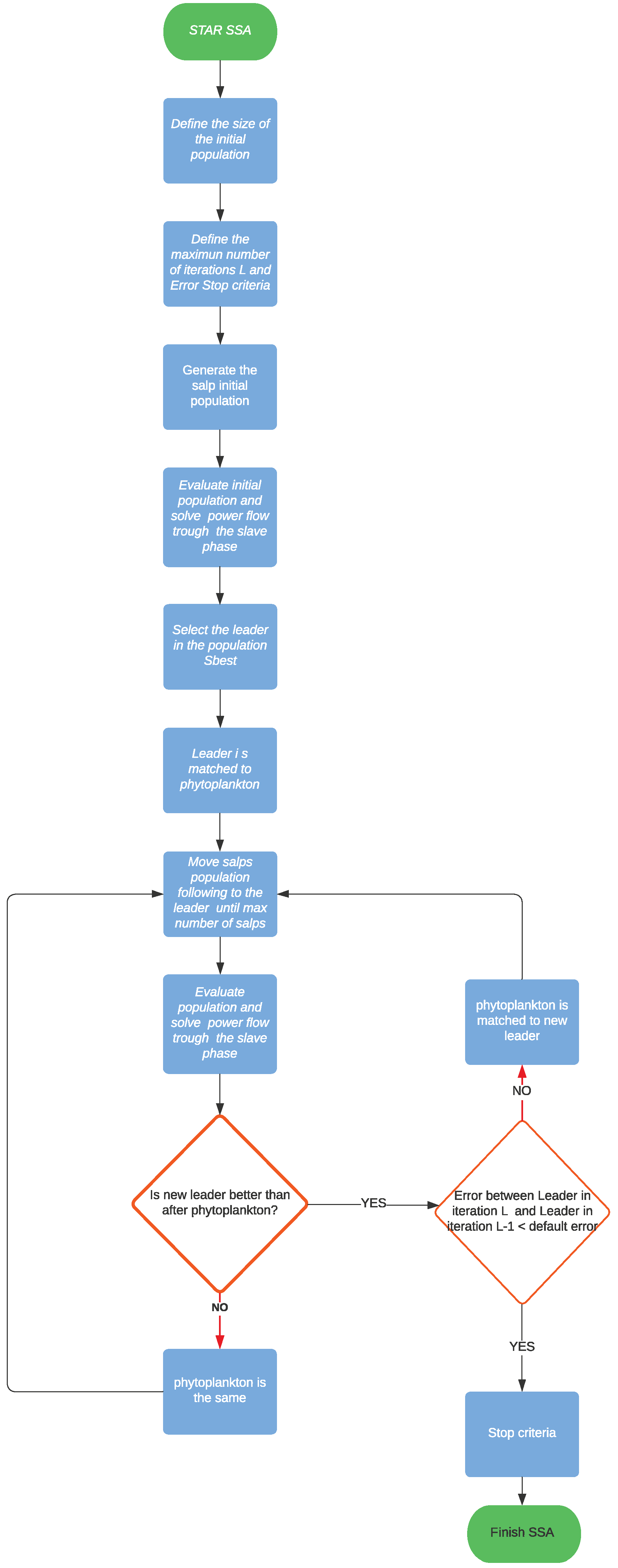
3.3. Summary of the Proposed Solution Methodology

With the purpose of illustrating the application of the SSA to general optimization problems, the Algorithm 1 is employed.
Algorithm 1: General application of the salp swarm algorithm to optimization problems.
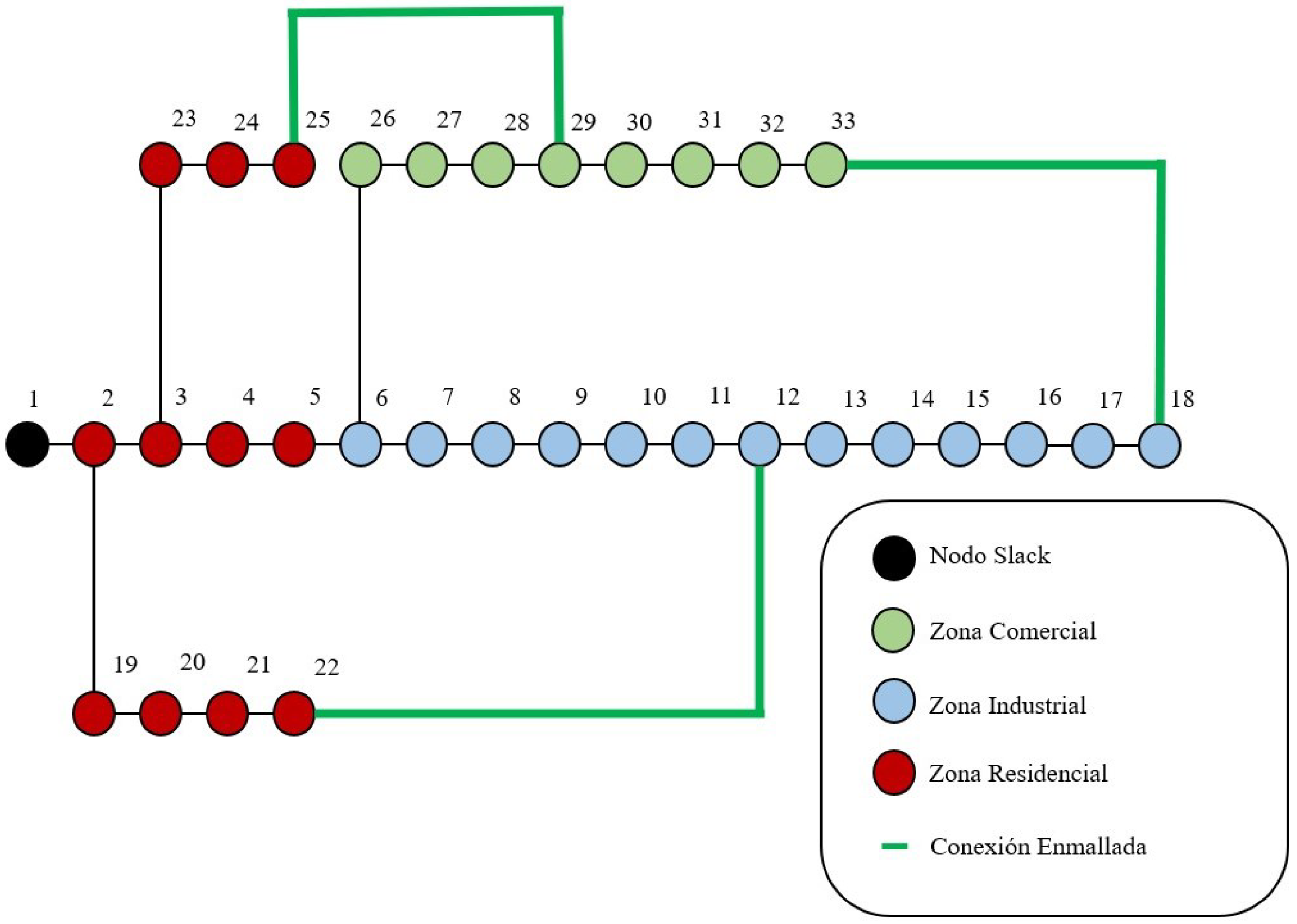
Algorithms 15 00345 i001
Additionally, in order to clarify the application of the SSA approach to locate and size D-STATCOMs in radial and meshed distribution networks, the flow chart of the proposed methodology is presented in Figure 1.

4. Test System

To evaluate the effectiveness of the proposed solution methodology for placing and sizing D-STATCOMs in medium-voltage distribution systems, the IEEE 33-node system is employed. The electrical configuration of this system is presented in Figure 2.
As for the parametric information of the network, the peak consumption data at each demand node are presented in Table 2.
Since this project is focused on selecting reactive compensators for radial and meshed distribution systems with varying demand according to the type of consumers across the distribution network, in order to evaluate these operating conditions, the demand data are considered according to that reported in [10], as shown in Table 3.
Note that the selection of these power consumption profiles was based on the typical load variation in a distribution circuit in the metropolitan area of Bogotá, Colombia. These values were estimated after multiple measurements taken during work days in a distribution substation operated with 11.4 kV. No geographical information is provided due to confidentiality commitments made with the energy distribution company.

5. Results and Discussion

To validate the proposed solution methodology, the solution of the optimization model for placing and sizing D-STATCOM in electrical distribution systems by using the AESDC was implemented in MATLAB’s R2021b version on a computer with an Intel Core i7-10750H @2.6 GHz and 16.0 GB of DDR4 RAM at 2300 MHz running the 64-bits version of Microsoft Windows 10 Home.

5.1. Radial Configuration Results

To verify the efficiency of the proposed solution methodology, 20 evaluations were performed for the radial configuration. The best result obtained had a cost of 108,249.36. Furthermore, this solution had a repeatability higher than 50% of the total evaluations. The best solution found for this test system corresponds to nodes 13, 25, and 30, with D-STATCOMs sizes of 258.51, 105.47, and 538.02 kvar, respectively. Note that, in this simulation, 20 individuals and 1000 iterations were set to evaluate the performance of the SSA.
The best five solutions reached by the methodology proposed for the IEEE 33-node system with a radial topology are presented in Table 4. The criteria used to select the five best solutions is the lowest operating cost using SSA without considering the execution time.
Note that the fifth result in Table 4 corresponds to a value of 108,428.91 dollars per year and defines the D-STATCOM locations at nodes 14, 10, and 30, with sizes of 180.37, 82.17, and 605.97 kvar, respectively. In this way, it can be stated that, for both the best and the worst solution, there is an optimal location at node 30. Furthermore, the difference between the two is 179.55 dollars, which means an approximate error of 0.166%. Even though this is a low error, it can be said that the gap between the two demonstrates that the solution space is large, despite the fact that they converge to a similar result.
The processing times for each algorithm evaluation regarding the best and worst result are 2.4317 and 2.0876 min, respectively. Which is an adequate computational effort due to the complexity of the studied problem. It is also important to mention that the nodes at which the D-STATCOMs are optimally placed are numbers 30 (commercial), 25 (industrial), and 13 (industrial).

5.2. Meshed Configuration Results

As with the radial topology, a population of 20 individuals (salps) was used to test the developed algorithm, as well as 20 consecutive evaluations of the whole methodology, considering 1000 iterations per evaluation. Table 5 summarizes the best five solutions obtained for the meshed IEEE 33-node system.
In the Table above, it is highlighted that the best result among the iteration entails operating costs of 77,870.17 dollars per year with D-STATCOMs located at nodes 32, 30, and 14, with powers of 202.30, 394.40, and 146.20 kvar, respectively. Note that the optimal solution for this algorithm was found 25% of the times that the entire methodology was evaluated. Moreover, the worst result entails 77,896.67 dollars per year and positions 30, 14, and 32, with sizes of 505.60, 176.20, and 98.20 kvar, respectively (see solution no. 5 in Table 5). The difference between the best and worst result is 26.50 dollars. Note that this difference is very small in comparison with the objective function values, which demonstrates that the proposed methodology can find very high-quality solutions in each evaluation.
Note that the processing times for each algorithm evaluation regarding the best and worst result are 1.9360 and 1.9392 min, respectively, i.e., the algorithm has a tendency towards finding the space and solution of the problem in similar periods of time.
The next section only compares the proposed algorithm within the meshed configurations, given that, in the specialized literature, the use of industrial, commercial, and residential curves in the studied problem has not yet been presented for radial configurations.

5.3. Comparative Analysis: Meshed Configuration

For the particular case of the meshed network, the baseline case presented in [10] was employed, as well as the XPRESS, SBB, DICOPT, and LINDO optimization algorithms available in the General Algebraic Modeling System software. The percentage differences for the aforementioned algorithms, in comparison with the proposed solution methodology, are favorable by 11.57, 2.13, and 1.90%, respectively. Table 6 shows the figures associated with the percentages describing the differences between the implemented solutions.
Finally, it is important to mention that the number of salps in the population was set as 20 in the radial and meshed configuration cases because of the compromise between the total processing time and the quality of the optimal solutions reached. This number of individuals was reached after constructing a meshed grid with sizes of populations between 5 and 30, evaluating the total processing time and the variability of the final solution after 100 consecutive iterations per population size.

6. Conclusions and Future Works

This paper studied the problem regarding the optimal placement and sizing of D-STATCOMs for electrical distribution networks with radial and meshed configurations. The optimization problem was formulated using an MINLP model, where the binary variables were associated with the nodes where the D-STATCOMs must be placed. The continuous variables were related to the power flow solution, i.e., the voltages, currents, and power variables. The objective of the MINLP model was to reduce the expected annual energy loss costs after installing D-STATCOMs across the distribution network. The main contribution of this research is the consideration of three different load profiles to classify the distribution grid as a function of energy usage (residential, industrial, and commercial). To solve the MINLP model, a master–slave optimization strategy was proposed. The master stage was entrusted with defining the nodes where the D-STATCOMs will be located and their corresponding sizes. In the slave stage, an efficient power flow formulation was implemented, which allowed calculating the expected annual grid operating costs. Numerical results in the IEEE 33-bus grid with radial and meshed configurations confirmed the effectiveness of the proposed solution methodology in comparison with the MINLP solvers available in the GAMS software.
An important result when comparing radial and meshed distribution topologies is that, even if the proposed optimization methodology is independent of the grid configuration, the expected annual operating costs are drastically affected by the grid configuration. The final objective function value was about USD/year 108,249.36, whereas, for the meshed topology, it was about USD/year 77,870.17, i.e., a difference of 30,379.19 dollars per year of operation. These differences are clearly explained by the nature of the meshed topology, where the voltage profiles are improved and a better distribution of the load flows is presented.
The main limitations of the proposed master–slave optimization method are its dependence on the experience of the programmer with the whole algorithm, including the selection of the algorithm parameters, in addition the fact that a statistical analysis is required to determine the average performance of the methodology regarding the objective function values and the processing times. Another important limitation of our proposal corresponds to its extension to power systems: even if the SSA approach can define the location and size of the reactive power compensators, the power flow employed in this research is only applicable to distribution networks without voltage-controlled nodes, which is not the case of power systems, where multiple power generates control voltage profiles in different nodes of the network. This implies the need for replacing the power flow solver with one that can deal with multiple voltage-controlled sources.
As future work, it will be possible to conduct the following studies: (i) combining D-STATCOMS and renewable energy resources to reduce the expected grid operating cost for a planning horizon of 10 or 20 years; (ii) considering the combination of D-STATCOMs and batteries in the same MINLP model and the proposed master–slave optimization methodologies using recently developed metaheuristic optimizers such as the generalized normal distribution optimizer and the arithmetic optimization algorithm; (iii) improving the mathematical formulation used to represent the D-STATCOMs in order to allow for simultaneous dynamic and steady-state analyses of the distribution network; and (iv) implementing new metaheuristic optimizers such as the Farmland Fertility algorithm, the African Vultures Optimization algorithm, and the Artificial Gorilla Troops algorithm to deal with the problem studied in this research.

Author Contributions

Conceptualization, methodology, software, and writing (review and editing): J.A.M.-B., C.D.F.-D. and O.D.M. All authors have read and agreed to the published version of the manuscript.

Funding

This research received no external funding.

Institutional Review Board Statement

Not applicable.

Informed Consent Statement

Not applicable.

Data Availability Statement

Not applicable.

Acknowledgments

This work derives from the undergraduate project Ubicación y dimensionamiento óptimo de D-STATCOMs en redes de distribución radiales empleando una versión discreta-continua del algoritmo de enjambre de salpas, presented by the students Cristian David Fonseca Díaz and Javier Andrés Mora Burbano to the Electrical Engineering Program of the Engineering Faculty at Universidad Distrital Francisco José de Caldas as a partial requirement for obtaining a Bachelor’s degree in Electrical Engineering.

Conflicts of Interest

The authors declare no conflict of interest.

References

  1. Sadovskaia, K.; Bogdanov, D.; Honkapuro, S.; Breyer, C. Power transmission and distribution losses—A model based on available empirical data and future trends for all countries globally. Int. J. Electr. Power Energy Syst. 2019, 107, 98–109. [Google Scholar] [CrossRef]
  2. Shaw, R.; Attree, M.; Jackson, T. Developing electricity distribution networks and their regulation to support sustainable energy. Energy Policy 2010, 38, 5927–5937. [Google Scholar] [CrossRef]
  3. Verma, H.K.; Singh, P. Optimal Reconfiguration of Distribution Network Using Modified Culture Algorithm. J. Inst. Eng. (India) Ser. B 2018, 99, 613–622. [Google Scholar] [CrossRef]
  4. Sultana, S.; Roy, P.K. Optimal capacitor placement in radial distribution systems using teaching learning based optimization. Int. J. Electr. Power Energy Syst. 2014, 54, 387–398. [Google Scholar] [CrossRef]
  5. Montoya, O.D.; Garces, A.; Gil-González, W. Minimization of the distribution operating costs with D-STATCOMS: A mixed-integer conic model. Electr. Power Syst. Res. 2022, 212, 108346. [Google Scholar] [CrossRef]
  6. Martin, O.; Terry, S.; Bottrell, N. Application of a Distribution STATCOM to Manage Network Voltages. In Proceedings of the 17th International Conference on AC and DC Power Transmission (ACDC 2021), Glasgow, UK, 7–8 December 2021. [Google Scholar] [CrossRef]
  7. Sirjani, R.; Jordehi, A.R. Optimal placement and sizing of distribution static compensator (D-STATCOM) in electric distribution networks: A review. Renew. Sustain. Energy Rev. 2017, 77, 688–694. [Google Scholar] [CrossRef]
  8. Marjani, S.R.; Talavat, V.; Galvani, S. Optimal allocation of D-STATCOM and reconfiguration in radial distribution network using MOPSO algorithm in TOPSIS framework. Int. Trans. Electr. Energy Syst. 2018, 29, e2723. [Google Scholar] [CrossRef]
  9. Montoya, O.D.; Chamorro, H.R.; Alvarado-Barrios, L.; Gil-González, W.; Orozco-Henao, C. Genetic-Convex Model for Dynamic Reactive Power Compensation in Distribution Networks Using D-STATCOMs. Appl. Sci. 2021, 11, 3353. [Google Scholar] [CrossRef]
  10. Castiblanco-Pérez, C.M.; Toro-Rodríguez, D.E.; Montoya, O.D.; Giral-Ramírez, D.A. Optimal Placement and Sizing of D-STATCOM in Radial and Meshed Distribution Networks Using a Discrete-Continuous Version of the Genetic Algorithm. Electronics 2021, 10, 1452. [Google Scholar] [CrossRef]
  11. Gomez-Gonzalez, M.; López, A.; Jurado, F. Optimization of distributed generation systems using a new discrete PSO and OPF. Electr. Power Syst. Res. 2012, 84, 174–180. [Google Scholar] [CrossRef]
  12. Salkuti, S.R. Optimal Allocation of DG and D-STATCOM in a Distribution System using Evolutionary based Bat Algorithm. Int. J. Adv. Comput. Sci. Appl. 2021, 12, 360–365. [Google Scholar] [CrossRef]
  13. Taylor, J.A.; Hover, F.S. Convex Models of Distribution System Reconfiguration. IEEE Trans. Power Syst. 2012, 27, 1407–1413. [Google Scholar] [CrossRef]
  14. Tanti, D.; Verma, M.; Singh, B.; Mehrotra, O. Optimal Placement of Custom Power Devices in Power System Network to Mitigate Voltage Sag under Faults. Int. J. Power Electron. Drive Syst. 2012, 2, 267–276. [Google Scholar] [CrossRef]
  15. Taher, S.A.; Afsari, S.A. Optimal location and sizing of DSTATCOM in distribution systems by immune algorithm. Int. J. Electr. Power Energy Syst. 2014, 60, 34–44. [Google Scholar] [CrossRef]
  16. Devi, S.; Geethanjali, M. Optimal location and sizing of Distribution Static Synchronous Series Compensator using Particle Swarm Optimization. Int. J. Electr. Power Energy Syst. 2014, 62, 646–653. [Google Scholar] [CrossRef]
  17. Gupta, A.R.; Kumar, A. Optimal placement of D-STATCOM in distribution network using new sensitivity index with probabilistic load models. In Proceedings of the 2015 2nd International Conference on Recent Advances in Engineering & Computational Sciences (RAECS), Chandigarh, India, 21–22 December 2015. [Google Scholar] [CrossRef]
  18. Faris, H.; Mirjalili, S.; Aljarah, I.; Mafarja, M.; Heidari, A.A. Salp Swarm Algorithm: Theory, Literature Review, and Application in Extreme Learning Machines. In Nature-Inspired Optimizers; Springer International Publishing: Berlin/Heidelberg, Germany, 2019; pp. 185–199. [Google Scholar] [CrossRef]
  19. Yuan, Z.; Paolone, M. Properties of convex optimal power flow model based on power loss relaxation. Electr. Power Syst. Res. 2020, 186, 106414. [Google Scholar] [CrossRef]
  20. Sharma, A.K.; Saxena, A.; Tiwari, R. Optimal Placement of SVC Incorporating Installation Cost. Int. J. Hybrid Inf. Technol. 2016, 9, 289–302. [Google Scholar] [CrossRef]
  21. Turgut, M.S.; Turgut, O.E.; Afan, H.A.; El-Shafie, A. A novel Master–Slave optimization algorithm for generating an optimal release policy in case of reservoir operation. J. Hydrol. 2019, 577, 123959. [Google Scholar] [CrossRef]
  22. Jaddi, N.S.; Abdullah, S. A cooperative-competitive master–slave global-best harmony search for ANN optimization and water-quality prediction. Appl. Soft Comput. 2017, 51, 209–224. [Google Scholar] [CrossRef]
  23. Suchite-Remolino, A.; Ruiz-Paredes, H.F.; Torres-García, V. A New Approach for PV Nodes Using an Efficient Backward/Forward Sweep Power Flow Technique. IEEE Lat. Am. Trans. 2020, 18, 992–999. [Google Scholar] [CrossRef]
  24. Shen, T.; Li, Y.; Xiang, J. A Graph-Based Power Flow Method for Balanced Distribution Systems. Energies 2018, 11, 511. [Google Scholar] [CrossRef]
  25. Garces, A. A Linear Three-Phase Load Flow for Power Distribution Systems. IEEE Trans. Power Syst. 2016, 31, 827–828. [Google Scholar] [CrossRef]
  26. Hegazy, A.E.; Makhlouf, M.; El-Tawel, G.S. Improved salp swarm algorithm for feature selection. J. King Saud Univ.-Comput. Inf. Sci. 2020, 32, 335–344. [Google Scholar] [CrossRef]
  27. Mirjalili, S.; Gandomi, A.H.; Mirjalili, S.Z.; Saremi, S.; Faris, H.; Mirjalili, S.M. Salp Swarm Algorithm: A bio-inspired optimizer for engineering design problems. Adv. Eng. Softw. 2017, 114, 163–191. [Google Scholar] [CrossRef]
  28. Gupta, A.R.; Kumar, A. Energy Savings Using D-STATCOM Placement in Radial Distribution System. Procedia Comput. Sci. 2015, 70, 558–564. [Google Scholar] [CrossRef]
  29. Montano, J.; Tobón-Mejia, A.F.; Rosales-Muñoz, A.A.; Andrade, F.; Garzón-Rivera, O.D.; Mena-Palomeque, J. Salp Swarm Optimization Algorithm for Estimating the Parameters of Photovoltaic Panels Based on the Three-Diode Model. Electronics 2021, 10, 3123. [Google Scholar] [CrossRef]
  30. Gholizadeh, S.; Danesh, M.; Gheyratmand, C. A new Newton metaheuristic algorithm for discrete performance-based design optimization of steel moment frames. Comput. Struct. 2020, 234, 106250. [Google Scholar] [CrossRef]
Figure 1. Flow diagram of the proposed SSA applied to the optimal location and sizing D-STATCOMs in distribution networks (See Section 3.1).
Algorithms 15 00345 g001
Figure 2. Electrical configuration of the IEEE 33-node system.
Algorithms 15 00345 g002
Table 1. Summary of methodologies used in the literature for the placement and sizing of D-STATCOMs.
Solution MethodologyObjective FunctionRef.Year
Artificial neural networksMitigation of voltage sags under faults[14]2012
Immune algorithmPower losses minimization and investment and operating costs reduction[15]2014
Particle swarm optimizationPower losses minimization and voltage profile improvement[16]2014
Sensitivity indexPower losses minimization and voltage profile improvement[17]2015
Discrete-continuous vortex search algorithmInvestment and operating costs reduction[9]2017
Multiobjective particle swarm optimizationPower losses minimization and voltage profile improvement[8]2019
Evolution-based bat algorithmPower losses minimization and voltage profile improvement[12]2021
Mixed-integer second-order cone programmingPower losses minimization and investment and operating costs reduction[5]2022
Table 2. Impedance and demand data for the IEEE 33-node system.
Node iNode j R ij ( Ω ) X ij ( Ω ) P j (kW) Q i (kvar)
120.09220.0477010060
230.49300.251109040
340.36600.1864012080
450.38110.194106030
560.81900.707006020
670.18720.61880200100
7817.114123.510200100
8910.3000.740006020
91010.4000.740006020
10110.19660.065004530
11120.37440.123806035
121314.680115.5006035
13140.54160.7129012080
14150.59100.526006010
15160.74630.545006020
161712.860172.1006020
17180.73200.574009040
2190.16400.156509040
19201.50421.355409040
20210.40950.478409040
21220.70890.937309040
3230.45120.308309050
23240.89800.70910420200
24250.89600.70110420200
6260.20300.103406025
26270.28420.144706025
272810.5900.933706020
28290.80420.7006012070
29300.50750.25850200600
30310.97440.9630015070
31320.31050.36190210100
32330.34100.530206040
Table 3. Load consumption profiles per user type: residential (Res.), industrial (Ind.), and commercial (Com.).
HourInd. (pu)Res. (pu)Com. (pu)
10.560.690.2
20.540.650.19
30.520.620.18
40.50.560.18
50.550.580.2
60.580.610.22
70.680.640.25
80.80.760.4
90.90.90.65
100.980.950.86
1110.980.9
120.9410.92
130.950.990.89
140.960.990.92
150.910.94
160.830.960.96
170.780.961
180.720.940.88
190.710.930.76
200.70.920.73
210.690.910.65
220.670.880.5
230.650.840.28
240.60.720.22
Table 4. Best five solutions found by the proposed solution methodology for the radial operation case.
Sol.NodesSizes (Mvar)Annual Costs
(USD/year)
Time
(min)
1 30 25 13 0.52801 0.10547 0.25851 108,249.362.3753
2 14 25 30 0.21204 0.11348 0.60418 108,368.922.1772
3 30 25 13 0.54889 0.13481 0.27254 108,371.632.3908
4 14 30 25 0.24129 0.60751 0.07779 108,422.552.1387
5 14 10 30 0.18037 0.08217 0.60597 108,428.912.4317
Table 5. Best five solutions found by the proposed solution methodology for the meshed operation case.
Sol.NodesSizes (Mvar)Annual Costs
(USD/year)
Time (min)
1 32 30 14 0.2023 0.3944 0.1462 77,870.171.9360
2 14 32 30 0.1394 0.2130 0.4002 77,872.481.9130
3 14 32 30 0.1902 0.1572 0.4327 77,890.141.9250
4 14 33 30 0.1011 0.1737 0.5155 77,894.511.9311
5 30 14 32 0.5056 0.1762 0.0982 77,896.671.9166
Table 6. Best results obtained for the baseline case; the XPRESS, SBB, DICOPT, and LINDO optimizers; and the proposed methodology.
CaseLocation (Nodes) and Sizing (Mvar)Cost (USD$/Year)
Baseline case86,882.81
XPRESS[13 (0.2000), 16 (0.0453), 32 (0.3923)]79,535.02
SBB, DICOPT, and LINDO[13 (0.0960), 16 (0.0531), 32 (0.4480)]79,350.36
Proposed algorithm[32 (0.2023), 30 (0.3944), 14 (0.1462)]77,870.17
Publisher’s Note: MDPI stays neutral with regard to jurisdictional claims in published maps and institutional affiliations.

