RSB: Robust Successive Binarization for Change Detection in Bitemporal Hyperspectral Images

Abstract

The Earth’s observation programs, through the acquisition of remotely sensed hyperspectral images, aim at detecting and monitoring any relevant surface change due to natural or anthropogenic causes. The proposed algorithm, given as input a pair of hyperspectral images, produces as output a binary image denoting in white the changed pixels and in black the unchanged ones. The presented procedure relies on the computation of specific dissimilarity measures and applies successive binarization techniques, which prove to be robust, with respect to the different scenarios produced by the chosen measure, and fully automatic. The numerical tests show superior behavior when other common binarization techniques are used, and very competitive results are achieved when other methodologies are applied on the same benchmarks.

1. Introduction

The task of change detection (CD) refers to those algorithms and methods that, given as input a collection of remotely sensed images, taken at different times of the same area, provide as output binary images where the white pixels denote the changed regions, while black pixels denote the unchanged parts; see [1] for a comprehensive survey. The CD task is especially useful in the Earth’s surface observation programs, which aim at monitoring any relevant change in the environment due, for example, to natural disasters [2,3], urban expansions, agricultural habits and so on; see [4] and references therein for a broad overview.

Hyperspectral (HS) sensors remotely acquire data observations at high spectral and spatial resolution. In particular, every HS image can be thought of as a three-mode tensor, where, in the first and second mode, the spatial information is stored, while, in the third mode, the spectral information is registered at specific, predetermined wavelengths of the light. Hence, for every pixel, a hundred regularly spaced narrow bands are stored, allowing for a great abundance of information. For this reason, a common denominator of many CD methods is the use either of matrix or tensor factorizations [5,6,7,8], or autoencoder architectures; see, e.g.,  [9,10], which can provide a reasonable representation in suitable subspaces of reduced dimensions, allowing one to eliminate redundancies while keeping the relevant features. Another strong motivation for using matrix or tensor decompositions is to remove the noise affecting the original HSI or to restore the missing information; see, e.g., [11,12,13,14] for recent advances regarding this topic. Taking care of the preprocessing phase has been proven to significantly improve the final CD results; see [15]. In this work, however, since most of the publicly available datasets for CD are already preprocessed, this step is not implemented.

A second common component in many CD algorithms is the use of specific similarity or dissimilarity functions (sometimes called error functions) that, hence, produce several types of scenarios. Most algorithms do not provide an automatic selection of the best output, but all of the produced outputs are analyzed and the optimal results are selected via post-analysis, i.e., after the evaluation, the best binary change map is the one with the higher computed accuracy. On the one hand, in certain cases, very accurate results can be achieved with a specific configuration—see, e.g., [16]—but on the other hand, such approaches are still limited in real applications when the reference binary change map, i.e., the ground-truth image, is not available to provide a post-analysis evaluation.

In this work, a new method is proposed that does not use any initial projection and that computes a suitable mean image given 6 types of error functions. This strategy is therefore robust with respect to the chosen function and it is automatic, i.e., the best choice is not obtained via any post-analysis.

After the similarity or dissimilarity phase, usually, a binarization technique is applied, either by using clustering [17,18] or via automatic thresholding techniques [19,20]. Here, a novel thresholding method is also proposed. In particular, three binarization procedures are formulated and applied successively. In the first one, for every error function, a collection of 5 different binary images are produced and a suitable mean image is computed. Then, this mean image is again binarized by setting to 0 any pixel value below 1 and setting to 1 any pixel value originally greater than 1. Lastly, the newly produced mean images for every error function are summed together and binarized again according to a new threshold value. This type of successive binarization is compared against the most commonly adopted thresholding techniques.

Finally, it is also important to recall that while, originally, many methods were formulated within an unsupervised framework, recently, many new approaches have been derived exploiting deep learning by constructing very innovative architectures and hence producing robust results; see, e.g., [21,22,23,24,25].

In summary, the presented method hinges on the following three steps:

• Successive binarization techniques are proposed by varying the thresholding value, which can be considered fixed every time, i.e., not adaptively varying and not a free parameter, if the proposed types of error functions are the ones adopted here.
• Among the used error functions, a new one based on the Pearson correlation coefficient is introduced.
• Robustness with respect to the error function is achieved by computing a suitable mean image: the produced output is a suitable weighted sum of every contribution.

The paper is organized as follows. In Section 2, the proposed algorithm is detailed. In Section 3 and Section 4, the numerical experiments are carried out. In Section 5, the obtained results are discussed and compared with other available techniques. In Section 6, some conclusive comments are given.

2. Methodology

Two HS images ${\mathcal{I}}_1$ and ${\mathcal{I}}_2$, acquired at two different time steps for the same area, are given. Denoting with $m\times n\times k$ the size of ${\mathcal{I}}_1$ and ${\mathcal{I}}_2$, each HS image is rearranged into a matrix $I_1$ and $I_2$, respectively, with size $p\times k$, with $p=mn$. The CD methodology in Algorithm 1 is proposed. The first step (line 2) consists in computing 6 error functions selected by previous and intensive experiments on several datasets; see [17,26,27]. More specifically, let the considered error function be denoted with $f_i$, having i ranging between 1 and 6. To be self-contained, the description of the chosen error functions is reported in the following Section 2.1.

2.1. Error Functions

Many error functions could be used to assess possible changes; however, here, the following ones have been selected.

• Euclidean distance ($i=1$): The difference between every spectral row vector in $I_1$ and $I_2$ is computed. Then, the second norm of the resulting difference vectors is calculated. The computational cost for this metric is proportional to $O\left(pk\right)$.
• Manhattan distance ($i=2$): The norm 1 is computed on the spectral difference vectors. The computational cost is proportional to $O\left(pk\right)$.
• SAM-ZID ($i=3$)—see [16]: Firstly, the sinus of the angle between every spectral row vector in $I_1$ and $I_2$ is computed and then scaled in $[0,1]$; secondly, the obtained result is multiplied by the standardized difference vector, again scaled in $[0,1]$. The computational cost is proportional to $O\left(2pk\right)$.
• Spatial Mean SAM—in short, SAM-MEAN ($i=4$): The arithmetic mean of the angles between two pairs of spectral vectors (i.e., one row vector in $I_1$ and another row vector in $I_2$) inside a local window is computed. The computational cost is $O(4pk+2d_V-1)$, where, by $d_v$, we denote the chosen window size; see [28] for the details about this parameter.
• Spatial Mean Spectral Angles Deviation Mapper—in short, SMSADM ($i=5$): The arithmetic mean of the deviation angles from their spectral mean is computed inside a local window, which slides through the considered image. The computational cost is $O(4pk+2d_V-1)$, where, again, by $d_v$, we denote the chosen window size.
• A complementary measure of the Pearson correlation coefficient, denoted in short as Pearson cc, ($i=6$): The Pearson correlation coefficient [29] is computed between every pair of spectral row vectors. This is not a common error function to measure changes, but it is experimentally proven to be insightful; see [30]. Here, we propose the following novel formulation. The Pearson coefficient, computed for every spectral row vector, is a value $\rho$ between $-1$ and 1. In particular, $\rho =-1$ means a negative linear correlation, while $\rho =1$ means a positive linear correlation. Values of $\rho$ near the 0 mean either very low or no correlation at all. In order to use $\rho$ as a suitable indicator for the change detection task, firstly, it is computed as $\left|\rho \right|$, to eliminate any negative numbers (which would be meaningless in terms of pixel intensity values) and then it is mirrored with respect to one, so $1-\left|\rho \right|$. In fact, a high correlation is expected among the unchanged pixels, in the background, since the same area is analyzed at two different time steps, and hence, for those pixels, the corresponding $\left|\rho \right|$ should be close to 1. Meanwhile, regarding the changed pixels, it is unlikely to obtain any possible linear correlation, i.e., the $\rho$ values should be small or even 0. Therefore, to obtain a suitable output that highlights changes, the  $\left|\rho \right|$ produced for every spectral row vector is mirrored with respect to one, so that 0 or close to 0 values will become closer to 1 and the corresponding pixels will have higher intensity values. The computational cost is $O\left(6pk\right)$.

Algorithm 1: RSB pseudo-code

Data: Given $I_1,I_2$ HS vectorized images Result: Binary change map 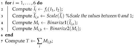output: $Binarize3\left(T\right)$;

The chosen error functions are selected by considering that both spatial and spectral changes should be detected. The error functions $f_1$ and $f_2$ account both for the spatial distribution; the error functions $f_3$, $f_4$ account for the spectral distribution; the error function $f_5$ is a hybrid measure and accounts for spectral and spatial distribution together, and, finally, the function $f_6$ highlights the areas that are highly not correlated and hence possibly changed.

Remark 1.

Note that the functions $f_4$ and $f_5$, i.e., SAM-MEAN and SMSADM, have been experimentally proven to remarkably improve the classical SAM [31] and SSCC [32], when HS images are analyzed; see [27] for additional details, and refer to [33] and references therein for other types of error functions.

2.2. The Algorithm

For the bi-temporal pair of HS images $(I_1,I_2)$, the generation of the final binary change map is carried out by using the following robust successive binarization (RSB) procedure:

• Application of an error function $f_i$, which gives as output an image denoted by ${\tilde{I}}_i$, for every $i=1,\dots ,6$, line 2 in Algorithm 1.
• Scaling in the range $[0,1]$ the intensity values of ${\tilde{I}}_i$, to obtain ${\tilde{I}}_{i,s}$, line 3 in Algorithm 1.
• Binarize ${\tilde{I}}_{i,s}$ by applying different threshold values, line 3 in Algorithms 1 and 2. In particular, let us denote with $\epsilon =0.2,0.3,0.4,0.5,0.6$ the chosen thresholds. The pixels in ${\tilde{I}}_{i,s}$ are screened against the values of $\epsilon$, producing 5 differently binarized images, for every analyzed ${\tilde{I}}_{i,s}$. Hence, selecting any ${\tilde{I}}_{i,s}$, the pixels greater than or equal to the value of the current $\epsilon$ are set to 1 (i.e., they will be white), and the others, less than $\epsilon$, will be set to 0, i.e., black pixels. We denote the resulting image with ${\tilde{I}}_{i,s,\epsilon }$, for the chosen value of $\epsilon$. The computational cost for this procedure is $O(5p+5)$. It should be noted that this process is commonly performed by an automatic thresholding technique, such as Otsu’s thresholding method; see [34]. The choice to produce 5 different outputs though is preferable here, as we are not seeking to produce the best binarized possible image, for which an adapting thresholding technique should be employed. The goal here is to produce a set of different possible binary images, which is achieved more easily in the following.
• A suitable mean image is then computed as

  $$M_i=\frac{{\displaystyle \sum _{\epsilon }{\tilde{I}}_{i,s,\epsilon }}}{2}.$$
  The choice to divide by 2 rather than by 5, as it would be in the common mean definition, is motivated by the fact that we are looking to sum together the contributions of the two sought classes of changed and unchanged pixels. Since it is not a priori known which of the 5 produced binary images are the best ones to make the two classes fairly separable, all ${\tilde{I}}_{i,s,\epsilon }$ are considered, but it is assumed that the contribution provided by these 5 images, under a theoretical point of view, should sum up to 2.
• Every image $M_i$, for $i=1,\dots ,6$, is then itself binarized (line 5 in Algorithms 1 and 3) by setting to 1, i.e., white, the pixels whose intensity is greater than or equal to 1, and setting to 0, i.e., black, the pixels with intensity values less than 1. The computational cost for this procedure is $O\left(p\right)$. This step, for every fixed i, will produce an image denoted with $M_{i,b}$ whose entries are only integer values of 0 s and 1 s.
• The next step consists in computing the following image:

  $$\begin{array}{c}\hfill T=\sum _{i=1}^6{M}_{i,b}.\end{array}$$
• Since T is obtained by summing integer quantities, when the white pixels are present on the same areas, the resulting entries in T will be equal to 6; on the contrary, if only black pixels are present in a certain spot, the corresponding entries in T will be 0. An interesting case arises when, on the same regions, in some cases, there are white pixels, and in other cases, there are black ones. In particular, T is binarized according to the following rule:
  • Pixels with an intensity value greater than or equal to 3 are set to 1 and hence will be white, i.e., changed ones;
  • Pixels with values less than 3 are set to 0, and hence they will denote unchanged areas.
  This procedure is summarized in Algorithm 4 and it costs $O\left(p\right)$.
  The adopted error functions are dissimilarity measures; hence, the higher values are provided when different areas, either in the spatial domain or in the spectral domain, are analyzed. However, it can happen that, due to different light conditions, similar areas could be perceived as different ones, and hence, as a result, the corresponding pixels could receive a high intensity value in the computed ${\tilde{I}}_i$ image. This possible scenario does not necessarily appear in every ${\tilde{I}}_i$ for every used error function $f_i$; thus, the best value to threshold the computed output is set to 3 for the following reason. There are two error functions to detect changes in the spatial domain (i.e., $f_1,f_2$) and in the spectral domain (i.e., $f_3,f_4$); then, there is a hybrid error function for the spectral–spatial domain ($f_5$) and another function for detecting any linear correlation in the background ($f_6$). The functions $f_1$ and $f_2$ on the one side, and the functions $f_3$ and $f_4$ on the other, behave pair-wise similarly. Therefore, any analyzed pixel cannot be wrongly classified more than twice, since $f_5$ is a hybrid function that should smooth out any contradictory behaviors of the previous functions and $f_6$ measures a different indicator.

Algorithm 2: Binarize1 pseudo-code

Data: Given a matrix A Result: Binary mask 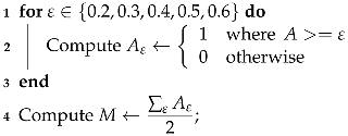output: M;

Algorithm 3: Binarize2 pseudo-code

Data: Given a matrix M Result: Binary mask 1 Compute $M_b\leftarrow \left\{\begin{array}{cc}1& \mathrm{where}M>=1\hfill \\ 0& \mathrm{otherwise}\hfill \end{array}\right.$; output: $M_b$;

Algorithm 4: Binarize3 pseudo-code

Data: Given a matrix T Result: Binary mask 1 Compute $T_b\leftarrow \left\{\begin{array}{cc}1& \mathrm{where}T>=3\hfill \\ 0& \mathrm{otherwise}\hfill \end{array}\right.$; output: $T_b$

3. Numerical Experiments

The numerical experiments are performed with an Intel Core I7-6500U 2.50 GHz, 8 GB RAM, and the following benchmark datasets are analyzed:

• Hermiston dataset (The dataset can be downloaded at: https://gitlab.citius.usc.es/hiperespectral/ChangeDetectionDataset/-/tree/master/Hermiston access date 15 August 2022) consists of two coregistered HS images over the city of Hermiston, Oregon, in 2004 and in 2007. The images are acquired by the Hyperion sensor and consist of $390\times 200$ pixels with 242 spectral bands; see Figure 1 for the RGB rendering of this dataset.
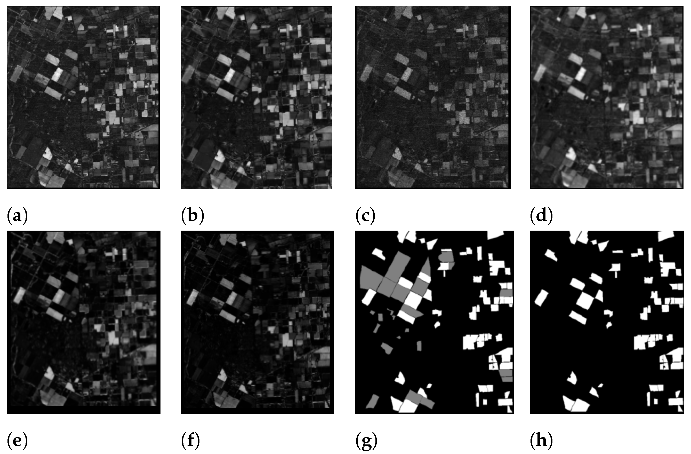
• USA dataset (The dataset can be downloaded at: https://rslab.ut.ac.ir/documents/81960329/82034892/Hyperspectral_Change_Datasets.zip access date 15 August 2022) consists again of two HS images acquired by the Hyperion sensor over Hermiston in Umatilla County, on 1 May 2004, and 8 May 2007, respectively. The land cover types are soil, irrigated fields, river, building, types of cultivated land, and grassland. These two HS images consist of $307\times 241$ pixels and 154 spectral bands; see Figure 2 for the RGB rendering of this dataset.
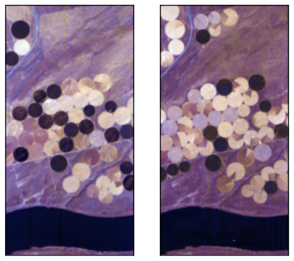
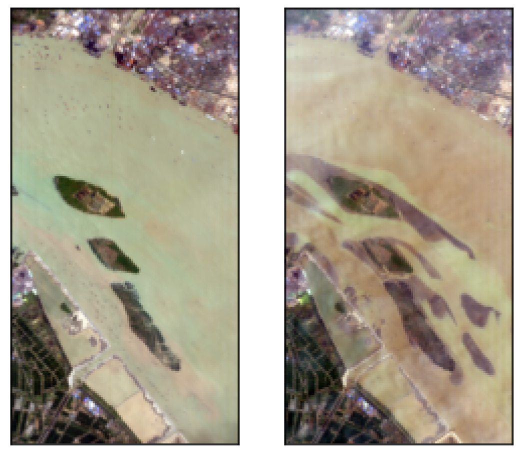
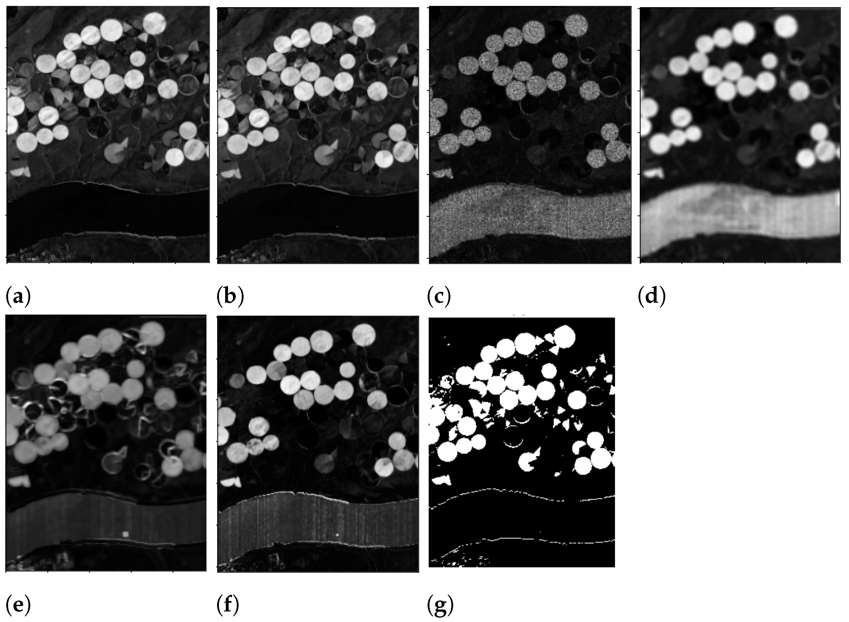
• River (The dataset can be downloaded at: http://crabwq.github.io access date 15 August 2022) dataset [35] contains two HS images taken in Jiangsu Province, China, acquired on 3 May 2013 and on 31 December 2013, respectively, by the (EO-1) Hyperion sensor; see Figure 3 for the RGB rendering of this dataset. These two images consist of $463\times 241$ pixels with only 198 spectral bands after noise removal.
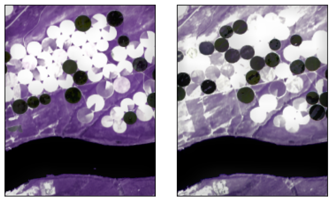
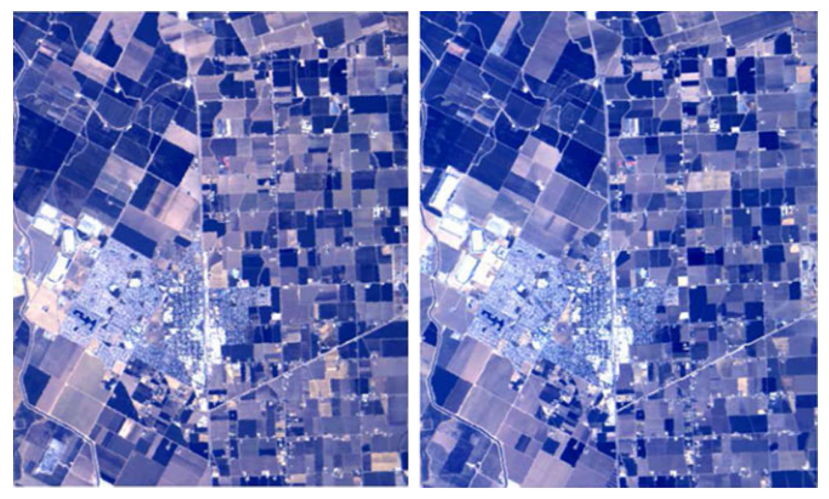
• Bay Area (The dataset can be downloaded at https://gitlab.citius.usc.es/hiperespectral/ChangeDetectionDataset/-/tree/master/bayArea access date 15 August 2022) dataset consists of two HS images taken in the years 2013 and 2015 with the AVIRIS sensor surrounding the city of Patterson (California). The spatial dimension is $600\times 500$ pixels and there are 224 spectral bands. In the available ground truth, $75.79\%$ of the total number of pixels are not classified, i.e., do not have any label. These images were coregistered by using the HypeRvieW desktop tool; see [36,37] and Figure 4 for the RGB rendering.

The choice of these datasets is not casual as they can be considered typical benchmarks to assess the accuracy of the CD algorithm for three different cases. Indeed, in the Hermiston ground truth, in Figure 5g and, the changed areas have a very clear and neat silhouette; in the USA dataset ground truth, in Figure 6g, the changed areas have both neat profiles as well as fragmented and very thin boundaries. Finally, in the ground truth of the River dataset, in Figure 7g, the majority of the changed areas look very fragmented and no clear shapes can be highlighted. Regarding the Bay Area ground-truth, Figure 8h, the same observation as in the Hermiston case hold. The goal of change detection algorithms is to provide a method that would achieve good accuracy regardless of the shape of the changed areas; hence, it is important to test the proposed methodology at least on these three different types of scenarios. In all four cases, the RBG rendering, produced by applying the algorithm in [38], is performed only for visualization purposes.

3.1. Preliminary Discussion

In Figure 5, Figure 6, Figure 7 and Figure 8, the image ${\tilde{I}}_i$ is shown, for $i=1,\dots ,6$, for all the considered datasets, by varying the adopted error function $f_i$ with $i=1,\dots ,6$. After this first step, for the Hermiston dataset, it is clear that $f_1$ and $f_2$ are producing some relevant noise around the changed areas, while $f_3$ and $f_4$ produce a better output but also the river silhouette appears at the bottom of the images. Regarding $f_5$ and $f_6$, these two functions produce the best output. Although there are pixels that could be wrongly classified if $f_1$, $f_2$, $f_3$, and $f_4$ were considered separately; after step 7 of the proposed algorithm in Section 2, the wrong detections would be completely discarded.

Regarding the USA dataset, the functions that produce the best output, according to the given ground truth, are $f_1$ and $f_2$. All the others fully highlight the river at the bottom of the image. In particular, the worse output is given by $f_3$ and $f_4$, while the function $f_5$ produces a less visible river shape and some interesting details in the upper part of the image, and the function $f_6$ yields a too clean output in the upper part of the image and a still visible river shape at the bottom of it.

Regarding the River dataset, all the assayed functions produce a reasonable output. Only $f_6$ gives a very dark image as the $\rho$ values for the considered spectral row vectors are found to be very small.

Finally, in the Bay Area dataset, after suitably scaling each spectral vector of $I_2$ within the same range of values of the corresponding spectral vectors in $I_1$, for the error functions $f_i,i=1,\dots ,4$, a gamma correction with $\gamma =0.2$ to enhance brightness was necessary to improve the frequency ranges.

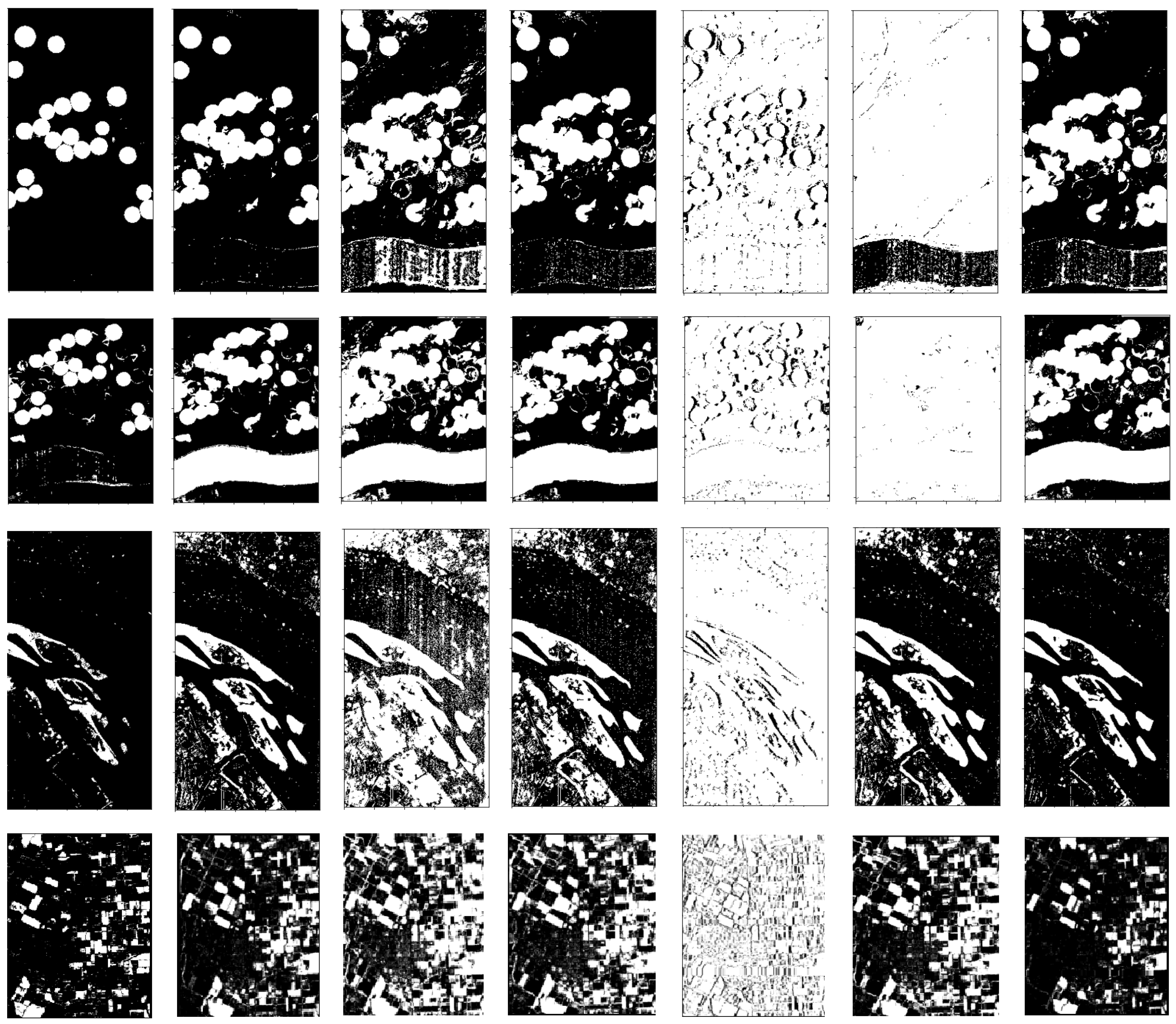
3.2. Thresholding Robustness

In order to show the robustness of proposed successive binarization technique with respect to the chosen error functions, in Figure 9, the output obtained with the proposed algorithm RSB (first column) is shown together with that of other thresholding methods. In particular, the output of the following methods is shown: in the second column, Otsu’s thresholding; in the third column, the mean thresholding [39]; in the fourth column, the Li thresholding [40]; in the fifth column, the Sauvola thresholding [41]; in the sixth, the triangle thresholding [42], and, finally, in the last column, the Yen thresholding [43].

It is also worth mentioning that the minimal thresholding technique [39,44] could not be successfully applied due to the absence of two maxima in the intensity value histograms and the fact that the local thresholding technique [45] provided as output completely black images, regardless of the size of the chosen local sliding window.

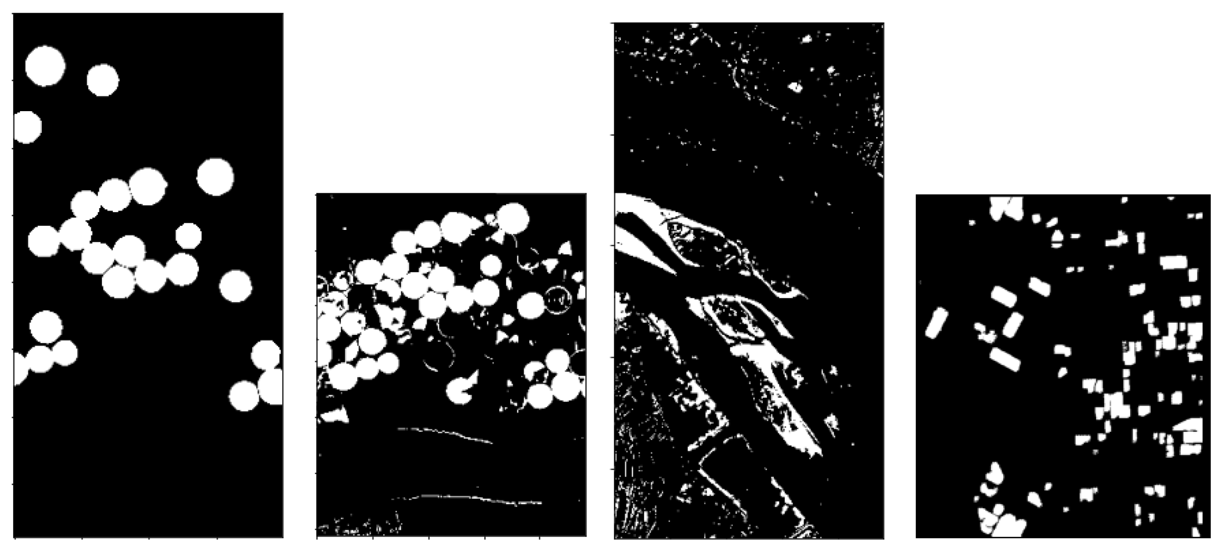
3.3. Results Evaluation

To assess the quality and the accuracy of the final produced results, two common indicators are adopted: the overall accuracy (OA) and the Kappa coefficient (K). In particular, OA expresses the fraction of the correctly classified pixels with respect to the total number of pixels,

$$\begin{array}{c}\hfill \mathrm{OA}:=\frac{(\mathrm{TP}+\mathrm{TN})}{(\mathrm{TP}+\mathrm{FP}+\mathrm{FN}+\mathrm{TN})}.\end{array}$$

The OA indicator sometimes appears to be biased; for example, in the case of a completely black output, since the black pixels constitute the majority of the pixels in the ground truth, the computed OA could still be slightly greater than $0.50$, which is obviously a faulty accuracy evaluation. Hence, to obtain a more reliable result, the Kappa coefficient is also computed as

$$\begin{array}{ll}\mathrm{K}& :=\frac{\mathrm{OA}-p}{1-p},\\ p& :=\frac{(\mathrm{TP}+\mathrm{FP})(\mathrm{TP}+\mathrm{FN})}{{(\mathrm{TP}+\mathrm{TN}+\mathrm{FP}+\mathrm{FN}) }^2}+\frac{(\mathrm{FN}+\mathrm{TN})(\mathrm{FP}+\mathrm{TN})}{{(\mathrm{TP}+\mathrm{TN}+\mathrm{FP}+\mathrm{FN}) }^2}.\end{array}$$

In both the above expressions, the used symbols correspond to

-

TP: true positive,

-

TN: true negative,

-

FP: false positive,

-

FN: false negative.

Note that the ideal classifier would give OA and K equal to 1. Hence, the aim of CD algorithms is to produce binary change maps that should have both OA and K as close as possible to 1. In

Table 1. Comparisons with other thresholding techniques. RSB achieves the best results (in bold).

Thresholding	Hermiston		USA		River		Bay Area
	OA	K	OA	K	OA	K	OA	K
RSB	0.9867	0.9410	0.9076	0.7060	0.9624	0.7250	0.8935	0.5873
Otsu	0.9633	0.8522	0.7323	0.3939	0.9061	0.5970	0.8335	0.5134
Mean	0.7691	0.4155	0.6939	0.3960	0.5637	0.1595	0.6585	0.2882
Li	0.9028	0.6710	0.7276	0.4225	0.8091	0.3946	0.7190	0.3525
Sauvola	0.2029	0.0223	0.2822	0.0302	0.1403	0.0104	0.2833	0.0483
Triangle	0.2543	0.0415	0.2330	0.0043	0.8474	0.4628	0.7427	0.3820
Yen	0.8579	0.5663	0.7117	0.4079	0.9409	0.6977	0.8865	0.5962

, we report the results obtained by varying the thresholding method. The algorithm proposed here, RSB, provided the higher OA and K for all three assayed datasets. The Otsu thresholding method gave the second best output for all the considered datasets, while the worst results where achieved when using the Sauvola and triangle thresholding methods.

4. Post-Processing

In order to improve the achieved results with RSB, some post-processing (PP) techniques could be applied. Since this step comes after a post-analysis of the obtained output, a suitable technique can be chosen on the basis of the obtained binary change map.

4.1. Morphological Transformations

Regarding both the Hermiston and the Bay Area dataset, the white regions of the RSB-produced change map (Figure 9, the first picture in the first row and the first picture in the last row) appear very neat and with a precise silhouette; therefore, it is appropriate to use a noise removal filter, in order to eliminate the spurious noisy pixels. To this end, a morphological opening transformation (see, e.g., [46], Chapter 5) with the following kernel is applied:

$$\begin{array}{c}\hfill Kernel=\left(\begin{array}{ccccc}0& 0& 1& 0& 0\\ 0& 1& 1& 1& 0\\ 1& 1& 1& 1& 1\\ 0& 1& 1& 1& 0\\ 0& 0& 1& 0& 0\end{array}\right).\end{array}$$

The obtained results for the Hermiston and the Bay Area datasets are discussed in Section 5 and the produced final binary change maps are shown in Figure 10, in the leftmost sub-figure and in Figure 10, in the rightmost sub-figure, respectively.

4.2. Supervised Classifier

Regarding the other two datasets, USA and River, the produced change maps (Figure 9, first pictures in the second row and in the third row, respectively) look very detailed and, hence, it is not advisable to use a pixel-wise noise removal filter, as important information could be lost. Therefore, the obtained binary change maps are used as pseudo-labels to train a supervised classifier. Note that this step is now performed without using the exact ground truth. In particular, a Gaussian Naive Bayes algorithm is applied. Naive Bayes methods are a set of supervised learning algorithms based on applying Bayes theorem with the “naive” assumption of conditional independence between every pair of features, given the value of the class variable. Therefore, every feature distribution can be individually estimated: this implies an ability to solve many mono-dimensional problems, which in turn can alleviate the computational cost when large matrices or tensors are processed. Moreover, besides being rather efficient, Naive Bayes are considered optimal in many applications [47]. In our specific case, the likelihood of every feature is assumed to be modeled by a Gaussian distribution, where the unknown mean and standard deviation, for every Gaussian, are estimated via the maximum likelihood algorithm. The Gaussian Naive Bayes (GNB) is run twice. The first time, for the training and test set, the difference image $|I_1-I_2|$ for the USA and River dataset is constructed and the output of the RSB change maps are used as “exact” labels. The second time, the ”exact” labels are replaced by the output produced by the first iteration. The implementation is done by using scikit-learn [48], and on the first iteration, the algorithm is run with the default parameters, while on the second iteration, the parameter var_smoothing is set to $1.{125210}^{-3}$ for the USA dataset and to $1.0$ for the River dataset. The finetuning of such parameters is not a trivial task; although quite elaborate techniques exist, since this is outside the scope of the current paper, for our purpose, the chosen values have been experimentally found. The obtained results after this PP step are shown in

Table 2. Output of the Gaussian Naive Bayes.

Datasets	1 Iteration		2 Iterations
	OA	K	OA	K
USA	0.9535	0.8609	0.9579	0.8781
River	0.9609	0.7711	0.9681	0.8014

. Applying GNB, after the first iteration, remarkably improves both OA and K for the USA dataset, while, for the River dataset, the OA is slightly reduced, but K is largely increased. After the second iteration, for both datasets, the OA indicator is slightly increased, but K is highly improved, hence providing a more accurate output. The final produced change maps are shown in Figure 10, in the second and third picture for the USA and River dataset, respectively.

5. Discussion

In this section, we compare the obtained accuracy results with other methods available in the literature, whose results have been published.

For the Hermiston dataset, in

Table 3. The proposed approach, RSB, with post-processing, and other competitors on the Hermiston dataset. The best results are displayed in bold.

Method	Hermiston
	OA	K
RSB+PP	0.9876	0.9447
AI-QLP [50]	0.9856	0.9400
Method [10]	0.9874	−
BIC2 [17]	0.9881	−
ORCHESTRA [51]	0.9871	−
GETNET [18]	0.9540	0.7810
CVA [18]	0.9390	0.6610
PCA-CVA [18]	0.9790	0.9060
CNN [18]	0.9470	0.7600
CUDA [20]	0.9848	−
AICA [49]	0.9887	−
SFBS-FFGNET [18]	0.9850	0.9310

, the achieved results produced by other methods are reported. In particular, in the table, for each method, a reference in which the reported results are published is provided. The method AICA [49] achieves the best OA, but there is no automatic selection of the best output, while the method proposed here obtains the third best OA. Among the methods that provide also the K values, our method, RSB, yields the highest value. The considered competitors are the following: AI-QLP [50], an approximate iterative QLP decomposition; the method in [10], which also works for multi-class change detection classification; BIC2 [17], a methodology based on iterative clustering; ORCHESTRA [51], an autoecoder-based approach; GETNET [35], a method based on an end-to-end 2D convolution neural network; CVA [19], an approach that exploits change vector analysis; PCA-CVA [52], enhanced PCA, and inverse triangular function-based thresholding, which are used together with change vector analysis; CNN [23], an approach based on autoencoder, clustering, and pseudo-label generation; CUDA [20], a method that exploits similarity measures, PCA, and the automatic Otsu thresholding; and SFBS-FFGNET [18], a CNN framework with slow–fast band selection and feature fusion.

Regarding the USA dataset, the results are reported in

Table 4. The proposed approach, RSB, with post-processing, and other competitors on the USA dataset. The best results are displayed in bold.

Method	USA
	OA	K
RSB+PP	0.9579	0.8781
GETNET-1 [35]	0.9289	0.7764
GETNET-2 [35]	0.9332	0.7897
CVA [19]	0.9272	0.7670
MAD-SVM [56]	0.8612	0.4760
IR-MAD-SVM [56]	0.9285	0.7700
Method [56]	0.9490	0.8310
BIC2 [17]	0.9728	−
AICA [49]	0.9417	−
HybridSN [24]	0.9553	0.8701
SCNN-S [24]	0.9631	0.8848
SSCNN-S [24]	0.9651	0.8918
TRIFCD-MS [7]	0.8848	0.7024
TRIFCD-Fusion [7]	0.9263	0.7813
BCG-Net [58]	0.9546	0.8662

, and again, a reference is provided for the published results. Here, BIC2 [17] achieves the best OA, but again, there is no automatic selection of the best scenario, while the best value for K is provided by the method SSCNN-S [24], a spectral–spatial convolutional neural network approach realized with a Siamese architecture. Among all the proposed approaches, the method here presented, RSB, achieves good accuracy (OA = 0.9579), which is behind only advanced methods based on iterative learning and ad hoc neural network architectures, and it also yields the third best K value (K = 0.8781). The analyzed competitors are GETNET-1 and GETNET-2, which denote an end-to-end 2D convolutional neural network without unmixing and with unmixing, respectively; CVA [19], MAD-SVM, and the multivariate alteration detection method (MAD [53]), where the thresholding operation is carried out via SVM; IR-MAD-SVM, the iteratively reweighted MAD [54,55], where, again, the thresholding selection is done via SVM; the method proposed in [56], which is based on 3D convolution deep learning; BIC2 [17]; AICA [49]; HybridSN [57], a hybrid spectral CNN; SCNN-S [24] and SSCNN-S [24], which denote a spectral convolutional NN with a Siamese architecture and a spectral–spatial convolutional NN with a Siamese architecture, respectively; TRIFCD-MS [7] and TRIFCD-Fusion [7], methods based on the simultaneous fusion of low-spatial-resolution HS images and low-spectral-resolution MS images with the use of a tensor regression; and BCG-Net [58], an architecture driven by a partial Siamese united unmixing module, together with multi-temporal spectral unmixing and a temporal correlation constraint.

For the River dataset, the RSB method achieves the best OA and K values compared to all the other methods considered, see

Table 5. The proposed approach, RSB, with post-processing, and other competitors on the River dataset. The best results are displayed in bold.

Method	River
	OA	K
RSB+PP	0.9681	0.8014
GETNET-1 [35]	0.9497	0.7662
GETNET-2 [35]	0.9514	0.7539
CVA [19]	0.9529	0.7967
PCA-CVA [52]	0.9434	0.7326
IR-MAD [54,55]	0.8963	0.6632
SVM [59]	0.9046	0.6360
CNN [35]	0.9440	0.6867
HybridSN [57]	0.9614	0.7371
SCNN-S [24]	0.9610	0.7300
SSCNN-S [24]	0.9640	0.7431
TRIFCD-MS [7]	0.9442	0.7063
TRIFCD-Fusion [7]	0.9529	0.7573
SFBS-FFGNET [18]	0.9670	0.7710

.

Finally, the Bay Area dataset’s results are reported in

Table 6. The proposed approach, RSB, with post-processing, and other competitors on the Bay Area dataset. The best results are displayed in bold.

Method	Bay Area
	OA	K
RSB+PP	0.9274	0.6540
ORCHESTRA [51]	0.9561	−
EUC+EM [37]	0.8884	−
EUC + Otsu [37]	0.8501	−
SAM + Otsu [37]	0.9493	−
EUC + WAT + Otsu [37]	0.8666	−
SAM + WAT + EM [37]	0.9437	−
SAM + WAT + Otsu [37]	0.9694	−
AICA [51]	0.8529	−
BIC2 [17]	0.9551	−

. The competitors include EUC + EM, a method constructed with Euclidean distance CVA and expectation maximization; EUC + Otsu, Euclidean distance CVA-based and Otsu thresholding; SAM + Otsu, a method based on the spectral angle mapper error function plus CVA and Otsu thresholding; EUC + WAT + Otsu, which adds the spatial processing based on watershed segmentation plus region averaging and spatial regularization; SAM + WAT + Otsu, which replaces the Euclidean distance with the SAM error function, and SAM + WAT + EM, which replaces the Otsu thresholding with the expectation maximization algorithm. The performance of RSB is better than that of Euclidean-based methods and plain techniques, such as the ones adopted for AICA. It is evident that in order to improve the accuracy results for this example, more pre-processing steps should be applied.

Remark 2.

It should be noticed that having a higher OA does not necessarily imply a higher K as well. We can observe this fact also here, for example, in the River test. For instance, in Table 5, the method GETNET-2 has a higher OA compared to GETNET-1, but the corresponding K is lower than that of GETNET-1. Another case is with the method CNN, which has an OA (0.9440) higher than PCA-CVA (OA = 0.9434) but the corresponding K is much lower. It is obviously difficult to judge which method is in fact the best among all, since both the indicators give reasonable insights into the achieved accuracy, but the computation of the K coefficient is fundamental when the assayed datasets consist of unbalanced data, as the OA can be strongly biased. Therefore, the computation of K could be considered far more reliable to assess the goodness of the proposed method, rather than using the OA alone.

6. Conclusions

In the present paper, the method of RSB based on successive binarization techniques is proposed for the task of change detection in hyperspectral images. The method of RSB relies on the computation of specific dissimilarity measures and on successive different thresholding iterations, which make the produced output robust with respect to the chosen error function and fully automatic. RSB results in greater accuracy than commonly adopted thresholding strategies. Moreover, to improve the obtained accuracy, two post-processing techniques are applied according to the type of produced binary change map. The final obtained results are highly competitive compared to the most up-to-date methodologies.

References

- Radke, R.J.; Andra, S.; Al-Kofahi, O.; Roysam, B. Image change detection algorithms: A systematic survey. IEEE Trans. Image Process. 2005, 14, 294–307. [Google Scholar] [CrossRef] [PubMed]
- Hame, T.; Heiler, I.; San Miguel-Ayanz, J. An unsupervised change detection and recognition system for forestry. Int. J. Remote Sens. 1998, 19, 1079–1099. [Google Scholar] [CrossRef]
- Koltunov, A.; Ustin, S. Early fire detection using non-linear multitemporal prediction of thermal imagery. Remote Sens. Environment 2007, 110, 18–28. [Google Scholar] [CrossRef]
- Kwan, C. Methods and challenges using multispectral and hyperspectral images for practical change detection applications. Information 2019, 10, 353. [Google Scholar] [CrossRef]
- Rivera, V.O. Hyperspectral Change Detection Using Temporal Principal Component Anaylsis; University of Puerto Rico: Mayaguez, Puerto Rico, 2005. [Google Scholar]
- Schaum, A.; Stocker, A. Advanced algorithms for autonomous hyperspectral change detection. In Proceedings of the 33rd Applied Imagery Pattern Recognition Workshop (AIPR’04), Washington, DC, USA, 13–15 October 2004; pp. 33–38. [Google Scholar]
- Zhan, T.; Sun, Y.; Tang, Y.; Xu, Y.; Wu, Z. Tensor Regression and Image Fusion-Based Change Detection Using Hyperspectral and Multispectral Images. IEEE J. Sel. Top. Appl. Earth Obs. Remote Sens. 2021, 14, 9794–9802. [Google Scholar] [CrossRef]
- Zhang, L.; Du, B. Recent advances in hyperspectral image processing. Geo-Spat. Inf. Sci. 2012, 15, 143–156. [Google Scholar] [CrossRef]
- Hu, M.; Wu, C.; Zhang, L.; Du, B. Hyperspectral anomaly change detection based on autoencoder. IEEE J. Sel. Top. Appl. Earth Obs. Remote Sens. 2021, 14, 3750–3762. [Google Scholar] [CrossRef]
- López-Fandiño, J.; Garea, A.S.; Heras, D.B.; Argüello, F. Stacked autoencoders for multiclass change detection in hyperspectral images. In Proceedings of the IGARSS 2018—2018 IEEE International Geoscience and Remote Sensing Symposium, Valencia, Spain, 22–27 July 2018; pp. 1906–1909. [Google Scholar]
- Zeng, H.; Xie, X.; Cui, H.; Yin, H.; Ning, J. Hyperspectral Image Restoration via Global L 1-2 Spatial–Spectral Total Variation Regularized Local Low-Rank Tensor Recovery. IEEE Trans. Geosci. Remote Sens. 2020, 59, 3309–3325. [Google Scholar] [CrossRef]
- Xue, J.; Zhao, Y.; Liao, W.; Chan, J.C.W. Nonlocal low-rank regularized tensor decomposition for hyperspectral image denoising. IEEE Trans. Geosci. Remote Sens. 2019, 57, 5174–5189. [Google Scholar] [CrossRef]
- Xue, J.; Zhao, Y.; Huang, S.; Liao, W.; Chan, J.C.W.; Kong, S.G. Multilayer sparsity-based tensor decomposition for low-rank tensor completion. IEEE Trans. Neural Netw. Learn. Syst. 2021, 1–15. [Google Scholar] [CrossRef]
- Xue, J.; Zhao, Y.; Bu, Y.; Chan, J.C.W.; Kong, S.G. When Laplacian Scale Mixture Meets Three-Layer Transform: A Parametric Tensor Sparsity for Tensor Completion. IEEE Trans. Cybern. 2022, 1–15. [Google Scholar] [CrossRef] [PubMed]
- Huang, F.; Yu, Y.; Feng, T. Hyperspectral remote sensing image change detection based on tensor and deep learning. J. Vis. Commun. Image Represent. 2019, 58, 233–244. [Google Scholar] [CrossRef]
- Seydi, S.T.; Hasanlou, M. A new land-cover match-based change detection for hyperspectral imagery. Eur. J. Remote Sens. 2017, 50, 517–533. [Google Scholar] [CrossRef]
- Appice, A.; Guccione, P.; Acciaro, E.; Malerba, D. Detecting salient regions in a bi-temporal hyperspectral scene by iterating clustering and classification. Appl. Intell. 2020, 50, 3179–3200. [Google Scholar] [CrossRef]
- Ou, X.; Liu, L.; Tu, B.; Zhang, G.; Xu, Z. A CNN Framework with Slow-Fast Band Selection and Feature Fusion Grouping for Hyperspectral Image Change Detection. IEEE Trans. Geosci. Remote Sens. 2022, 60, 1–16. [Google Scholar] [CrossRef]
- Bovolo, F.; Bruzzone, L. A theoretical framework for unsupervised change detection based on change vector analysis in the polar domain. IEEE Trans. Geosci. Remote Sens. 2006, 45, 218–236. [Google Scholar] [CrossRef]
- López-Fandiño, J.; Heras, D.B.; Argüello, F.; Duro, R.J. CUDA multiclass change detection for remote sensing hyperspectral images using extended morphological profiles. In Proceedings of the 2017 9th IEEE International Conference on Intelligent Data Acquisition and Advanced Computing Systems: Technology and Applications (IDAACS), Bucharest, Romania, 21–23 September 2017; Volume 1, pp. 404–409. [Google Scholar]
- Andresini, G.; Appice, A.; Dell’Olio, D.; Malerba, D. Siamese Networks with Transfer Learning for Change Detection in Sentinel-2 Images. In Proceedings of the International Conference of the Italian Association for Artificial Intelligence, Virtual Event, 1–3 December 2021; Springer: Berlin/Heidelberg, Germany, 2022; pp. 478–489. [Google Scholar]
- Moustafa, M.S.; Mohamed, S.A.; Ahmed, S.; Nasr, A.H. Hyperspectral change detection based on modification of UNet neural networks. J. Appl. Remote Sens. 2021, 15, 028505. [Google Scholar] [CrossRef]
- Song, A.; Choi, J.; Han, Y.; Kim, Y. Change detection in hyperspectral images using recurrent 3D fully convolutional networks. Remote Sens. 2018, 10, 1827. [Google Scholar] [CrossRef]
- Zhan, T.; Song, B.; Xu, Y.; Wan, M.; Wang, X.; Yang, G.; Wu, Z. SSCNN-S: A spectral-spatial convolution neural network with Siamese architecture for change detection. Remote Sens. 2021, 13, 895. [Google Scholar] [CrossRef]
- Yuan, Z.; Wang, Q.; Li, X. ROBUST PCANet for hyperspectral image change detection. In Proceedings of the IGARSS 2018—2018 IEEE International Geoscience and Remote Sensing Symposium, Valencia, Spain, 22–27 July 2018; pp. 4931–4934. [Google Scholar]
- Appice, A.; Lomuscio, F.; Falini, A.; Tamborrino, C.; Mazzia, F.; Malerba, D. Saliency detection in hyperspectral images using autoencoder-based data reconstruction. In Proceedings of the International Symposium on Methodologies for Intelligent Systems, Graz, Austria, 23–25 September 2020; Springer: Berlin/Heidelberg, Germany, 2020; pp. 161–170. [Google Scholar]
- Falini, A.; Tamborrino, C.; Castellano, G.; Mazzia, F.; Mininni, R.M.; Appice, A.; Malerba, D. Novel reconstruction errors for saliency detection in hyperspectral images. In Proceedings of the International Conference on Machine Learning, Optimization, and Data Science, Siena, Italy, 19–23 July 2020; Springer: Berlin/Heidelberg, Germany, 2020; pp. 113–124. [Google Scholar]
- Falini, A.; Castellano, G.; Tamborrino, C.; Mazzia, F.; Mininni, R.M.; Appice, A.; Malerba, D. Saliency detection for hyperspectral images via sparse-non negative-matrix-factorization and novel distance measures. In Proceedings of the 2020 IEEE Conference on Evolving and Adaptive Intelligent Systems (EAIS), Bari, Italy, 27–29 May 2020; pp. 1–8. [Google Scholar]
- Pearson, K., VII. Note on regression and inheritance in the case of two parents. Proc. R. Soc. Lond. 1895, 58, 240–242. [Google Scholar]
- De Carvalho, O.A.; Meneses, P.R. Spectral Correlation Mapper (SCM): An Improvement on the Spectral Angle Mapper (SAM). Available online: https://popo.jpl.nasa.gov/pub/docs/workshops/00_docs/Osmar_1_carvalho__web.pdf (accessed on 30 August 2022).
- Kruse, F.A.; Lefkoff, A.; Boardman, J.; Heidebrecht, K.; Shapiro, A.; Barloon, P.; Goetz, A. The spectral image processing system (SIPS)—Interactive visualization and analysis of imaging spectrometer data. Remote Sens. Environ. 1993, 44, 145–163. [Google Scholar] [CrossRef]
- Yang, Z.; Mueller, R. Spatial-spectral cross-correlation for change detection: A case study for citrus coverage change detection. In Proceedings of the ASPRS 2007 Annual Conference, Tampa, FL, USA, 7–11 May 2007; Volume 2, pp. 767–777. [Google Scholar]
- Choi, S.S.; Cha, S.H.; Tappert, C.C. A survey of binary similarity and distance measures. J. Syst. Cybern. Informat. 2010, 8, 43–48. [Google Scholar]
- Otsu, N. A threshold selection method from gray-level histograms. IEEE Trans. Syst. Man Cybern. 1979, 9, 62–66. [Google Scholar] [CrossRef]
- Wang, Q.; Yuan, Z.; Du, Q.; Li, X. GETNET: A general end-to-end 2-D CNN framework for hyperspectral image change detection. IEEE Trans. Geosci. Remote Sens. 2018, 57, 3–13. [Google Scholar] [CrossRef]
- Garea, A.S.; Ordóñez, Á.; Heras, D.B.; Argüello, F. HypeRvieW: An open source desktop application for hyperspectral remote-sensing data processing. Int. J. Remote Sens. 2016, 37, 5533–5550. [Google Scholar] [CrossRef]
- López-Fandiño, J.; B Heras, D.; Argüello, F.; Dalla Mura, M. GPU framework for change detection in multitemporal hyperspectral images. Int. J. Parallel Program. 2019, 47, 272–292. [Google Scholar] [CrossRef]
- Magnusson, M.; Sigurdsson, J.; Armansson, S.E.; Ulfarsson, M.O.; Deborah, H.; Sveinsson, J.R. Creating RGB images from hyperspectral images using a color matching function. In Proceedings of the IGARSS 2020—2020 IEEE International Geoscience and Remote Sensing Symposium, Waikoloa, HI, USA, 26 September–2 October 2020; pp. 2045–2048. [Google Scholar]
- Glasbey, C.A. An analysis of histogram-based thresholding algorithms. CVGIP Graph. Model. Image Process. 1993, 55, 532–537. [Google Scholar] [CrossRef]
- Li, C.; Tam, P.K.S. An iterative algorithm for minimum cross entropy thresholding. Pattern Recognit. Lett. 1998, 19, 771–776. [Google Scholar] [CrossRef]
- Sauvola, J.; Pietikäinen, M. Adaptive document image binarization. Pattern Recognit. 2000, 33, 225–236. [Google Scholar] [CrossRef]
- Zack, G.W.; Rogers, W.E.; Latt, S.A. Automatic measurement of sister chromatid exchange frequency. J. Histochem. Cytochem. 1977, 25, 741–753. [Google Scholar] [CrossRef]
- Yen, J.C.; Chang, F.J.; Chang, S. A new criterion for automatic multilevel thresholding. IEEE Trans. Image Process. 1995, 4, 370–378. [Google Scholar] [PubMed]
- Prewitt, J.M.; Mendelsohn, M.L. The analysis of cell images. Ann. N. Y. Acad. Sci. 1966, 128, 1035–1053. [Google Scholar] [CrossRef] [PubMed]
- Gonzalez, R.; Wood, R. Digital Image Processing; Pretice Hall: Upper Saddle River, NJ, USA, 2002. [Google Scholar]
- Haralick, R.M.; Shapiro, L.G. Computer and Robot Vision; Addison-Wesley Reading: Boston, MA, USA, 1992; Volume 1. [Google Scholar]
- Zhang, H. The Optimality of Naive Bayes. Available online: https://www.aaai.org/Papers/FLAIRS/2004/Flairs04-097.pdf (accessed on 30 August 2022).
- Pedregosa, F.; Varoquaux, G.; Gramfort, A.; Michel, V.; Thirion, B.; Grisel, O.; Blondel, M.; Prettenhofer, P.; Weiss, R.; Dubourg, V.; et al. Scikit-learn: Machine Learning in Python. J. Mach. Learn. Res. 2011, 12, 2825–2830. [Google Scholar]
- Appice, A.; Di Mauro, N.; Lomuscio, F.; Malerba, D. Empowering change vector analysis with autoencoding in bi-temporal hyperspectral images. In Proceedings of the MACLEAN@ PKDD/ECML, Würzburg, Germany, 16–20 September 2019. [Google Scholar]
- Falini, A.; Mazzia, F. Approximated Iterative QLP for Change Detection in Hyperspectral Images. In Proceedings of the AIP Conference—20th International Conference of Numerical Analysis and Applied Mathematics, Heraklion, Greece, 19–25 September 2022. [Google Scholar]
- Andresini, G.; Appice, A.; Iaia, D.; Malerba, D.; Taggio, N.; Aiello, A. Leveraging autoencoders in change vector analysis of optical satellite images. J. Intell. Inf. Syst. 2022, 58, 433–452. [Google Scholar] [CrossRef]
- Baisantry, M.; Negi, D.; Manocha, O. Change vector analysis using enhanced PCA and inverse triangular function-based thresholding. Def. Sci. J. 2012, 62, 236–242. [Google Scholar] [CrossRef]
- Nielsen, A.A.; Conradsen, K.; Simpson, J.J. Multivariate alteration detection (MAD) and MAF postprocessing in multispectral, bitemporal image data: New approaches to change detection studies. Remote Sens. Environ. 1998, 64, 1–19. [Google Scholar] [CrossRef]
- Marpu, P.; Gamba, P.; Benediktsson, J.A. Hyperspectral change detection with ir-mad and initial change mask. In Proceedings of the 2011 3rd Workshop on Hyperspectral Image and Signal Processing: Evolution in Remote Sensing (WHISPERS), Lisbon, Portugal, 6–9 June 2011; pp. 1–4. [Google Scholar]
- Nielsen, A.A.; Canty, M.J. Multi-and hyperspectral remote sensing change detection with generalized difference images by the IR-MAD method. In Proceedings of the International Workshop on the Analysis of Multi-Temporal Remote Sensing Images, Groton, MA, USA, 28–30 July 2005; pp. 169–173. [Google Scholar]
- Seydi, S.; Hasanlou, M. Binary hyperspectral change detection based on 3D convolution deep learning. Int. Arch. Photogramm. Remote Sens. Spat. Inf. Sci. 2020, 43, 1629–1633. [Google Scholar] [CrossRef]
- Roy, S.K.; Krishna, G.; Dubey, S.R.; Chaudhuri, B.B. HybridSN: Exploring 3-D–2-D CNN feature hierarchy for hyperspectral image classification. IEEE Geosci. Remote Sens. Lett. 2019, 17, 277–281. [Google Scholar] [CrossRef]
- Hu, M.; Wu, C.; Du, B.; Zhang, L. Binary Change Guided Hyperspectral Multiclass Change Detection. arXiv 2021, arXiv:2112.04493. [Google Scholar]
- Nemmour, H.; Chibani, Y. Multiple support vector machines for land cover change detection: An application for mapping urban extensions. ISPRS J. Photogramm. Remote Sens. 2006, 61, 125–133. [Google Scholar] [CrossRef]