Corner Centrality of Nodes in Multilayer Networks: A Case Study in the Network Analysis of Keywords

Abstract

In this paper, we present a new method to measure the nodes’ centrality in a multilayer network. The multilayer network represents nodes with different relations between them. The nodes have an initial relevance or importance value. Then, the node’s centrality is obtained according to this relevance along with its relationship to other nodes. Many methods have been proposed to obtain the node’s centrality by analyzing the network as a whole. In this paper, we present a new method to obtain the centrality in which, in the first stage, every layer would be able to define the importance of every node in the multilayer network. In the next stage, we would integrate the importance given by each layer to each node. As a result, the node that is perceived with a high level of importance for all of its layers, and the neighborhood with the highest importance, obtains the highest centrality score. This score has been named the corner centrality. As an example of how the new measure works, suppose we have a multilayer network with different layers, one per research area, and the nodes are authors belonging to an area. The initial importance of the nodes (authors) could be their h-index. A paper published by different authors generates a link between them in the network. The authors can be in the same research area (layer) or different areas (different layers). Suppose we want to obtain the centrality measure of the authors (nodes) in a concrete area (target layer). In the first stage, every layer (area) receives the importance of every node in the target layer. Additionally, in the second stage, the relative importance given for every layer to every node is integrated with the importance of every node in its neighborhood in the target layer. This process can be repeated with every layer in the multilayer network. The method proposed has been tested with different configurations of multilayer networks, with excellent results. Moreover, the proposed algorithm is very efficient regarding computational time and memory requirements.

1. Introduction

Which countries are most relevant in the world for being the largest producers of raw materials (food, minerals, etc.) for the rest of the world? What are the most effective drugs for a set of diseases? Which diplomats are the most relevant for carrying out deals between countries in conflict? Finally, given a set of scientific articles, which keywords are the most relevant? These questions are examples of where we need to discover the most relevant agents (i.e., countries, drugs, diplomatic persons, or keywords) in a complex system composed of agents and the relations between them.

These complex systems often use networks to represent these relations. To this aim, network theory is an important area that offers solid tools for describing the complex system in different environments such as biology, social networks, information technology, and engineering [1]. Most of these complex systems use graphs to represent these relations and the characteristics between the entities representing the system.

Many problems have historically been modeled with simple graphs, e.g., the traveling salesman problem [2], minimum spanning tree [3], etc. Therefore, these simple situations need only be represented with a single graph.

However, complex systems need more than one graph to be properly represented, and in many cases, a multilayer network is used for these representations. A multilayer network is made up of a set of layers, each one represented by a graph [4,5]. The nodes in a multilayer network can have different states. For example, a person can be analyzed by her/his friendships, jobs, or relationships in different social networks. Thus, a layer can be described as a set of state nodes and the edges between these state nodes [6].

An initial idea that could be used to represent these complex systems would be to break the system down into independent graphs and analyze each graph. However, not taking the potential dependency into consideration for these graphs can lead to a cascade of failures and a misinterpretation of the system’s reality [7]. If the system is represented by a multilayer network composed of a set of layers (with each layer representing a portion of the system’s information using a graph) then that allows us to describe intrarelationships between members of the same layer as inter-relationships between members of different layers.

Thus, the multilayer network may have intralinks and interlinks between network nodes. For example, in Figure 1, Multilayer Network 2 (MLN2) contains only intralinks, while MLN3 has intralinks and interlinks connecting nodes between the layers L1 and L2.

Multilayer networks are used to represent complex systems, such as in traffic control, social networks, or biological systems [7,8]. Traffic control systems can describe traffic dynamics [9], for example, when passengers are transported by public transport. Every layer can represent the ways in which citizens travel, such as by bus, subway, or tram, in a city. Additionally, in air traffic, the layers correspond to flight routes operated by different airline companies.

Recent works, for example, use complex network to analyze the role of conformist and profiteer players in evolutionary games [10], and to simulate how asymptomatic people can spread COVID-19 with a high level of accuracy [11]. For urban networks, in [12], the PageRank algorithm (APA) was adapted, providing a model with which to establish a ranking of nodes in spatial networks according to their importance within them. Furthermore, this model was modified to obtain a measure of the centrality of the nodes in a biplex network [13].

In social networks, datasets need a description to support different relationships between different types of entities, namely, a system with information from researchers, articles, and institutions [14].

In biology, the different interactions in a system can be modeled as a multilayer network, such as interactions between genes and proteins, genes and diseases, or diseases and drugs [15]. Multilayer networks have also made it possible to represent and study intercellular communications in tissues. For example, a disruption in intercellular communications can trigger diseases [8].

In these examples, every type of entity is grouped into a layer.

We can distinguish two types of multilayer networks: multiplex networks and networks with interconnected layers [16]. In multiplex networks, layers have the same set of vertices, and interlayer edges are defined between the same vertices at different layers. A particular case of this is when the network has the same links in each layer, and the only difference is the importance of the entity in each layer. A type of multiplex network is a temporal multilayer network in which each node is connected to itself over discrete layers that represent time periods (for example, a multilayer network describing the temporal evolution of Facebook). In contrast, in interconnected networks, the interlayer edges would connect between different entities (for example, documents and researchers).

In Figure 1, MLN1 and MLN2 are multiplex networks, and MLN3 and MLN4 are interconnected networks.

Studies of multilayer networks show the importance of obtaining the centrality nodes [17,18,19]. The centrality of a node is defined as a ranking among the nodes of a multilayer network. For example, with this information, a user can establish the influencers in a social network, the most effective drugs for different genetic problems, or even the airport where a large number of aerial enterprises are taking off. Computing central nodes is also very important when designing routes in wireless sensor networks (WSNs) in order to reduce delays and energy consumption, as well as improving the routing overlap [19,20]. Central nodes are also important when determining the size of a network for different fields, such as computer science, social networks, or mathematical modeling, among others [21].

There are different techniques that can be used to obtain the centrality of a node in multiplex networks without interlinks. Multiplex Pagerank [22] calculates the centrality of a node across the different layers. Other algorithms, such as Multiplex Eigenvector Centralities [17] and Functional Multiplex PageRank [18], associate a different influence with the links of different layers that weigh their contribution to the centrality of the nodes. Additionally, classical centrality measures have been redefined to be applied to multiplex networks. Thus, in [23] they redefined the betweenness centrality measure to apply to a multiplex network. In general multilayer networks, the algorithms based on versatility and communicability can be applied to obtain the centrality of a node [24].

1.1. Main Contribution

This paper proposes a new node centrality measure in a multilayer network. This new centrality measure has been called the “Corner centrality”, (the name was inspired by the Harris corner detector for images [25]). The corner centrality algorithm assigns a high centrality value to a node in the target layer when all reference layers recognize that node as a node with a high relative importance value. We say that a node in the target layer has a high relative importance from the point of view of a reference layer, when the node has an initial value of importance that stands out over the importance of the nodes of its neighborhood in that reference layer. For example, if we are looking for diplomats to be the negotiators between countries in conflict, these diplomats must be positively recognized by all the countries in conflict. If only one of them does not like that diplomatic person, deals cannot occur.

The initial importance value of each node is an implicit characteristic of the node. For example, in a multilayer network where the relationships between authors who publish in certain scientific journals are represented. In turn, scientific journals are related if they are in the same area of research. The initial level of importance for each author could be their h-index. Additionally, the initial level of importance for each journal could be its impact factor.

In the event that this initial information of importance is unknown, an alternative is to take the degree of the node as the initial value of importance.

The corner centrality measure can be applied to networks with intralinks and/or interlinks, and the algorithm is independent from the multilayer network structure. Additionally, the corner centrality measure can be used with disconnected graphs. Section 3.1.2 will provide an example where we will apply the method on a multilayer network with layers containing disconnected graphs.

The only restriction is that two nodes in different layers connected (by an interlink) must have an initial value of importance, and the importance must contain information from the same source.

In particular, we suppose that a set of researchers are related because they are authors of the same paper, and the researchers are grouped per research area, defining a layer. However, the paper’s authors can be in different areas, and in that case, interlinks would represent their relations. Moreover, the initial importance of these nodes can be, for example, the h-index value of the researchers.

When the multilayer network is a multiplex network, both the initial value of importance of the nodes as well as the relationships between them can be different.

To test the performance of the corner centrality measure, we performed three experiments. In the first and second experiments, we used multiplex networks. The results were compared with the APABI method [13] and Pagerank versatility method [26]. The APABI method is characterized as an Adapted Pagerank measure that incorporates the informational features of the nodes as the measure of the initial importance. Since the APABI method can only be used on multiplex networks, in the first experiment, we replicated a multiplex network defined in [13] to test our centrality measure. Additionally, the method was compared to the Pagerank versatility method in this first experiment. The Pagerank versatility method expanded on the idea of Google’s Pagerank centrality [27] for multilayer networks with interlinks. In this case, we used the Florentine Family multilayer network to compare Pagerank versatility and corner centrality. To apply the corner centrality to a Florentine Family multilayer network, we took the initial value of importance as the degree of the node.

The second experiment aimed to deduce the most relevant author keywords in the area of computer science. To this aim, we used the information from Scopus and Google Trend to define the initial importance of the nodes.

In the third experiment, we created a multilayer network with interlinks between the nodes of different layers. We wanted to obtain the corner centrality measure of author keywords in the “Computer Science” area by using the set of author keywords and KeyWords Plus keywords (from Web of Science). The initial importance of the keywords was the number of documents in which the keywords appeared.

These results allow us to present the research community with a new mechanism with which to define the centrality or importance of an agent that starts with an initial value of importance and is embedded in a complex system made up of intragroup and/or intergroup relationships.

1.2. Structure of the Paper

The paper is organized as follows:

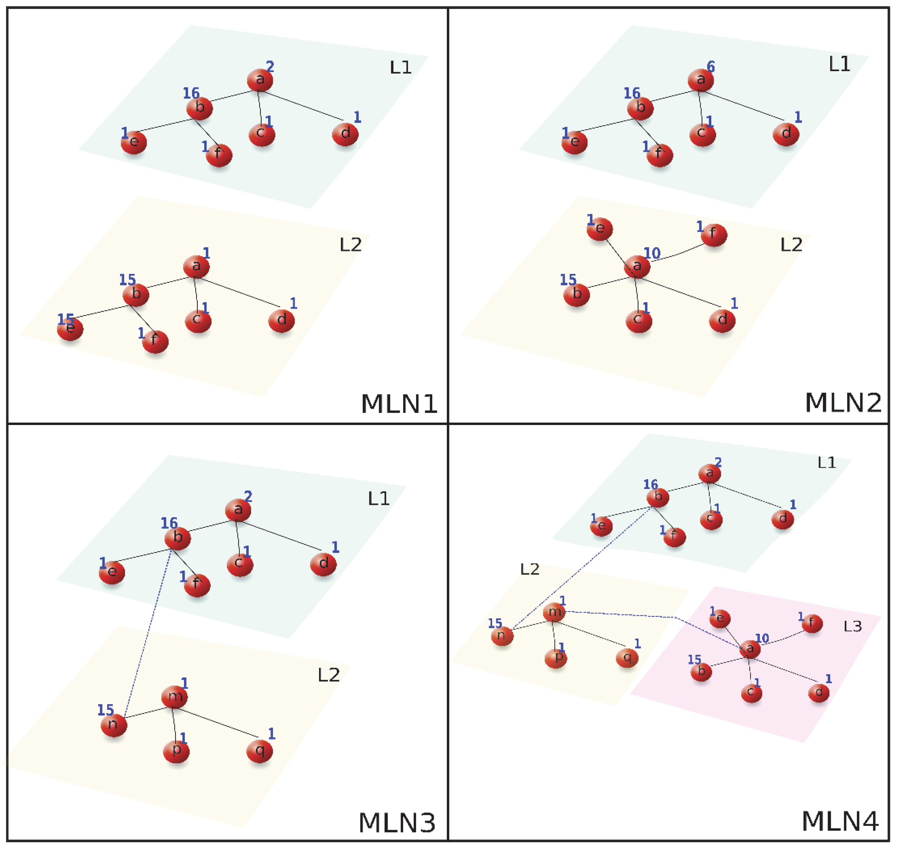
• Section 2 describes the mathematical model used to obtain the new centrality measure called the “corner centrality” of nodes in a multilayer network. To help readers understand the model, we have illustrated it with a toy example.
• In Section 3, we applied the model to different multilayer networks. For this, we selected three experiments to test the utility of the corner centrality measure.
• Section 4 presents the main conclusions of the paper and new research lines.

2. Mathematical Model for the Corner Centrality of Nodes in a Multilayer Network

We consider that a multilayer network $\mathcal{G}$ is composed of a set of layers $\left\{G_1,G_2,\dots ,G_M\right\}$. Every layer $G_i=\left(X_i,E_i\right)$ is a directed simple graph with $X_i=\left\{e_{i1},e_{i2},\dots ,e_{i{N}_i}\right\}$ being the set of nodes, and with $E_i=\left\{\left(e_{il},e_{jk}\right)\right\}$ being the set of edges such that $l\in \left\{0,1,\dots ,N_i\right\}$ and $k\in \left\{0,1,\dots ,N_j\right\}$ with $N_i$ and $N_j$ being the number of nodes in the graphs $G_i$ and $G_j$, respectively. Different examples of multilayer networks are shown in Figure 1.

Additionally, every node $u$ in a layer $L$ has an initial importance value $i_L\left(u\right)$. For example, in Figure 1, in the multilayer network $MLN1$, the $a$ node in layer one has an importance of 2, while in layer two it has a value of 1. This type of situation can be seen in a team project, when a researcher has a more relevant contribution in one task while in other tasks, the importance of that researcher is not as high.

A node should be perceived with more relative importance in a layer if its importance is higher than the importance of the nodes in its neighborhood in that layer. In this way, we can define the relative importance of a node $u$ in the layer $L$ as:

$$I_L\left(u\right)={\sum }_{\forall v\in Neighbou{r}_L\left(u\right)}{i}_L\left(u\right)-i_L\left(v\right)$$

(1)

Equation (1) uses the intralinks defined in layer $L$.

On the other hand, we can also define the relative importance in other layers, separate from the layer of the node, by using the interlinks as:

$$I_L\left(u\right)={\sum }_{\forall v\in Neighbou{r}_L\left(u\right)}{i}_{L*}\left(u\right)-i_L\left(v\right)$$

(2)

with $L$ being different from the node’s layer $L_{*}$. In this case, Equation (2) uses the interlinks defined between the $L$ and $L_{*}$ layers. $L_{*}$ is defined as the target layer while $L$ is the reference layer.

For example, by using Equation (1) for the node $b$, in the multilayer network MLN3 of Figure 1, we obtained the relative importance $I_{L_1}\left(b\right)$, and by using Equation (2), we obtained the relative importance in the layer $L_2$, $I_{L_2}\left(b\right)$.

The relative importance of a layer is normalized across the nodes to obtain a mean and standard deviation value of 0 and 1, respectively.

Finally, when we analyze the multilayer network, the relative global importance of a node will be higher if high relative importance is met in every layer for that node. In this case, we can define the relative global importance of a node as:

$$I\left(u\right)={\left({\sum }_{i=0}^M{I}_{L_i}\left(u\right)\right)}^2$$

(3)

In Figure 1 in MLN1, the importance for node $a$ would be: $I\left(a\right)={(I_{L_1}\left(a\right)+I_{L_2}\left(a\right))}^2$.

To simplify, we are going to suppose that we have a multilayer network with only two layers: $L_1$ and $L_2$. Then, Equation (3) would be:

$$I\left(u\right)={(I_{L_1}\left(u\right)+I_{L_2}\left(u\right))}^2$$

(4)

Additionally, if a node has a high global relative importance, this value must be transmitted across the nodes in its neighborhood, in the layer to which it belongs. In this sense, let $L_{*}$ be the target layer to which the node $u$ belongs; then, the $u$ node would have a high global relative importance across all the layers, and also, in layer $L_{*}$, the nodes that surround it would also have a high global relative importance:

$$C{C}_{L_{*}}\left(u\right)={\sum }_{v\in Neighbou{r}_{L_{*}}\left(u\right)\cup u}I\left(v\right)={\sum }_{v\in Neighbou{r}_{L_{*}}\left(u\right)\cup u}{(I_{L_1}\left(v\right)+I_{L_2}\left(v\right))}^2$$

(5)

In Equation (5), the summation that iterates over the neighbors of $u$ (including u) in the target layer adds to the relative importance of its neighbors in the target layer. Taking into account that ${(I_{L_1}\left(v\right)+I_{L_2}\left(v\right))}^2=I_{L_1}{\left(v\right)}^2+2I_{L_1}\left(v\right)I_{L_2}\left(v\right)+I_{L_2}{\left(v\right)}^2,$Equation (5) can be written in matrix form as:

$$C{C}_{L_{*}}\left(u\right)={\sum }_{v\in Neighbou{r}_{L_{*}}\left(u\right)\cup u}\left(\begin{array}{ll}1,\hfill & 1\hfill \end{array}\right)\left(\begin{array}{ll}{I}_{L_1}{(v)}^2\hfill & I_{L_1}\left(v\right)I_{L_2}\left(v\right)\hfill \\ \hfill & \hfill \\ I_{L_1}\left(v\right)I_{L_2}\left(v\right)\hfill & I_{L_2}{(v)}^2\hfill \end{array}\right)\left(\begin{array}{l}1\hfill \\ \hfill \\ 1\hfill \end{array}\right)$$

(6)

$C{C}_{L*}\left(u\right)$ can be rewritten as:

$$C{C}_{L_{*}}\left(u\right)=\left(\begin{array}{ll}1,\hfill & 1\hfill \end{array}\right)M\left(u\right)\left(\begin{array}{l}1\hfill \\ 1\hfill \end{array}\right)$$

(7)

where M is the structure tensor, and it is defined as:

$$M\left(u\right)={\sum }_{v\in Neighbou{r}_{L_{*}}\left(u\right)\cup u}\left(\begin{array}{ll}{I}_{L_1}{(v)}^2\hfill & I_{L_1}\left(v\right)I_{L_2}\left(v\right)\hfill \\ \hfill & \hfill \\ I_{L_1}\left(v\right)I_{L_2}\left(v\right)\hfill & I_{L_2}{(v)}^2\hfill \end{array}\right)$$

(8)

Note that the matrix M is derived from the differentials of the initial value of nodes’ importance in the target layer with respect to the neighboring nodes’ initial importance in the reference layers. For a number of layers $N$ bigger than two, the matrix $M$ is defined as:

$$M\left(u\right)={\sum }_{v\in Neighbou{r}_{L_{*}}\left(u\right)\cup u}\left(\begin{array}{llll}{I}_{L_1}{(v)}^2\hfill & I_{L_1}\left(v\right)I_{L_2}\left(v\right)\hfill & \dots \hfill & I_{L_1}\left(v\right)I_{L_N}\left(v\right)\hfill \\ \hfill & \hfill & \hfill & \hfill \\ ⋮\hfill & \ddots \hfill & \hfill & \hfill \\ I_{L_N}\left(v\right)I_{L_1}\left(v\right)\hfill & I_{L_N}\left(v\right)I_{L_2}\left(v\right)\hfill & \dots \hfill & I_{L_N}{(v)}^2\hfill \end{array}\right)$$

(9)

Equation (8) can be rewritten as:

$$M\left(u\right)=\left(\begin{array}{ll}{\sum }_{v\in Neighbou{r}_{L_{*}}\left(u\right)\cup u}{I}_{L_1}{(v)}^2\hfill & {\sum }_{v\in Neighbou{r}_{L_{*}}\left(u\right)\cup u}{I}_{L_1}\left(v\right)I_{L_2}\left(v\right)\hfill \\ {\sum }_{v\in Neighbou{r}_{L_{*}}\left(u\right)\cup u}{I}_{L_1}\left(v\right)I_{L_2}\left(v\right)\hfill & {\sum }_{v\in Neighbou{r}_{L_{*}}\left(u\right)\cup u}{I}_{L_2}{(v)}^2\hfill \end{array}\right)$$

(10)

To summarize the distribution of the relative importance of a node across different layers, we obtain the eigenvalues ${\lambda }_1$ and ${\lambda }_2$ of the matrix $M$.

In the case that ${\lambda }_2\ll {\lambda }_1$, the node has a high relative importance in layer one, but the relative importance in layer 2 is low. The opposite situation is achieved when ${\lambda }_1\ll {\lambda }_2$. In this paper, we want to obtain the nodes with highest relative importance across all layers, so for this we need ${\lambda }_1\approx {\lambda }_2$ (the two eigenvalues are large and similar in magnitude). Therefore, to obtain the minimum between ${\lambda }_1$ and ${\lambda }_2$, we use

$${\lambda }_{min}\approx \frac{{\lambda }_1{\lambda }_2}{{\lambda }_1+{\lambda }_2}=\frac{det\left(M\right)}{trace\left(M\right)}$$

(11)

where $det$ and $trace$ are the determinant and trace operators of the matrix M.

For example, if ${\lambda }_1\gg {\lambda }_2$, then $\frac{{\lambda }_1{\lambda }_2}{{\lambda }_1+{\lambda }_2}=\frac{{\lambda }_2}{\frac{{\lambda }_2}{{\lambda }_1}+1}\approx {\lambda }_2$. To summarize, our method generates a score for each node in layer $L_{*}$ as:

$$S_{L_{*}}\left(u\right)=\frac{det\left(M\left(u\right)\right)}{trace\left(M\left(u\right)\right)+ϵ}$$

(12)

where $ϵ$ is a small constant to avoid divisions by zero. The score $S_{L_{*}}$ defines the grade of the corner centrality of a node.

Algorithm 1 shows the steps to obtain the ranking proposed in this paper. The algorithm can be used for multilayer networks complying with the following conditions:

1.

The multilayer network can contain layers with the same set of nodes. In this case, the layers do not have interlinks between them.

2.

The multilayer network can contain layers with different nodes. In this case, the layers can be connected using interlinks between them.

3.

The multilayer network can contain interlinks and intralinks between layers.

Algorithm 1: corner centrality. Let $\mathcal{G}$ = {L1,L2,···, LM}, a multilayer network with M layers. Let L∗ be the target layer from $\mathcal{G}$.

1: for every node u in L∗, do 2:  for every layer L in G, do 3:   if u is in L, then 4:     obtain IL(u) by using Equation (1) ▷ by using intralinks within L 5:   else, if u is not in L, then 6:      obtain IL(u) by using Equation (2) ▷ by using interlinks between L∗ and L layers. 7:   end if 8:  end for 9: end for 10: for every layer L in G, do 11:   Normalize IL 12: end for 13: for every node u in L∗, do 14:  obtain the matrix M(u) by using Equation (9). ▷with only two layers by using Equation (10) 15:  obtain the score of the node SL∗(u) ▷by using Equation (12) 16: end for 17: Obtain the rank of every node in L∗ by sorting SL∗

With a multiplex network having every layer with the same set of nodes, without interlinks, the corner centrality value for every node is defined as the minimum value of corner centrality obtained across the layers. For example, in Figure 1, MLN2 obtains $S_{L_1}$ and $S_{L_2}$ for the node $a$, and the final score will be the minimum between $S_{L_1}$ and $S_{L_2}$.

The computational time of the algorithm would be:

1.

If the number of nodes n in every layer $L$ is bigger than the number of layers $M$, the computational time is $O\left(n^2\times M\right)$. Usually, $n\gg M$ and $O\left(n^2\times M\right)\approx O\left(n^2\right)$.

2.

If the number of nodes n in every layer $L$ is lower than the number of layers $M$, the computational time is $O\left(n\times M^{2.373}\right)$.

A more detailed analysis of the computational efficiency is described in Appendix A. Additionally, Appendix A describes the memory needs of the algorithm proposed.

A Toy Example

In this section, we will show the main steps of Algorithm 1 for the multilayer network MLN4 in Figure 1. If we want to obtain the corner centrality value for the nodes in layer $L_1$, then, according to Algorithm 1 $L_{*}$ will be $L_1$. Following the steps 1–9 in Algorithm 1, we obtained the relative importance of every node in $L_1$, analyzed by every layer (see

Table 1. Relative importance of every node in layer $L1$ from MLN4 in in Figure 1.

Relative Importance for Every Node
Node	${\mathit{I}}_{{\mathit{L}}_1}$	${\mathit{I}}_{{\mathit{L}}_2}$	${\mathit{I}}_{{\mathit{L}}_3}$
a	−12	0	31
b	44	1	5
c	−1	0	−9
d	−1	0	−9
e	−15	0	−9
f	−15	0	−9

):

To obtain the relative importance for layer $L_1$ (see column $I_{L_1}$ in Table 1) for every node in $L_1$, we used the intralink information. Thus, using a fixed node in the L1 layer, we consider its neighbors in $L_1$ and compute the differences of the initial value of importance between the node and its neighbors. In the same way, in layer $L_3$ we obtained the relative importance by using Equation (1) (see column $I_{L_3}$ in Table 1). However, for layer $L_2$, we used the interlink information to establish the relative importance of the nodes in $L_1$ for layer $L_2$ by using Equation (2) (see column $I_{L_2}$ in Table 1). In this case, the neighbors of the node in the $L_2$ layer are considered. For example, the node $b$ has a relative importance of 44 in the layer $L_1$. This value was obtained by adding:

$$I_{L_1}\left(b\right)=i_{L_1}\left(b\right)-i_{L_1}\left(a\right)+i_{L_1}\left(b\right)-i_{L_1}\left(e\right)+i_{L_1}\left(b\right)-i_{L_1}\left(f\right)=14+15+15$$

Concerning layer $L_2$ the relative importance of the node $b$ was obtained using the interlinks between layers $L1$ and $L2$:

$$I_{L_2}\left(b\right)=i_{L_1}\left(b\right)-i_{L_2}\left(n\right)=16-15=1$$

Additionally, to obtain the relative importance for the node $b$ in the layer $L_3$, we used the intralinks in layer $L_3$

$$I_{L_3}\left(b\right)=i_{L_3}\left(b\right)-i_{L_3}\left(a\right)=5$$

Analyzing Table 1, we can see that node $a$ has a high relative importance in layer $L_3$ but a very low importance in layers $L_1$ and $L_2$. Moreover, though node $a$ has a bigger initial importance than the importance of nodes $c$ and $d \mathrm{in}\mathrm{layer}{L}_1$, this relative importance stays low in regard to the importance of node $b$. Additionally, we see in Table 1 that for all the layers, node $b$ is essential.

In steps 11–12, we normalized the relative importance by subtracting the mean and divided by the standard deviation. The result of the normalization is shown in

Table 2. Normalized relative importance of every node in layer $L1$ from MLN4 in Figure 1.

Normalized Relative Importance for Every Node
Node	${\mathit{I}}_{{\mathit{L}}_1}$	${\mathit{I}}_{{\mathit{L}}_2}$	${\mathit{I}}_{{\mathit{L}}_3}$
a	−0.584	−0.447	2.098
b	2.142	2.236	0.338
c	−0.049	−0.447	−0.609
d	−0.049	−0.447	−0.609
e	−0.730	−0.447	−0.609

:

In steps 12–14, we calculated the corner centrality value for each node in layer $L_1$. In step 13, we obtained the matrix $M\left(u\right)$, which is $3\times 3$ and symmetrical. We must recall that the relative global importance of a node (see Equation (9)) must attend to its relative importance as well as the relative importance of the nodes in its neighborhood within layer $L_1$.

For the node $b$ in layer $L_1$, it is defined as:

$$M\left(b\right)=\left(\begin{array}{lll}{M}_{11}\left(b\right)\hfill & M_{12}\left(b\right)\hfill & M_{13}\left(b\right)\hfill \\ M_{21}\left(b\right)\hfill & M_{22}\left(b\right)\hfill & M_{23}\left(b\right)\hfill \\ M_{31}\left(b\right)\hfill & M_{32}\left(b\right)\hfill & M_{33}\left(b\right)\hfill \end{array}\right)$$

with

$$\begin{array}{l}{M}_{11}\left(b\right)=I_{L_1}{(b)}^2+I_{L_1}{(a)}^2+I_{L_1}{(e)}^2+I_{L_1}{(f)}^2\\ M_{12}\left(b\right)=M_{21}\left(b\right)=I_{L_1}\left(b\right)I_{L_2}\left(b\right)+I_{L_1}\left(a\right)I_{L_2}\left(a\right)+I_{L_1}\left(e\right)I_{L_2}\left(e\right)+I_{L_1}\left(f\right)I_{L_2}\left(f\right)\\ M_{13}\left(b\right)=M_{31}\left(b\right)=I_{L_1}\left(b\right)I_{L_3}\left(b\right)+I_{L_1}\left(a\right)I_{L_3}\left(a\right)+I_{L_1}\left(e\right)I_{L_3}\left(e\right)+I_{L_1}\left(f\right)I_{L_3}\left(f\right)\\ M_{22}\left(b\right)=I_{L_2}{(b)}^2+I_{L_2}{(a)}^2+I_{L_2}{(e)}^2+I_{L_2}{(f)}^2\\ M_{23}\left(b\right)=M_{32}\left(b\right)=I_{L_2}\left(b\right)I_{L_3}\left(b\right)+I_{L_2}\left(a\right)I_{L_3}\left(a\right)+I_{L_2}\left(e\right)I_{L_3}\left(e\right)+I_{L_2}\left(f\right)I_{L_3}\left(f\right)\\ M_{33}\left(b\right)=I_{L_3}{(b)}^2+I_{L_3}{(a)}^2+I_{L_3}{(e)}^2+I_{L_3}{(f)}^2\end{array}$$

Each value in the matrix evaluates the importance of each node in each layer, and further integrates the importance of the nodes in its neighborhood in the target layer.

Finally, we obtained the corner centrality measure by using Equation (12). For our example, the score was

$$\begin{array}{l}{S}_{L_1}\left(a\right)=0.345\hfill \\ S_{L_1}\left(b\right)=0.323\hfill \\ S_{L_1}\left(e\right)=1.75e-16\hfill \\ S_{L_1}\left(f\right)=1.75e-16\hfill \\ S_{L_1}\left(f\right)=-1.167e-17\hfill \\ S_{L_1}\left(d\right)=-1.16e-17\hfill \end{array}$$

This result shows that node $a$ had the highest centrality, followed by $b$. However, node $a$ was not the most important when we analyzed layer by layer. Nevertheless, adding the importance of the nodes in its neighborhood, the $a$’s importance grew because of the node’s importance to $b$.

3. Experimentation

3.1. Experiment 1: Biplex Networks

Here, we focus our method on a particular type of multilayer network: biplex networks. A biplex network is composed of two layers, and each layer only has intralinks. In this experiment, we wanted to test the goodness of our method compared to the APABI centrality [13] and Pagerank versatility [26]. The APABI method also uses an initial value of importance for the nodes in the multilayer network, but it is only applied to multiplex networks.

The Pagerank versatility can be applied to a multilayer network with intralinks and interlinks, but it does not utilize an initial value of importance of the nodes. Compared with this method, the corner centrality value takes the node’s degree as its initial value of importance. Next, we described the behavior of our method for the two different multiplex networks used in [13] and in [26].

3.1.1. Football Team

This experiment uses the example proposed in [13]. In this example, a biplex network was analyzed. The biplex is composed of two layers, each one with 20 nodes. Each node represents a player of a football team. The multilayer network has two layers that connect the players differently, and an undirected graph represents each layer. The first layer is constructed with the 20 nodes, and the relationships between the team members are analyzed from the point of view of their social or virtual relationships. Thus, two nodes are joined by an edge if they are related or linked through a social network. The initial importance of every node in this layer is the number of messages that each player receives from their teammates within a certain period. With the same 20 players, the second layer shows how the players relate to each other within the game. Thus, two players are connected in the graph if they pass the ball with some consistency during a match. The players’ initial importance is the number of games played in a season, seen in layer two.

Table 3. Data associated with the biplex network constructed by the team. This table was presented in [13].

Node	Social Network Links	Messages	Game Links	Games
1	2, 5, 7, 9, 16, 17, 19, 20	15	2, 4, 5, 6, 9, 12, 13, 14, 18, 19	33
2	1, 5, 7, 9, 20	9	1, 4, 8, 10, 13, 18, 19	26
3	7, 9, 11, 13, 14, 15, 17	12	4, 5, 6, 12, 14, 15, 17, 20	18
4	5, 9, 11, 14, 15, 16, 18, 20	19	1, 2, 3, 5, 6, 7, 8, 9, 10, 11, 12, 13, 14, 16, 17, 18, 20	32
5	1, 2, 4, 6, 7, 11, 12, 14, 18, 20	28	1, 3, 4, 6, 7, 8, 11, 14, 17, 19, 20	20
6	5, 7, 10, 20	7	1, 3, 4, 5, 8, 11, 12, 19	12
7	1, 2, 3, 5, 6, 8, 9, 18, 20	20	4, 5, 10, 11, 12, 13, 15, 16, 17, 18, 19, 20	32
8	7, 10, 12, 17, 18	7	2, 4, 5, 6, 9, 12, 13, 14, 18, 19	6
9	1, 2, 3, 4, 7, 10, 15, 18, 20	16	1, 4, 8, 10, 13, 16, 18, 19	18
10	6, 8, 9, 11, 13, 14, 15, 16, 18, 20	21	2, 4, 7, 9, 13, 15, 18, 19, 20	25
11	3, 4, 5, 10, 13, 18, 19, 20	14	4, 5, 6, 7, 12, 14, 15, 17, 20	24
12	5, 8, 14, 17, 20	8	1, 3, 4, 6, 7, 8, 11, 14, 19, 20	18
13	3, 10, 11, 15, 19, 20	11	1, 2, 4, 7, 8, 9, 10, 16, 17, 19, 20	6
14	3, 4, 5, 10, 12, 16, 18, 19	13	1, 3, 4, 5, 8, 11, 12, 19	26
15	3, 4, 9, 10, 13, 17, 20	11	3, 7, 10, 11, 16, 17, 20	38
16	1, 4, 10, 14, 17, 18, 19	14	4, 7, 9, 13, 15, 18, 19, 20	6
17	1, 3, 8, 12, 15, 16, 20	12	3, 4, 5, 7, 11, 13, 15, 18, 19	12
18	4, 5, 7, 8, 9, 10, 11, 14, 16, 19, 20	35	1, 2, 4, 7, 8, 9, 10, 16, 17, 19, 20	30
19	1, 11, 13, 14, 16, 18, 20	15	1, 2, 5, 6, 7, 8, 9, 10, 12, 13, 14, 16, 17, 18, 20	8
20	1, 2, 4, 5, 6, 7, 9, 10, 11, 12, 13, 15, 17, 18, 19	27	3, 4, 5, 7, 10, 11, 12, 13, 15, 16, 18, 19	25

shows the relationships for each node with other nodes (second column) when the social network connection is analyzed. The third column shows the number of messages received by a player in a period. The fourth column shows the relations between players in regard to the number of times they passed the ball to each other. Additionally, the fifth column is the number of games the player participated in during a season.

We applied our method to this multilayer network in order to obtain the corner centrality of each node. In this case, the multilayer is a multiplex network with the same set of nodes but without interlinks. In this case, the corner centrality value of every node is defined as the minimum value of corner centrality obtained across the layers. Additionally, the centrality measure defined for biplex multilayers in [13], called APABI, was used to compare it against our proposed corner centrality measure.

In

Table 4. APABI centrality [13] versus corner centrality.

	APABI		Corner Centrality
Nodes	Value	Rank	Value	Rank
1	0.05581	7	4.309008	10
2	0.03777	16	2.550988	16
3	0.04193	13	1.429319	20
4	0.06517	3	5.171486	4
5	0.06440	5	5.5569	3
6	0.02862	20	1.520039	19
7	0.06477	4	3.883725	11
8	0.03071	19	1.865937	18
9	0.04836	11	4.475997	7
10	0.05902	6	4.412212	9
11	0.05013	9	4.668175	6
12	0.03727	17	1.979066	17
13	0.03684	18	3.198247	14
14	0.04820	12	3.2216934	13
15	0.05085	8	3.068847	15
16	0.03781	15	4.450555	8
17	0.04033	14	3.3716	12
18	0.07590	2	6.405673	2
19	0.04838	10	4.726761	5
20	0.07775	1	8.063785	1

, the value of centrality and rank for each node for both the APABI method and our proposed method is presented. Additionally, in Figure 2, we illustrate the ranking for both methods.

The APABI centrality shows that the nodes classified as the highest values of centrality, the leaders of the group, were nodes 20 and 18. On the one hand, node 20 was third in messages received and eighth in the number of games in the season. On the other hand, node 18 was the node that received more messages but was fifth among players that played games in the season. Corner centrality also established that the nodes with the highest values of importance were, in first place, node 20, and in second place, node 18.

Our method generated a ranking similar to the APABI ranking. The main disadvantage of the APABI method is the tremendous amount of memory that it needs, as well as the method’s susceptibility to the parameter $\alpha$.

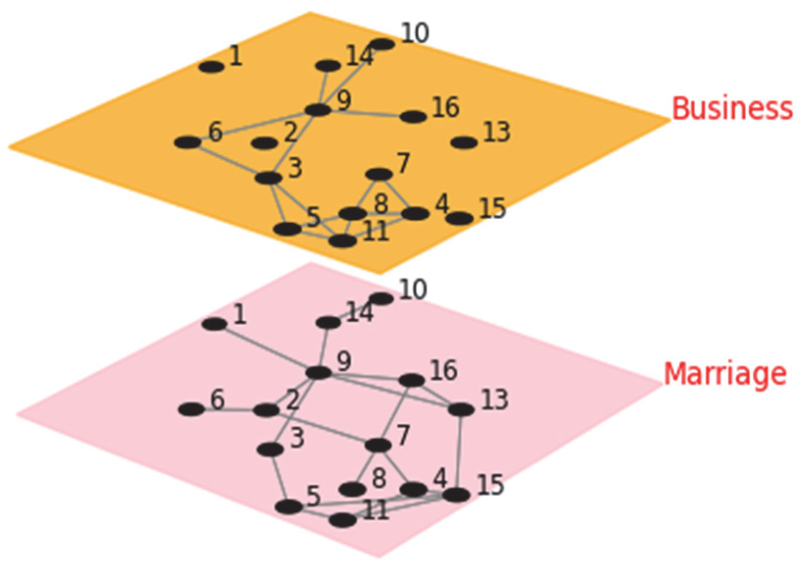
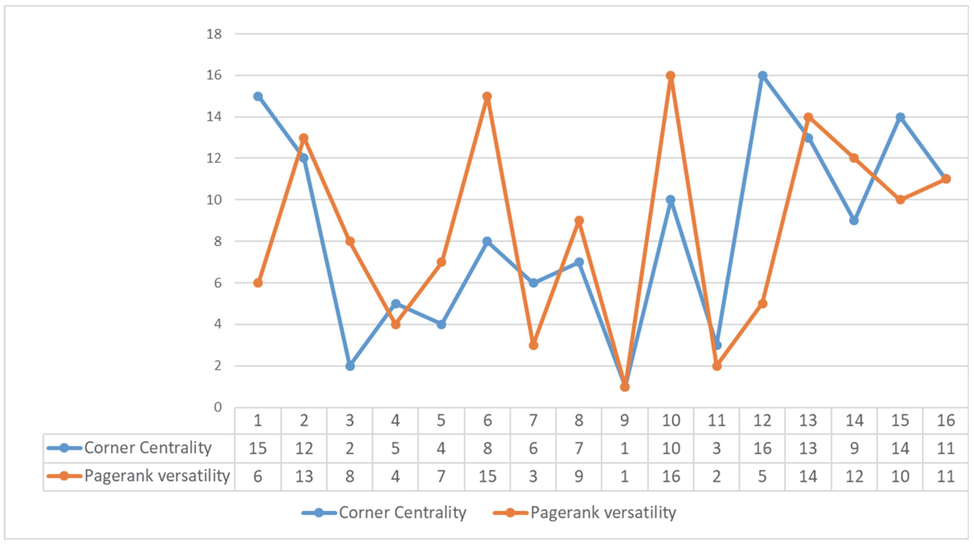
3.1.2. Florentine Families

In this experiment, we applied our method to the Florentine Families multiplex network [28]. This multiplex network is composed of two layers. One layer describes the business dealings between sixteen Florentine families in the XV century, and the other layer illustrates their alliances due to marriage. Figure 3 shows the married and business relationships between the Florentine families. In

Table 5. Corner centrality values and Pagerank versatility for the Florentine Families multiplex network.

		Corner Centrality		PageRank Versatility
Family Name	Node Id	Value	Rank	Value	Rank
Acciaiuol	1	0	15	0.8638167	6
Albizzi	2	0	12	0.8389033	13
Barbadori	3	0.87675385	2	0.8567245	8
Bischeri	4	0.250263979	5	0.8732232	4
Castellan	5	0.268755428	4	0.8557555	7
Ginori	6	0.083220632	8	0.8347692	15
Guadagni	7	0.223183775	6	0.8823537	3
Lambertes	8	0.109123972	7	0.8561786	9
Medici	9	1.229130987	1	1	1
Pazzi	10	0.041761825	10	0.830739	16
Peruzzi	11	0.278145671	3	0.8975903	2
Pucci	12	0	16	0.8638167	5
Ridolfi	13	0	13	0.8370955	14
Salviati	14	0.071072416	9	0.8374698	12
Strozzi	15	0	14	0.8496274	10
Tornabuon	16	0.025402425	11	0.8430032	11

, the code associated with the name of every family member is presented. To apply the corner centrality measure to this network, we assigned the node’s degree value as the node’s initial importance value in every layer. The method was then compared to the Pagerank versatility [26].

In Table 5 and Figure 4, the value and ranking of the corner centrality and Pagerank versatility methods are shown. For both methods, the Medici family (node 9 in Figure 4) was the node with the highest centrality value. Unlike PageRank versatility, the corner centrality method assigns a zero value to a node with an initial value of importance equal to zero in at least one layer. This is so because corner centrality looks for those nodes that maintain high importance throughout all the layers. It is a logical concept, for example, when we need an expert in different fields or a peace mediator in the different countries of a conflict.

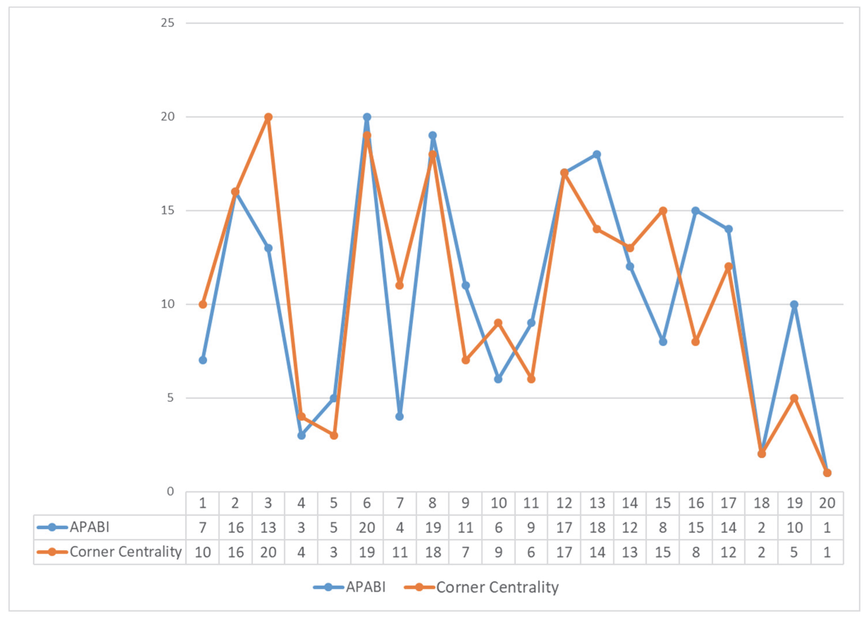
3.2. Experiment 2: Scopus vs. Google Trend

In this experiment, our objective was to analyze the importance of a set of author’s keywords. The set comes from a corpus of 69,000 documents as a result of a search in the Web of Science, using “Computer Science” as the search criteria but without applying any filters to the documents, either for type or area, to obtain the academic literature that discusses computer science but is not limited exclusively to this area.

We obtained two values for each keyword in this dataset: Scopus and Google. According to the Scopus Database, the Scopus value refers to the number of articles that contain specific keywords. Thanks to the Scopus value, we can obtain information about how frequently researchers use a keyword.

Concerning the Google value, we used the information provided by Google Trends to extract the global popularity of a term. We used trends data from 2020 to 2021. The Google value can help us to understand the social popularity of a keyword and the use of that keyword outside the world of academia. We built our dataset by using the unofficial PyTrends API.

To obtain the value for global popularity, the average popularity of the results for each of the 250 countries for which Google provides information was calculated. Then, the Scopus search API was used to find the number of articles that contained a particular word so as to obtain the Scopus value.

Many authors’ keywords were not presented in Scopus or Google Trend. In this case, the author keyword was erased. Thus, the dataset of keywords consisted of 27,704 words.

In this experiment, we built a multiplex network with the author’s keywords as the nodes. Thus, we would say that a link existed between two keywords if they appeared in the same paper. The multiplex layer had two layers. The layers had the same nodes and same links, but the initial importance of every node was the Google Trend score in the first layer and the Scopus score in the second layer.

Let $M{N}_{ak}$ be this multiplex network. To compare our centrality score, corner centrality, with APABI centrality [13], we obtained different subnetworks from $M{N}_{ak}$. The number of nodes for the subnetworks were $\left\{100,150,200,\dots 1000\right\}$. For each size, we generated a set of thirty subnetworks from $M{N}_{AK}$, where the nodes were chosen randomly. In

Table 6. Comparison between APABI centrality and corner centrality. For each set of networks (row), the number of nodes, the Spearman’s Correlation Rank mean value, and the standard deviation across the set are shown. Additionally, the mean values of the p-value and standard deviations are presented. Every set had 30 networks with the number of nodes given in the first column. The nodes were chosen from the MN_AK multiplex network.

Nodes	Spearman’s Correlation	Rank-Order	p-Value
	Mean	Std	Mean	Std
100	0.604	0.065	0.000	0.000
150	0.691	0.041	0.000	0.000
200	0.683	0.039	0.000	0.000
250	0.673	0.036	0.000	0.000
300	0.705	0.017	0.000	0.000
350	0.697	0.028	0.000	0.000
400	0.729	0.022	0.000	0.000
450	0.753	0.02	0.000	0.000
500	0.752	0.018	0.000	0.000
550	0.769	0.014	0.000	0.000
600	0.758	0.024	0.000	0.000
650	0.769	0.022	0.000	0.000
700	0.763	0.015	0.000	0.000
750	0.756	0.019	0.000	0.000
800	0.753	0.02	0.000	0.000
850	0.772	0.013	0.000	0.000
900	0.756	0.022	0.000	0.000
950	0.769	0.021	0.000	0.000
1000	0.765	0.025	0.000	0.000

, we computed the mean value of Spearman’s Correlation Rank between corner centrality and the APABI method for each set, and we show the p-value of the correlation. A p-value close to 0 was obtained for every set. Therefore, a strong correlation exists between the corner centrality and APABI methods.

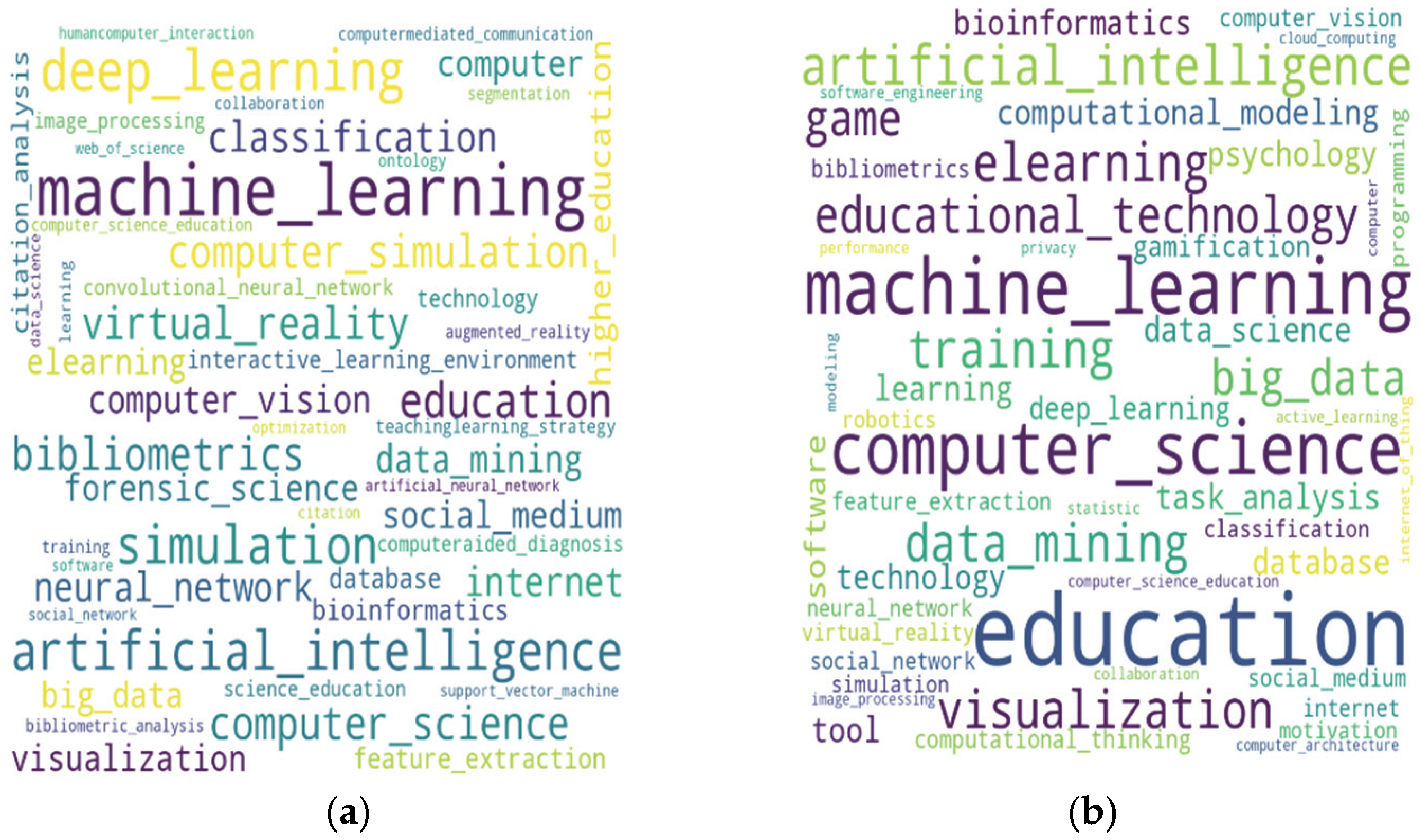
3.3. Experiment 3: Author Keywords vs. KeyWords plus Keywords

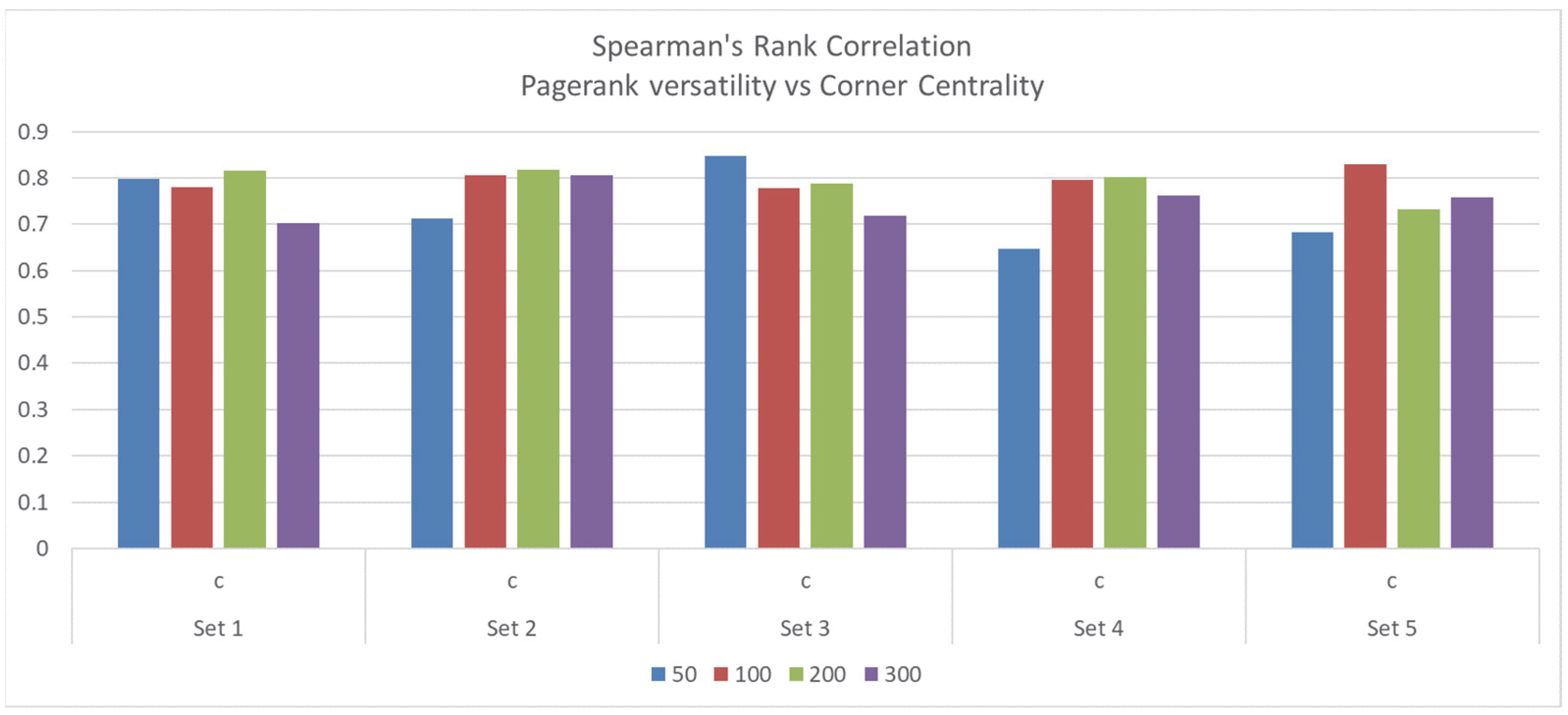
In this experiment, we wanted to obtain the corner centrality value of a set of author keywords using the relationship with the KeyWords Plus keywords from Web of Knowledge. Typically, authors select keywords, so we will call these words “author keywords”. However, it is more likely that authors do not have the freedom to choose keywords and automatic algorithms, and so predefined categories are used instead [29]. KeyWords Plus is one such alternative to author keywords. KeyWords Plus keywords are automatically generated from the titles of the articles that are referenced in a paper. According to [30], KeyWords Plus tries to reduce the problems generated by letting authors select their own keywords.

In the same way as Experiment 2, we obtained a set of author keywords from a corpus of 69,000 documents as a result of a search in Web of Science, using “Computer Science” as the search criteria but without applying any filters to the documents, either for type or area, to obtain the academic literature that discusses computer science but is not limited exclusively to this area. The set of author’s keywords was composed of 48,115 words, and the set of KeyWords Plus keywords contained 24,040 words. In this multilayer network, we had two layers. The first layer was composed of the author keywords as nodes, and between the nodes, a link existed if they appeared in the same paper. The initial importance of the nodes was the number of papers in which the author keywords appeared. In the second layer, the nodes were the KeyWords Plus keywords.

Similarly to the other experiments, the nodes had an initial importance equal to the number of papers where they appeared. In this second layer, two nodes were connected if they were in the same paper. Additionally, between nodes in layer 1 (author keywords) and nodes in the second layer (KeyWords Plus), a link could exist if they shared the same paper. Our aim in this multilayer was to obtain the corner centrality value of the set of author keywords. In this case, an author keyword would have a higher centrality if the relative importance was higher in the layer of author keywords and the layer of KeyWords Plus keywords.

In Figure 5a, the 50 authors’ keywords that appeared in the highest number of papers are presented. Moreover, the 50 author’s keywords with the highest corner centrality are on Figure 5b. In these word clouds, the size of the word is related to the value given. Therefore, the ranking given by corner centrality distinguishes between the words with high importance, such as education (first place), machine learning (second place), and computer science (third place).

Likewise, we obtained the KeyWords Plus keywords with the highest centrality and compared them with the KeyWords Plus keywords most frequently used in the papers. Thus, in Figure 6a, the 50 KeyWords Plus keywords with the highest frequency are shown, and on Figure 6b, the 50 KeyWords Plus keywords with the highest values of corner centrality are shown.

Validation

To validate the corner centrality measure, we compared it with the Pagerank versatility method [26]. However, the Pagerank versatility method has restrictions on the amount of memory that a multilayer needs. Thus, we generated different subnetworks from the author keywords and KeyWords Plus keywords (AK-KP multilayer network). All of them were undirected, containing intralinks, interlinks, and two layers: author keywords and KeyWords Plus keywords. The multilayer networks had 50, 100, 200, and 300 nodes. Additionally, for every set of nodes, we obtained five multilayer networks. This dataset can be downloaded at https://www.kaggle.com/datasets/jorgechamorropadial/author-keywords-keywordsplus (accessed on 13 September 2022).

For our method, the initial value of the importance of every node is its degree, recalling that a link between two keywords means that they appeared in the same paper.

We created five sets of multilayer networks composed of 50, 100, 200, and 300 nodes. Every multilayer network obtained the node’s ranking given by the Pagerank versatility method and the corner centrality measure. To test the correlation between the two rankings, we applied Spearman’s Rank Correlation, finding the correlation ($c$) and how likely or probable it was that any observed correlation was due to chance ($p$).

In Figure 7 and

Table 7. Spearman’s Rank Correlation between the centrality measures of the Pagerank versatility and corner centrality (c) and p-value (p).

	Set 1		Set 2		Set 3		Set 4		Set 5
$\#\mathit{N}\mathit{o}\mathit{d}\mathit{e}\mathit{s}$	c	$\mathit{p}$	c	$\mathit{p}$	c	$\mathit{p}$	c	$\mathit{p}$	c	$\mathit{p}$
50	0.7977	4 × 10−12	0.7130	6 × 10−9	0.8475	8 × 10−15	0.6463	3 × 10−7	0.6835	4 × 10−8
100	0.7798	1 × 10−21	0.8048	6 × 10−24	0.7784	1 × 10−21	0.7951	5 × 10−23	0.8295	1 × 10−26
200	0.815	6 × 10−49	0.8171	2 × 10−49	0.7878	1 × 10−43	0.8026	2 × 10−46	0.7327	6 × 10−26
300	0.7019	7 × 10−46	0.8066	4 × 10−70	0.7190	5 × 10−49	0.7627	2 × 10−58	0.7582	2 × 10−57

, the correlation ($c$) and the p-value ($p$) are presented. Thus, for $Set1$, we obtained a minimum correlation of 0.70 for the network with 300 nodes and 0.82 for the network with 200 nodes. For $Set2$, the minimum value of correlation was achieved for the network of 50 nodes with a value of 0.71, and the maximum value was obtained for the network with 200 nodes (0.82). For $Set3$, we obtained a minimum and maximum correlation of 0.72 and 0.85, respectively. For $Set4$, we obtained the values of 0.64 and 0.80 as the minimum and maximum values of correlation, respectively. Finally, for $Set5$, we achieved a minimum value of 0.68 and a maximum value of 0.82. For all cases shown in Table 7, the probability that an observed correlation was due to chance($p$) is close to zero. The average correlation ($\widehat{c}$) and the average probability p-value ($\widehat{p}$) across the multilayer networks with the same number of nodes is shown in

Table 8. $\widehat{c}$ = Average Spearman’s Rank Correlation between the centrality measures: Pagerank versatility and corner centrality, across the multilayer networks with the same number of nodes. $\widehat{p}$ = Average p-value (p) across the multilayer networks with the same number of nodes.

	50	100	200	300
$\widehat{c}$	0.7376	0.7975	0.7911	0.7497
$\widehat{p}$	8 × 10−8	5 × 10−22	1 × 10−35	1 × 10−46

.

4. Conclusions

In this paper, we have presented a new method with which to obtain the centrality of nodes in a multilayer network. The method can be applied to multilayer networks with nodes that have an initial value of importance. If the initial value of importance is not given, the method will use the degree of the node.

Our method deals with multilayer networks, which can be multiplex networks and multilayer networks with interlinks. The primary constraint is that the nodes in different layers with interlinks have an initial value of importance with information of the exact nature related to their source. For example, consider a multilayer network with different layers, one per area, and the nodes are authors publishing in that area. The initial importance of the nodes (authors) can be their h-index. A paper published by different authors generates a link between them in the network. The authors can be in the same area (layer) or different areas (different layers), but the nodes’ initial value of importance in different layers with interlinks between them is the same information (h-index value).

Two hypotheses support this method: (1) A node will be more important when all the layers establish that the node has a high relative importance; and (2) the centrality of a node will be higher if nodes in its neighborhood are essential. To meet these two hypotheses, we presented a new algorithm with a low computational time. It is also important to note that the memory needs are very low compared to other algorithms, and the algorithm does not need to adjust any input parameter.

To test the performance of our method, we compared it with the APABI centrality and the Pagerank versatility methods by carrying out three experiments. The first experiment was applied to two small biplex networks. In both biplexes, the nodes in both layers were the same, but the links were different.

The second experiment was also applied to a set of biplex networks with several nodes per layer. This experiment used the relations between author keywords in the context of scientific papers. We aimed to obtain the author’s keywords with the highest centrality in this multiplex network. We characterized the nodes with Scopus and Google Trends values.

For the third experiment, we used author keywords and KeyWords Plus keywords (from Web of Knowledge), which was defined as a multilayer network with interlinks between two layers. Additionally, in this experiment, we wanted to determine the author’s keywords with the highest centrality. In this case, the keywords were characterized by the number of papers in which they appeared. The results of the corner centrality method were then compared with the results of the Pagerank versatility method.

In every experiment, the results were outstanding.

As a line of future research, we would like to analyze the possibility of weighing the importance given by every layer to the nodes in the target layer. Furthermore, we want to study how the corner centrality of a node is affected when the importance of the nodes in the neighborhood is weighed.

5. Source Code

The source code of our experiments can be found in a GitHub repository located at https://github.com/rosadecsai/Corner-Centrality.git (accessed on 13 September 2022).

References

1. Newman, M. Networks: An Introduction; Oxford University Press: Oxford, UK, 2010. [Google Scholar]
2. Applegate, D.L.; Bixby, R.M.; Chvátal, V.; Cook, W.J. The Traveling Salesman Problem; Princeton University Press: Princeton, NJ, USA, 2006; ISBN 978-0-691-12993-8. [Google Scholar]
3. Gabow, H.N.; Galil, Z.; Spencer, T.; Tarjan, R.E. Efficient algorithms for finding minimum spanning trees in undirected and directed graphs. Combinatorica 1986, 6, 109. [Google Scholar] [CrossRef]
4. Cellai, D.; Bianconi, G. Multiplex networks with heterogeneous activities of the nodes. Phys. Rev. E 2016, 93, 32302. [Google Scholar] [CrossRef] [PubMed]
5. de Domenico, M.; Solé-Ribalta, A.; Cozzo, E.; Kivelä, M.; Moreno, Y.; Porter, M.; Gómez, S.; Arenas, A. Mathematical Formulation of Multilayer Networks. Phys. Rev. X 2013, 3, 041022. [Google Scholar] [CrossRef]
6. Bazzi, M.; Lucas, G.; Jeub, S.; Arenas, A.; Howison, S.D.; Porter, M.A. A framework for the construction of generative models for mesoscale structure in multilayer networks. Phys. Rev. Res. 2020. [Google Scholar] [CrossRef]
7. Moreno, Y.; Perc, M. Focus on multilayer networks. New J. Phys. 2019, 22, 10201. [Google Scholar] [CrossRef]
8. Gosak, M.; Markovič, R.; Dolenšek, J.; Rupnik, M.S.; Marhl, M.; Stožer, A.; Perc, M. Network science of biological systems at different scales: A review. Phys. Life Rev. 2018, 24, 118–135. [Google Scholar] [CrossRef] [PubMed]
9. Wu, J.; Pu, C.; Li, L.; Cao, G. Traffic dynamics on multilayer networks. Digit. Commun. Netw. 2020, 6, 58–63. [Google Scholar] [CrossRef]
10. Pi, B.; Zeng, Z.; Feng, M.; Kurths, J. Evolutionary multigame with conformists and profiteers based on dynamic complex networks. Chaos Interdiscip. J. Nonlinear Sci. 2022, 32, 023117. [Google Scholar] [CrossRef]
11. Stella, L.; Martínez, A.P.; Bauso, D.; Colaneri, P. The role of asymptomatic infections in the COVID-19 epidemic via complex networks and stability analysis. SIAM J. Control Optim. 2022, 60, S119–S144. [Google Scholar] [CrossRef]
12. Agryzkov, T.; Oliver, J.L.; Tortosa, L.; Vicent, J.F. An algorithm for ranking the nodes of an urban network based on the concept of PageRank vector. Appl. Math. Comput. 2012, 219, 2186–2193. [Google Scholar] [CrossRef]
13. Agryzkov, T.; Curado, M.; Pedroche, F.; Tortosa, L.; Vicent, J.F. Extending the Adapted PageRank Algorithm Centrality to Multiplex Networks with Data Using the PageRank Two-Layer Approach. Symmetry 2019, 11, 284. [Google Scholar] [CrossRef]
14. McGee, F.; Ghoniem, M.; Melançon, G.; Otjacques, B.; Pinaud, B. The State of the Art in Multilayer Network Visualization. Comput. Graph. Forum 2019, 38, 125–149. [Google Scholar] [CrossRef]
15. Lv, Y.; Huang, S.; Zhang, T.; Gao, B. Application of Multilayer Network Models in Bioinformatics. Front. Genet. 2021, 12, 664860. [Google Scholar] [CrossRef] [PubMed]
16. Kinsley, A.C.; Rossi, G.; Silk, M.J.; VanderWaal, K. Multilayer and Multiplex Networks: An Introduction to Their Use in Veterinary Epidemiology. Front. Vet. Sci. 2020, 7, 596. [Google Scholar] [CrossRef] [PubMed]
17. Sola, L.; Romance, M.; Criado, R.; Flores, J.; Garcia del Amo, A.; Boccaletti, S. Eigenvector centrality of nodes in multiplex networks. Chaos 2013, 23, 33131. [Google Scholar] [CrossRef] [PubMed]
18. Iacovacci, J.; Rahmede, C.; Arenas, A.; Bianconi, G. Functional Multiplex PageRank. Eur. Lett. 2016, 116, 28004. [Google Scholar] [CrossRef]
19. Sharifi, S.S.; Barati, H. A method for routing and data aggregating in cluster-based wireless sensor networks. Int. J. Commun. Syst. 2021, 34, e4754. [Google Scholar] [CrossRef]
20. Oliveira, E.M.; Ramos, H.S.; Loureiro, A.A. Centrality-based routing for wireless sensor networks. In Proceedings of the 3rd IFIP Wireless Days Conference 2010, Venice, Italy, 20–22 October 2010; pp. 1–5. [Google Scholar]
21. Kenyeres, M.; Kenyeres, J. Comparative Study of Distributed Consensus Gossip Algorithms for Network Size Estimation in Multi-Agent Systems. Future Internet 2021, 13, 134. [Google Scholar] [CrossRef]
22. Halu, A.; Mondragon, R.; Panzarasa, P.; Bianconi, G. Multiplex PageRank. PLoS ONE 2013, 8, e78293. [Google Scholar] [CrossRef]
23. Solé-Ribalta, A.; De Domenico, M.; Gómez, S.; Arenas, A. Centrality Rankings in Multiplex Networks. In Proceedings of the 2014 ACM Conference on Web Science, Bloomington, IN, USA, 23–26 June 2014; ACM: New York, NY, USA, 2014; pp. 149–155. [Google Scholar]
24. Bianconi, G. Multilayer Networks. Structure and Functions; Oxford University Press: Oxford, UK, 2018. [Google Scholar]
25. Harris, C.; Stephens, M. A Combined Corner and Edge Detector. In Proceedings of the 4th Alvey Vision Conference, Manchester, UK, 31 August–2 September 1988; pp. 147–151. [Google Scholar]
26. de Domenico, M.; Solé-Ribalta, A.; Omodei, E.; Gómez, S.; Arenas, A. Ranking in interconnected multilayer networks reveals versatile nodes. Nat. Commun. 2015, 6, 6868. [Google Scholar] [CrossRef] [PubMed] [Green Version]
27. Brin, S.; Page, L. The Anatomy of a Large-Scale Hypertextual Web Search Engine. Comput. Netw. ISDN Syst. 1998, 30, 107–117. [Google Scholar] [CrossRef]
28. Padgett, J.F.; Ansell, C.K. Robust Action and the Rise of the Medici, 1400–1434. Am. J. Sociol. 1993, 98, 1259–1319. [Google Scholar] [CrossRef]
29. Lu, W.; Liu, Z.; Huang, Y.; Bu, Y.; Li, X.; Cheng, Q. How do authors select keywords? A preliminary study of author keyword selection behavior. J. Informetr. 2020, 14, 101066. [Google Scholar] [CrossRef]
30. Garfield, E.; Sher, I.H. KeyWords Plus. Algorithmic Derivative Indexing. J. Am. Soc. Inf. Sci. 1993, 44, 298–299. [Google Scholar] [CrossRef]
31. Aho, A.V.; Hopcroft, J.E.; Ullman, J.D. The Design and Analysis of Computer Algorithms, Theorem 6.6; Addison-Wesley: Boston, MA, USA, 1974; p. 241. [Google Scholar]
Figure 1. Examples of different multilayer networks. MLN1 is a multilayer network with two layers that have the same nodes and links. However, the nodes in each layer have different levels of importance. MLN2 has two layers with the same nodes but different links, and the nodes have different levels of importance. MLN3 has two layers with different nodes and links and the two layers are connected by links. MLN4 has three layers.
Algorithms 15 00336 g001
Figure 2. Comparison between APABI ranking and corner centrality ranking for the Football Team multiplex network. In this figure, we can see the degree of consensus between APABI and corner centrality. According to APABI, the leaders of the group are nodes 20 and 18, showing an overlap with the corner centrality measure.
Algorithms 15 00336 g002
Figure 3. This figure illustrates the Florentine Families multiplex network. For the experiment described in Section 3.1.2, we built a multiplex network using information about business alliances in one layer, and marriage in the other one.
Algorithms 15 00336 g003
Figure 4. Comparison between Pagerank versality ranking and corner centrality ranking for the Florentine Families multiplex network. In this comparison, we wanted to check the level of consensus between corner centrality and PageRank versatility measures. Both measures selected node 9 as the one with the highest centrality values.
Algorithms 15 00336 g004
Figure 5. Two word clouds that compare results of the corner centrality value with the 50 most frequent keywords. (a): The 50 author keywords with the highest frequency. (b): The 50 author keywords with the highest corner centrality value.
Algorithms 15 00336 g005
Figure 6. Two word clouds that compare results of the corner centrality value with the 50 most frequent keywords. (a): The 50 KeyWords Plus keywords with the highest frequency. (b): The 50 Keywords Plus keywords with the highest corner centrality value.
Algorithms 15 00336 g006
Figure 7. Spearman’s Rank Correlation between the centrality measures: Pagerank versatility and corner centrality. The multilayer networks compared have 50, 100, 200, and 300 nodes. For every set of nodes, we generated five multilayer networks and obtained the correlation and significance values ( c and p ) for each.
Algorithms 15 00336 g007