Parallel Computing of Edwards—Anderson Model

Abstract

A scheme for parallel computation of the two-dimensional Edwards—Anderson model based on the transfer matrix approach is proposed. Free boundary conditions are considered. The method may find application in calculations related to spin glasses and in quantum simulators. Performance data are given. The scheme of parallelisation for various numbers of threads is tested. Application to a quantum computer simulator is considered in detail. In particular, a parallelisation scheme of work of quantum computer simulator.

1. Introduction

The Edwards—Anderson model was proposed by Edwards and Anderson in 1975 to describe the physics of spin glass [1,2]. The model represents a set of spins arranged at the nodes of the lattice. Each spin can take on a value of $+1$ or $-1$ (or the direction up or down in some one dimensional isotopic space). All adjacent spins interact with each other. The interaction energy of one pair is calculated by the formula

$$\begin{array}{c}\hfill E=\sum _{<i,j>}{J}_{ij}{s}_i{s}_j,\end{array}$$

(1)

where the sum symbol with the index $<i,j>$ denotes the summation over all adjacent lattice nodes, $J_{ij}$ is a coupling constants between spins, taking values $+1$ or $-1$ with equal probability for bimodal distribution and any values with probability

$$\begin{array}{c}\hfill P\left(J_{ij}\right)=\frac{1}{\sqrt{2\pi }{J}_0}{e}^{-\frac{J_{ij}}{2J_0}}\end{array}$$

(2)

for Gaussian distribution.

Spin glasses have a complex energy landscape and property of ultrametricity [3]. The spin glass model is used in taxonomy, classification problems, information theory, biology, bioinformatics, protein folding and freezing [3], in neural networks, in assessments performance evaluation of quantum computers and in optimisation problems. As neural network theory has evolved, particularly since the creation of the Hopfield network [4,5,6], Restricted Boltzmann machine [7] and deep Boltzmann machine [8] interest in spin glasses has increased significantly. In the Hopfield network, finding an image from a distorted input image is reduced to the problem of finding metastable states with maximum correlation of the input image with the trained one. The set of local minima of states corresponds to the set of memorized images. By constructing properly the coupling constants between spins it is possible to control the size of the barriers between states, the number of local minimums, width of valleys, etc. [9] This explains the many publications devoted to the analysis of metastable states and methods for counting their number [10,11,12]. Knowing the physics of spin glasses allows us to control performance, error rate and data processing capacity of the neural network. A development of the Hopfield network is the Boltzmann machine, the operation of which has a probabilistic nature. The Boltzmann machine allows us to overcome relatively small local minima and stay at deeper ones. This makes its operation more stable and efficient in practical applications.

One important practical application of the ground state search methods is testing quantum computers. Ground state search algorithms can serve as a benchmark for quantum computers. For example, DWave computers are adapted to solve the problem of finding the ground state of spin glasses [13,14]. Due to the imperfect technology, errors occur in quantum computers that lead to incorrect results. Thus, the problem arises of constructing an a priori known ground state for testing a quantum computer [15]. An interesting approach to tackle this problem is given in [16]. It is based on reducing the problem of solving a system of linear algebraic equations (with algebraic operations modulo two) to the problem of searching for the ground state. It is worth noting that besides quantum computers other analogue devices are under development to solve the optimisation problem of Edwards—Anderson models [15,16,17].

The theory of spin glass is closely related to optimization problems, in particular to the problem of the equality of P and NP classes. An exact polynomial-time method for finding the ground state has not yet been found. But there are many probabilistic approaches to solving this problem. We can mention here the Monte Carlo methods [18,19], simulated annealing algorithms [20,21], parallel tempering and multicanonical Monte Carlo sampling [22].

It is worth mentioning the exact method based on the Pfaffian calculation and modular arithmetic methods [23]. It is also capable of working with lattices up to size 100 × 100.

Hartmann and others have developed many approaches for ground state computation based on the genetic algorithms [24], the cluster algorithms [25], and the shortest path finding algorithms linking frustrated clusters [26]. The latter computes in polynomial time and is able to deal with lattices up to 1448 × 1448.

In [27] the method based on Pfaffian matrices is presented. It’s able to compute lattices up to 3000 × 3000 with free boundary conditions in one direction. The method uses the FKT theorem.

In the paper the exact method for obtaining the ground state of the Edwards—Anderson model is presented using high-performance parallel computations. Although the algorithm is exponential in time, it is nevertheless able to perform calculations on a 40 × 40 lattice computing cluster in time of the order of days when parallelised across 64 threads, using about 400 GB of RAM. The limit lattice size available to the algorithm is smaller than in some of the works mentioned above. Nevertheless, the proposed approach has several advantages.

• The polynomial increase in computation time (without increasing the amount of RAM) while fixing the size of one side and increasing the size of the other, which makes it possible to compute 40 × 100, 40 × 1000, 40 × 10,000 lattices etc. This feature is not available to the method presented in [23].
• The method is exact.
• The possibility to handle different distributions (not only bimodal). It is possible to take into account impurities and heterogeneities.
• The ease of implementation.

The important issue of the computer simulations is the possibility to parallelise the task because it gives an opportunity to use the power of modern high performance systems and, consequently, to calculate more complex and larger lattices of spins. The main material of the article will be devoted to parallelisation.

The method allows us to find both the ground state energy and ground state spin configurations. Free boundary conditions are used in the model. For periodic or toroidal boundary conditions parallelisation will be trivial. In the latter case we would have just a set of completely independent calculations of parts of the partition functions. In the end we would sum up all parts taking into account the additivity of partition functions.

The article is organized as follows: the first section provides the description of the method and the parallelisation scheme. The second section provides performance data for bimodal distribution. Further we give the conclusions.

2. Algorithm

To find the minimum energy it is necessary to enumerate all possible states of the lattice spins, calculate their energies and compare them with each other. In order not to calculate it every time, one can calculate once the energies of states of a subsystem (part of the initial system) with given boundaries, and then extend the subsystem by adding spins to it. Knowing the boundary state makes it possible to calculate the change of energy of the ground state when adding spins. So $E\to E+\Delta E$. Expanding the subsystem by adding one spin at each step until the initial given system is achieved, we compute at each step a new minimum energy. The calculated energy of the ground state at the last step will be the final answer. This approach is quite widespread and is used, in particular, in the transfer matrix method in the calculation of the Ising model [28] and quantum many-body problem models [29,30]. Further, let’s describe the parallelisation scheme, preliminarily introducing some notations and formalizing the task.

Let a lattice have size $L_y$ × $L_x$. The above described energy calculation scheme for filling the spins of one lattice row (let the system expand line by line) can be represented as follows

$$\begin{array}{c}\hfill \left(\begin{array}{c}E{(s_1=-1,s_2=-1,\cdots ,s_{L_x}=-1)}_{m-1,L_x}\\ E{(s_1=+1,s_2=-1,\cdots ,s_{L_x}=-1)}_{m-1,L_x}\\ \cdots \\ E{(s_1=+1,s_2=+1,\cdots ,s_{L_x}=+1)}_{m-1,L_x}\end{array}\right)\stackrel{\mathrm{add}{s}_{m,1}}{\to }\left(\begin{array}{c}E{(s_1=-1,s_2=-1,\cdots ,s_{L_x}=-1)}_{m,1}\\ E{(s_1=+1,s_2=-1,\cdots ,s_{L_x}=-1)}_{m,1}\\ \cdots \\ E{(s_1=+1,s_2=+1,\cdots ,s_{L_x}=+1)}_{m,1}\end{array}\right)\end{array}$$

(3)

$$\stackrel{\mathrm{add}{s}_{m,2}}{\to }\cdots \stackrel{\mathrm{add}{s}_{m,L_x}}{\to }\left(\begin{array}{c}E{(s_1=-1,s_2=-1,\cdots ,s_{L_x}=-1)}_{m,L_x}\\ E{(s_1=+1,s_2=-1,\cdots ,s_{L_x}=-1)}_{m,L_x}\\ \cdots \\ E{(s_1=+1,s_2=+1,\cdots ,s_{L_x}=+1)}_{m,L_x}\end{array}\right).$$

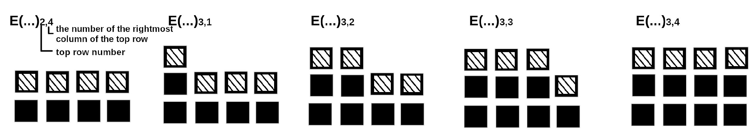
From the scheme one can see that all values of the minimum energy of the subsystem with a given boundary consisting of $L_x$ spins are written in vector-columns. Each column component corresponds to a given subsystem boundary. The state of the boundary is given by the set $(s_1,s_2,\cdots ,s_{L_x})$. The column has $2^{L_x}$ components. Thus all states of the upper boundary are covered. The bottom two indices $y,x$ to the right after the bracket $E{(\cdots )}_{y,x}$ denote the subsystem consisting of y rows with x spins in the top y line. We extend it at each step, adding one spin from left to right, so these indices allow us to understand which subsystem we are dealing with at the current step. The notation system is given for the lattice with $L_x=4$ in Figure 1.

After filling one line, one should repeat the process for the next line until the original system is obtained.

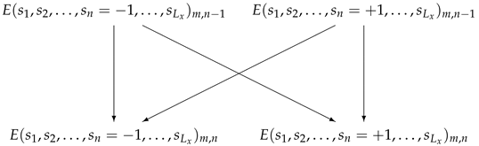
Let us consider in details the calculation of E. Knowing the boundary and all possible states of the added spin $s_{m,n}$ (the indices m and n denote the vertical and horizontal coordinates, respectively) one can calculate the minimum value of E of two subsystems with boundaries differing in the state of only one spin, by the formula  

$$\begin{array}{c}E{(s_1,s_2,\cdots ,s_n=-1,\cdots ,s_{L_x})}_{m,n}=\hfill \\ =min(E{(s_1,s_2,\cdots ,s_n=-1,\cdots ,s_{L_x})}_{m,n-1}+\Delta E({(s_1,s_2,\cdots ,s_n=-1,\cdots ,s_{L_x})}_{m,n-1},s_{m,n}=-1),\\ \hfill E{(s_1,s_2,\cdots ,s_n=+1,\cdots ,s_{L_x})}_{m,n-1}+\Delta E({(s_1,s_2,\cdots ,s_n=+1,\cdots ,s_{L_x})}_{m,n-1},s_{m,n}=-1))\end{array}$$

(4)

and

$$\begin{array}{c}E{(s_1,s_2,\cdots ,s_n=+1,\cdots ,s_{L_x})}_{m,n}=\hfill \\ =min(E{(s_1,s_2,\cdots ,s_n=-1,\cdots ,s_{L_x})}_{m,n-1}+\Delta E({(s_1,s_2,\cdots ,s_n=-1,\cdots ,s_{L_x})}_{m,n-1},s_{m,n}=+1),\\ \hfill E{(s_1,s_2,\cdots ,s_n=+1,\cdots ,s_{L_x})}_{m,n-1}+\Delta E({(s_1,s_2,\cdots ,s_n=+1,\cdots ,s_{L_x})}_{m,n-1},s_{m,n}=+1)).\end{array}$$

(5)

Here $\Delta E$ is the energy change after spin addition, the first argument $\Delta E$ in brackets denotes the boundary state, the second one is the state of the added spin. Let us explain for better understanding that in the expressions (4) and (5) the values of spins $s_1,s_2,s_3,\cdots ,s_n,\cdots ,s_{L_x}$ (excepting $s_n$) have the same values for a given boundary to the left and to the right of the equality sign. In the process of calculations we run over all states the boundaries. Thus, Formula (4) will be applied $2^N/2$ times (as well as (5)) to calculate $2^N$ new E when adding spin at position of the column number n. The minimum energy of the subsystem of the new set for one boundary state is calculated using only two values of E of the previous set, distinguished by a single spin state with the column number n (to a given column with the number n a spin is added):

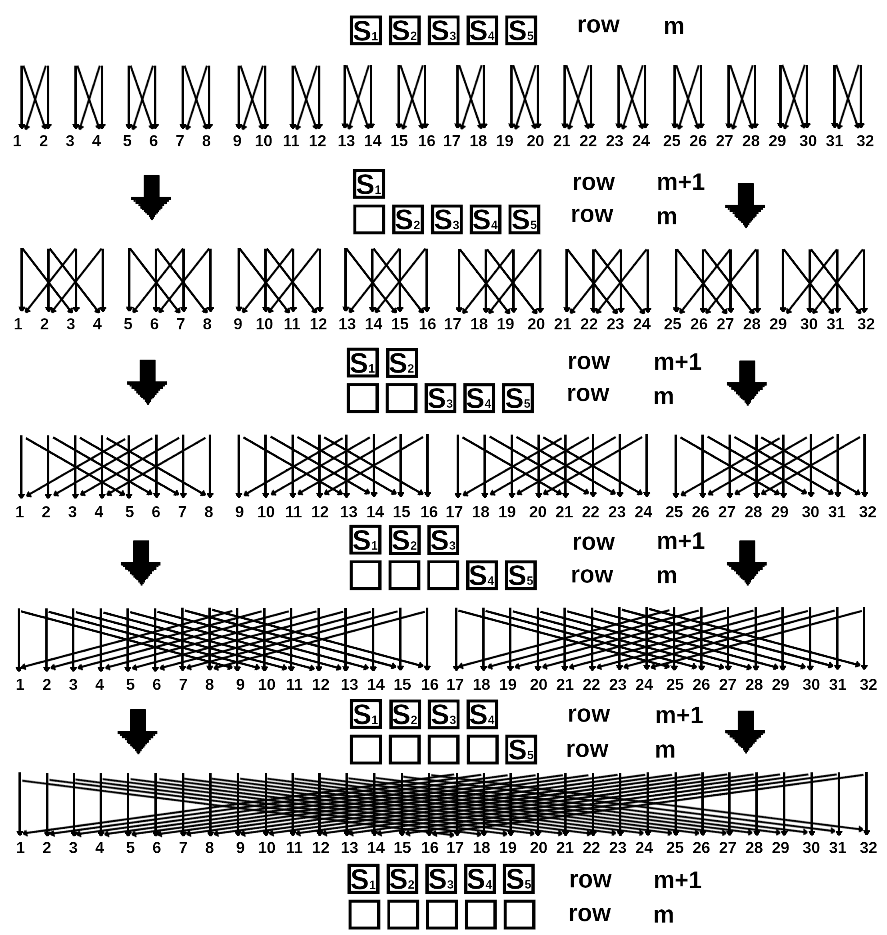
Thus, to calculate a new set of minimal energies, all states must be grouped into pairs differing by the spin state at position n. After adding the next spin already at the n+1 column position, the configurations of the spin boundaries of each pair will differ only by the state of n + 1 spin. An example of the pairing of a set of boundary spins for a lattice with $L_x=5$ for all five steps of row filling is given in Figure 2. Two-headed arrows signify data exchange (swap). One part takes up the place of the other part which occupies in turn the place of the first part.

The pair energies of this set E are determined by the energies of only one pair of the previous set. The number of boundary spin states is $2^5$, so the number of pairs will be $2^4$. Listing 1 gives an example of pseudocode for splitting the states of the boundary into pairs.

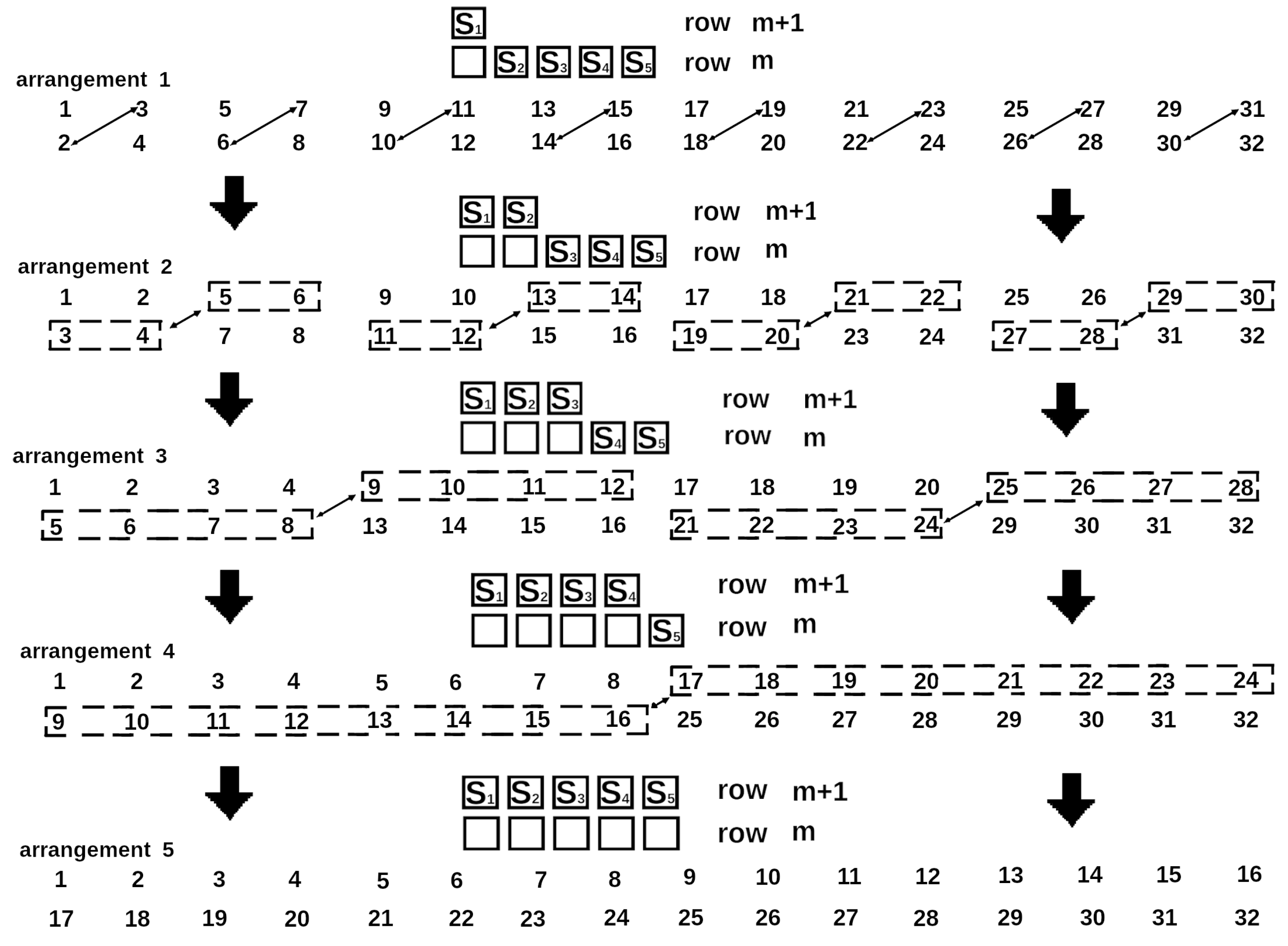
According to the diagram in Figure 2, two nested loops are needed to split the elements into pairs. In the listing, these loops are executed with the use of variables $index\_out$ and $index\_in$. The variables $state1$ and $state2$ store the state numbers of the boundary of the respective paired states. The energies of the states are stored in the array $E[\cdots ]$. It can be seen that as the column number increases, the distance between the spin numbers increases as well. Due to the fact that the links change when a spin is added, it is clear that in the parallelisation scheme one will need to do transitions of data between threads in a non-trivial way. To understand how this should be done, let’s rewrite the parallelisation scheme in a different way. Namely we can write the spin state numbers of the pair together (one under the other), as done in Figure 3.

Listing 1. Pseudocode of enumeration rows and columns, splitting states into pairs, calculating new energy minima.

for (int row=0;  row < Ly;  row++)

{

int max_step_out=(2^Lx)/2, max_step_in=1;

int state1=0,  state2=max_step_in;

for (int col=0;  col < Lx;  col++)

{

for (int index_out=0; index_out < max_step_out; index_out++)

{

for (int index_in=0; index_in < max_step_in; index_in++)

{

state1=index_out*max_step_in*2+index_in;

state2=state1+max_step_in;

.....

calc_E(...)

//    (E[state1],  E[state2])  =>  (E[state1],  E[state2])

.....

}

}

max_step_out=max_step_out/2;   max_step_in=max_step_in*2;

//

}

}

Listing 1. Pseudocode of enumeration rows and columns, splitting states into pairs, calculating new energy minima.

for (int row=0;  row < Ly;  row++)

{

int max_step_out=(2^Lx)/2, max_step_in=1;

int state1=0,  state2=max_step_in;

for (int col=0;  col < Lx;  col++)

{

for (int index_out=0; index_out < max_step_out; index_out++)

{

for (int index_in=0; index_in < max_step_in; index_in++)

{

state1=index_out*max_step_in*2+index_in;

state2=state1+max_step_in;

.....

calc_E(...)

//    (E[state1],  E[state2])  =>  (E[state1],  E[state2])

.....

}

}

max_step_out=max_step_out/2;   max_step_in=max_step_in*2;

//

}

}

If we wanted variables with paired states storing energy to be in adjacent positions of memory, then we would move the data each time (while adding spin) as shown by the arrows in Figure 3. E.g., in Figure 2 in the second row the configuration 1 must interact with the configuration 3, 2 with 4 and etc. Exchanging the locations of data in memory according the arrows in the first row on the scheme of Figure 3 we get pairs 1 and 3, 2 and 4 on the adjacent cells of the memory.

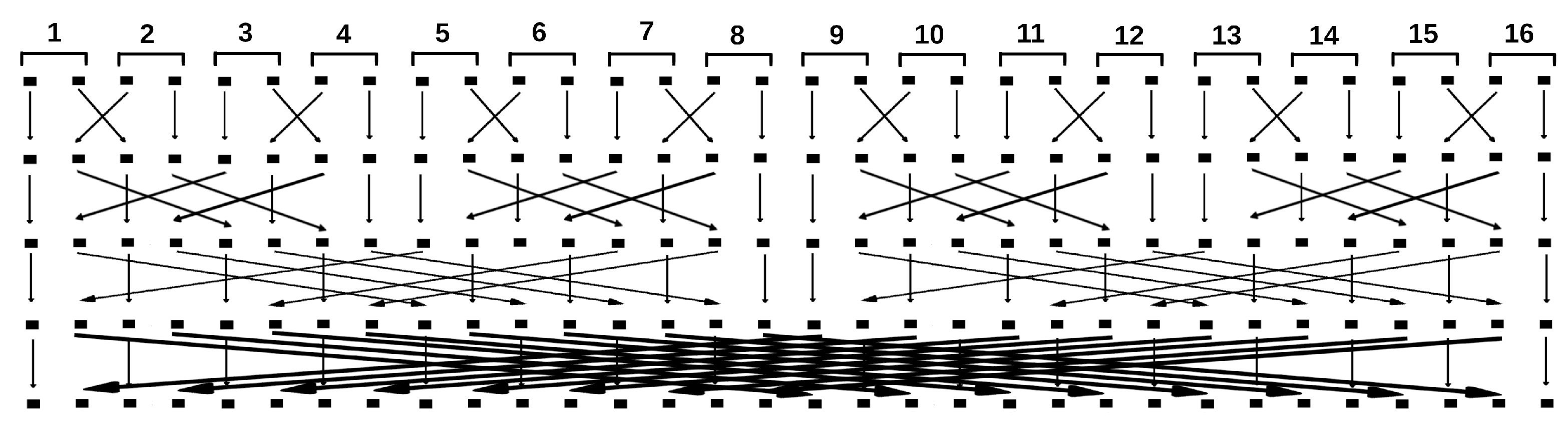
From the diagram in Figure 3 one can understand how to move data between threads when doing parallelisation. As the column number increases, the difference of the pairing state numbers increases. So, starting from a certain $n_{exch}$ column number at the position of which spin must be added, it is necessary to move data between threads according to the Figure 3. One can see that in the blocks with data circled by a dotted line in the figure, the state numbers are ordered. This makes it possible to construct the following data exchange scheme. When dealing with subsystems with the number of top row spins $n<n_{exch}$, no data is moved within the thread. The splitting of elements into pairs and energy calculation is done in Listing 1. Then, when the column number n is such that $n\ge n_{exch}$, we do a data exchange between streams so that the paired elements are arranged as in Figure 3. The scheme of data exchange between threads will look as shown in Figure 4. It should be emphasized that the scheme in Figure 4 literally the same as one as in Figure 3. Pulling numbers with their arrows and lining them up in one row we get the scheme in Figure 4. Also each 2 areas (pair of E) of the memory are joined into one thread (they are enumerated).

This circuit is made for 16 threads. For 16 streams 4 exchange operations will be performed to sequentially form four new subsystems. If data with a pair of E is located within one thread after data, the energy will be calculated according to the scheme of Figure 2. The code for calculating the energy minima within each thread is given in Listing 2. The paired elements do not change their occupying locations when adding a spin with number n horizontally such that $n\ge n_{exch}$. The listing demonstrates this process by calculating the variables $state1$ and $state2$.

Listing 2. Pseudocode of splitting states into pairs, calculating new energy minima for subsystems with column number n ≥ n_exch. Nthr is the number of thread. startstate1 and startstate2 are the numbers of start states stored inside the memory blocks and transferred by threads.

int max_step_in=(2^Lx)/Nthr/2;

int state1=0,  state2=max_step_in;

for (int index_in=0; index_in < max_step_in; index_in++)

{

state1=startstate1+max_step_in;

state2=startstate2+max_step_in;

.....

calc_E(...)

//    (E[state1],  E[state2])  =>  (E[state1],  E[state2])

.....

}

Listing 2. Pseudocode of splitting states into pairs, calculating new energy minima for subsystems with column number n ≥ n_exch. Nthr is the number of thread. startstate1 and startstate2 are the numbers of start states stored inside the memory blocks and transferred by threads.

int max_step_in=(2^Lx)/Nthr/2;

int state1=0,  state2=max_step_in;

for (int index_in=0; index_in < max_step_in; index_in++)

{

state1=startstate1+max_step_in;

state2=startstate2+max_step_in;

.....

calc_E(...)

//    (E[state1],  E[state2])  =>  (E[state1],  E[state2])

.....

}

Recall that Figure 4 corresponds to only 2 E per thread. Since according to the Figure 3 scheme the data within blocks (they are surrounded by a dashed line) are arranged in order, to facilitate the calculation of state numbers, the initial state numbers in the blocks can also be transmitted in the array of energy values. It can be seen that in the diagram of Figure 4 data exchange between threads can be done using two nested loops, as was done in Listing 1. Based on the diagram in Figure 4, namely by observing how groups of threads vary in size, we can construct the whole system of data exchange between all threads. Thus, the pseudocode calculating the energy minima for different subsystems is given in Listing 3.

Listing 3. Pseudocode for rows and columns enumeration, memory exchange between threads, energy calculation for cases col < n_exch and col ≥ n_exch. After completion of building each row, the memory locations are moved in the opposite direction. The code does not consider the calculation of the subsystem consisting of the lowest row only, because in this case there is no data exchange between threads. In the latter case, its calculation is trivial. The data exchange between threads is performed using two nested cycles on variables thrd_num_out and thrd_num_in. When calculating the energy by the subprogram calc_E(...), it is necessary to dispatch as arguments the array of energy values, the number of the column, the length of the side Lx.

for (int row=1;  row < Ly;  row++)

{

for (int col=0;  col < n_exch;  col++)

{

for (int thrd_num=0; thrd_num < thrd_amount;  thrd_num++)

{calc_E(min_E_array, col, Lx);}

}

int  interval_amount_of_thrds=2, interval_amount_of_thrds_div_2=1,

amount_of_bunchs_of_connected_thrds=N_thrd/2;

for  (int col=n_exch;  col < Lx;  col++)

{

// mem swap     ======  v

for (int thrd_num_out=0;  thrd_num_out <

amount_of_bunchs_of_connected_thrds;  thrd_num_out++)

{

for (int thrd_num_in=0;  thrd_num_in < interval_amount_of_thrds_div_2;  thrd_num_in++)

{

int thrd_num_1=thrd_num_out*interval_amount_of_thrds+thrd_num_in,  thrd_num_2=thrd_num_1+interval_amount_of_thrds_div_2;

swap_mem(min_E_array, thrd_num_1, thrd_num_2);      //  !  !          !                      !

!        !

}

}

// mem swap     ======  ^

for (int thrd_num=0; thrd_num < N_thrd;  thrd_num++)

{calc_E(min_E_array, col, Lx);}

}

...

mem_restore(...);

...

}

Listing 3. Pseudocode for rows and columns enumeration, memory exchange between threads, energy calculation for cases col < n_exch and col ≥ n_exch. After completion of building each row, the memory locations are moved in the opposite direction. The code does not consider the calculation of the subsystem consisting of the lowest row only, because in this case there is no data exchange between threads. In the latter case, its calculation is trivial. The data exchange between threads is performed using two nested cycles on variables thrd_num_out and thrd_num_in. When calculating the energy by the subprogram calc_E(...), it is necessary to dispatch as arguments the array of energy values, the number of the column, the length of the side Lx.

for (int row=1;  row < Ly;  row++)

{

for (int col=0;  col < n_exch;  col++)

{

for (int thrd_num=0; thrd_num < thrd_amount;  thrd_num++)

{calc_E(min_E_array, col, Lx);}

}

int  interval_amount_of_thrds=2, interval_amount_of_thrds_div_2=1,

amount_of_bunchs_of_connected_thrds=N_thrd/2;

for  (int col=n_exch;  col < Lx;  col++)

{

// mem swap     ======  v

for (int thrd_num_out=0;  thrd_num_out <

amount_of_bunchs_of_connected_thrds;  thrd_num_out++)

{

for (int thrd_num_in=0;  thrd_num_in < interval_amount_of_thrds_div_2;  thrd_num_in++)

{

int thrd_num_1=thrd_num_out*interval_amount_of_thrds+thrd_num_in,  thrd_num_2=thrd_num_1+interval_amount_of_thrds_div_2;

swap_mem(min_E_array, thrd_num_1, thrd_num_2);      //  !  !          !                      !

!        !

}

}

// mem swap     ======  ^

for (int thrd_num=0; thrd_num < N_thrd;  thrd_num++)

{calc_E(min_E_array, col, Lx);}

}

...

mem_restore(...);

...

}

Knowing the minimum energy for the given system and the energies for each state of boundary spins of the row with number $Ly$, one can obtain configurations of spins with the minimum energy by carrying out $Ly·Lx-1$ runs of the program, decreasing the number of spins by one each time and setting the upper boundary of the subsystem corresponding to the minimum energy or the current reduced lattice. This follows from the Formulas (4) and (5), where for $E{(s_1,s_2,\cdots ,s_n=-1,\cdots ,s_{L_x})}_{m,n}$ and $E{(s_1,s_2,\cdots ,s_n=+1,\cdots ,s_{L_x})}_{m,n}$ we assume the known values, and $E{(s_1,s_2,\cdots ,s_n=-1,\cdots ,s_{L_x})}_{m,n-1}$ and $E{(s_1,s_2,\cdots ,s_n=+1,\cdots ,s_{L_x})}_{m,n-1}$ are unknown. In calculating the energy minimum, we increase the subsystem each time, starting with the subsystem consisting of the lowest row. But when calculating the spin configuration corresponding to the energy minimum, we move “in the opposite direction”, decreasing the subsystem at each step and starting from the subsystem equal to the initial system.

3. Performance

In

Table 1. Performance of the parallel algorithm for fbc spin lattice calculation for 20 × 20, 25 × 25, 30 × 30, 35 × 35 lattices on 64 threads.

Calc. Number i	Lattice	Time ${\mathit{t}}_{\mathit{i}}$	Ratio of ${\mathit{t}}_{\mathit{i}}$ to ${\mathit{t}}_{\mathit{i}-1}$	Memory Size
1	20 × 20	81 ms		384 kb
2	25 × 25	4 s 282 ms	52.86	12 Mb
3	30 × 30	3 min 15 s	48.75	384 Mb
4	35 × 35	2 h 20 min	43.07	12 Gb

the performance parameters of the parallel algorithm of ground state search for 20 × 20, 25 × 25, 30 × 30, 35 × 35 lattices are given.

Parallelisation was performed for 64 threads (threads). The time relations are also given in the table. It can be seen that the times grow exponentially with the increasing linear size of the square lattice. Knowing the time ratios for the 35 × 35 and 40 × 40 lattices, equal to $43.07$, we can estimate the computation time of the 40 × 40 lattice. It will be approximately 5 h.

Further

Table 2. Performance of the parallel algorithm of fbc spin lattice calculation for 35 × 35, 50 × 35, 100 × 35, 250 × 35, 500 × 35 lattices on 64 threads.

Calc. Number i	$\mathit{Ly}$	Ratio of ${\mathit{Ly}}_{\mathit{i}}$ to ${\mathit{Ly}}_{\mathit{i}-1}$	Time ${\mathit{t}}_{\mathit{i}}$	Ratio of ${\mathit{t}}_{\mathit{i}}$ to ${\mathit{t}}_{\mathit{i}-1}$
1	35		2.33 h
2	50	1.4	3.46 h	1.49
3	100	2.0	6.89 h	1.99
4	250	2.5	17.17 h	2.49
5	500	2.0	35.00 h	2.03

shows the performance data of the lattice calculation algorithm with the fixed side length $Lx=35$ and different side lengths $Ly$.

Parallelisation was performed on 64 threads. The table shows that the time grows linearly with the increasing length of one side of the lattice.

To estimate the effectiveness of the parallelisation scheme, a series of calculations were carried out for 1, 2, 4, 8, 16, 32 and 64 threads. 25 × 25 and 28 × 28 lattices were considered. The data are given in

Table 3. Performance of the parallel algorithm of 25 × 25 and 28 × 28 lattices calculation for 1, 2, 4, 8, 16, 32 and 64 threads.

		25 × 25	25 × 25	28 × 28	28 × 28
Calc. Number i	Amount of Threads	${\mathit{t}}_{\mathit{i}}$	Ratio of ${\mathit{t}}_{\mathit{i}}$ to ${\mathit{t}}_{\mathit{i}-1}$	Time ${\mathit{t}}_{\mathit{i}}$	Ratio of ${\mathit{t}}_{\mathit{i}}$ to ${\mathit{t}}_{\mathit{i}-1}$
1	1	2 min 3 s		20 min 58 s
2	2	1 min 55 s	1.07	19 min 37 s	1.07
3	4	59 s	1.94	9 min 39 s	2.03
4	8	29 s	2.00	4 min 50 s	1.99
5	16	17 s	1.96	2 min 47 s	1.73
6	32	9 s	2.0	1 min 34 s	1.78
7	64	5 s	1.7	51 s	1.84

.

One can roughly accept that the running time depends on the size $Lx$ as $t\sim 2^{Lx}/N_{thrd}$ for $N_{thrd}$ threads. In this case we neglect the data transfer time. Thus, if $N_{thrd}$ increased by 2, the computation time will be reduced by 2. We can see from Table 3 that this ratio is more or less satisfied. Therefore, in our case the computational complexity is $2^{Lx}$ (NP-hard).

4. Use in a Quantum Computer Simulator

Further, we will show how to use the proposed scheme in a quantum simulator. Unitary operators in quantum computers can be represented as a product of 1-qubit and 2-qubit operators [31]. Therefore, to understand the principle of operation, it is sufficient to consider a 2-qubit quantum gate.

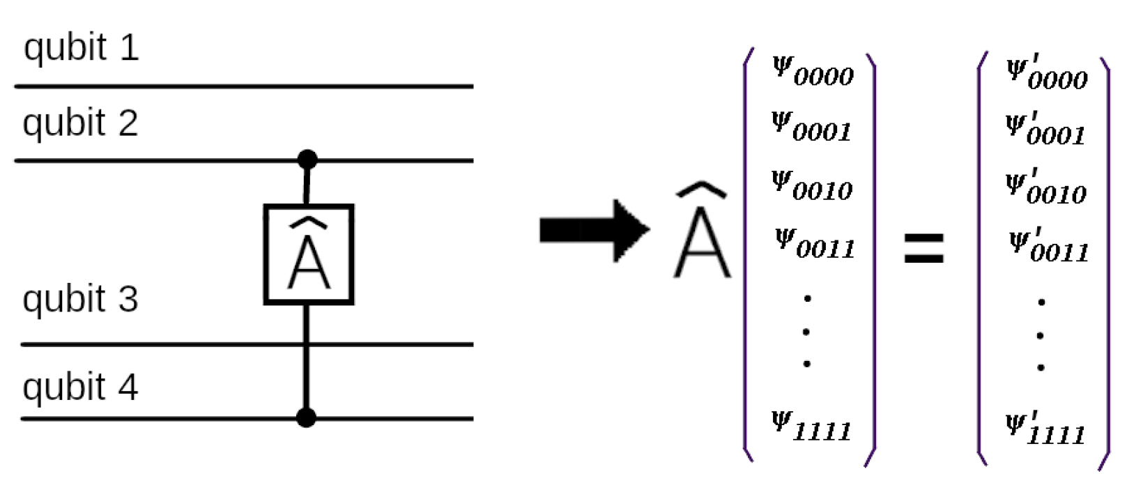
To reproduce an action of a quantum gate on n qubits in the common case we have to apply a $2^n$×$2^n$ matrix operator $\widehat{A}$ on the $2^n$ components of a vector in a $2^n$-dimensional Hilbert space (see [31]). Each component of a new vector-state is computed using 4 other components as input for a 2-qubit operator $\widehat{A}$. Let us a 2-qubit operator acts on qubits number p and number q. So in the result qubit and in 4 input ones all qubit states are the same except for the states with the numbers numbers p and q as it’s shown here

$$\begin{array}{c}\hfill \left(\begin{array}{c}{\mathsf{\Psi }}_{k_n,\cdots ,0,\cdots ,0,\cdots ,k_2,k_1}^{{}^{\prime }}\\ {\mathsf{\Psi }}_{k_n,\cdots ,0,\cdots ,1,\cdots ,k_2,k_1}^{{}^{\prime }}\\ {\mathsf{\Psi }}_{k_n,\cdots ,1,\cdots ,0,\cdots ,k_2,k_1}^{{}^{\prime }}\\ {\mathsf{\Psi }}_{k_n,\cdots ,1,\cdots ,1,\cdots ,k_2,k_1}^{{}^{\prime }}\end{array}\right)=\left(\begin{array}{cccc}{a}_{11}& a_{12}& a_{13}& a_{14}\\ a_{21}& a_{22}& a_{23}& a_{24}\\ a_{31}& a_{32}& a_{33}& a_{34}\\ a_{41}& a_{42}& a_{43}& a_{44}\end{array}\right)\left(\begin{array}{c}{\mathsf{\Psi }}_{k_n,\cdots ,0,\cdots ,0,\cdots ,k_2,k_1}\\ {\mathsf{\Psi }}_{k_n,\cdots ,0,\cdots ,1,\cdots ,k_2,k_1}\\ {\mathsf{\Psi }}_{k_n,\cdots ,1,\cdots ,0,\cdots ,k_2,k_1}\\ {\mathsf{\Psi }}_{k_n,\cdots ,1,\cdots ,1,\cdots ,k_2,k_1}\end{array}\right).\end{array}$$

(6)

So the problem is to find and match all groups of 5 components (1 output and 4 inputs) from the $2^n$ Hilbert space.

Applying the proposed approach of pairing elements we can find all groups of 5 elements to apply a 2-qubit operator to them. In the scheme in Figure 3 we can notice that after each addition of a spin in the resulting pairs the 2 spin states differ by only 1 number (0 or 1) in the binary representation. We can use it in quantum simulators.

The operation scheme of the algorithm can be clearly understood using the example of a quantum circuit of 4 qubits. Let us an operator $\widehat{A}$ act on the qubits number 2 and number 4. It’s shown in Figure 5.

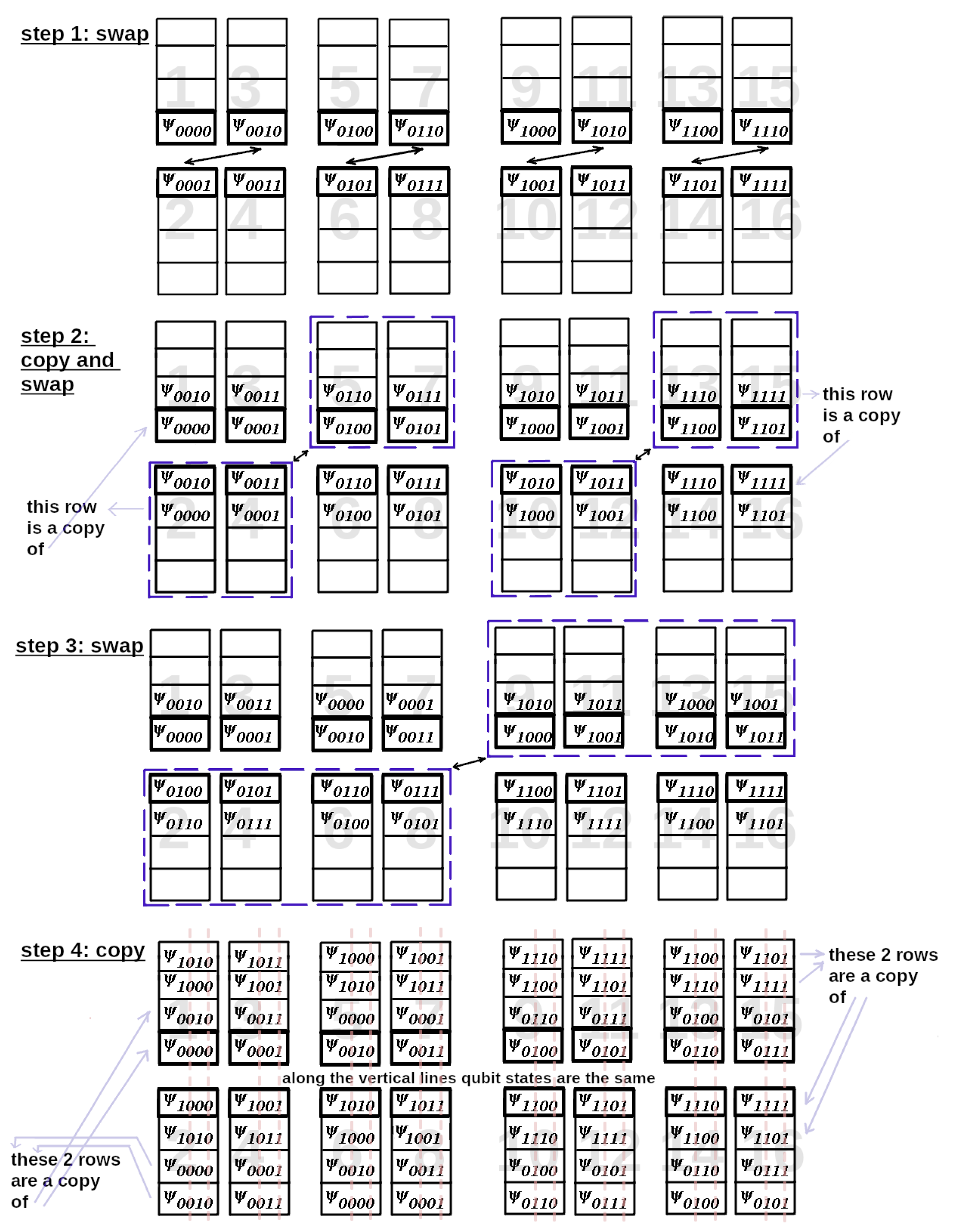
Next, we are going to reproduce the sequence of operations in Figure 3. Our goal is to calculate all components of $\overrightarrow{{\mathsf{\Psi }}^{{}^{\prime }}}$ which are linear combinations of components $\overrightarrow{\mathsf{\Psi }}$. Every component of $\overrightarrow{\mathsf{\Psi }}$ contains amplitudes and phases of the appropriate wave function. The whole scheme for 4-qubit is given in Figure 6 with the components of $\overrightarrow{{\mathsf{\Psi }}^{{}^{\prime }}}$ which are written in the binary representation.

Here we collect 4 input variables-components $\overrightarrow{\mathsf{\Psi }}$ in one place in the memory and match them with the components of $\overrightarrow{{\mathsf{\Psi }}^{{}^{\prime }}}$. In Figure 6 we get in each step pairs of states differing only by one qubit state. We must catch the components of $\overrightarrow{\mathsf{\Psi }}$ with different states of qubit 2 and qubit 4. As it’s seen in Figure 6 on steps 2 and 4 these qubit states are diferrent in every pair. Keeping this in mind, we can try to copy the pair as done in the diagram. Beforehand we allocate memory to store the additional data after copying. Thus, in step 3 we transmit already the pairs, not just one component (with only the state of the second qubit being different). In step 4, by copying pairs, we get exactly states with all 4 combinations of states of the qubits 2 and 4, but with the same states of the qubits 1 and 3. The big numbers denote memory locations.

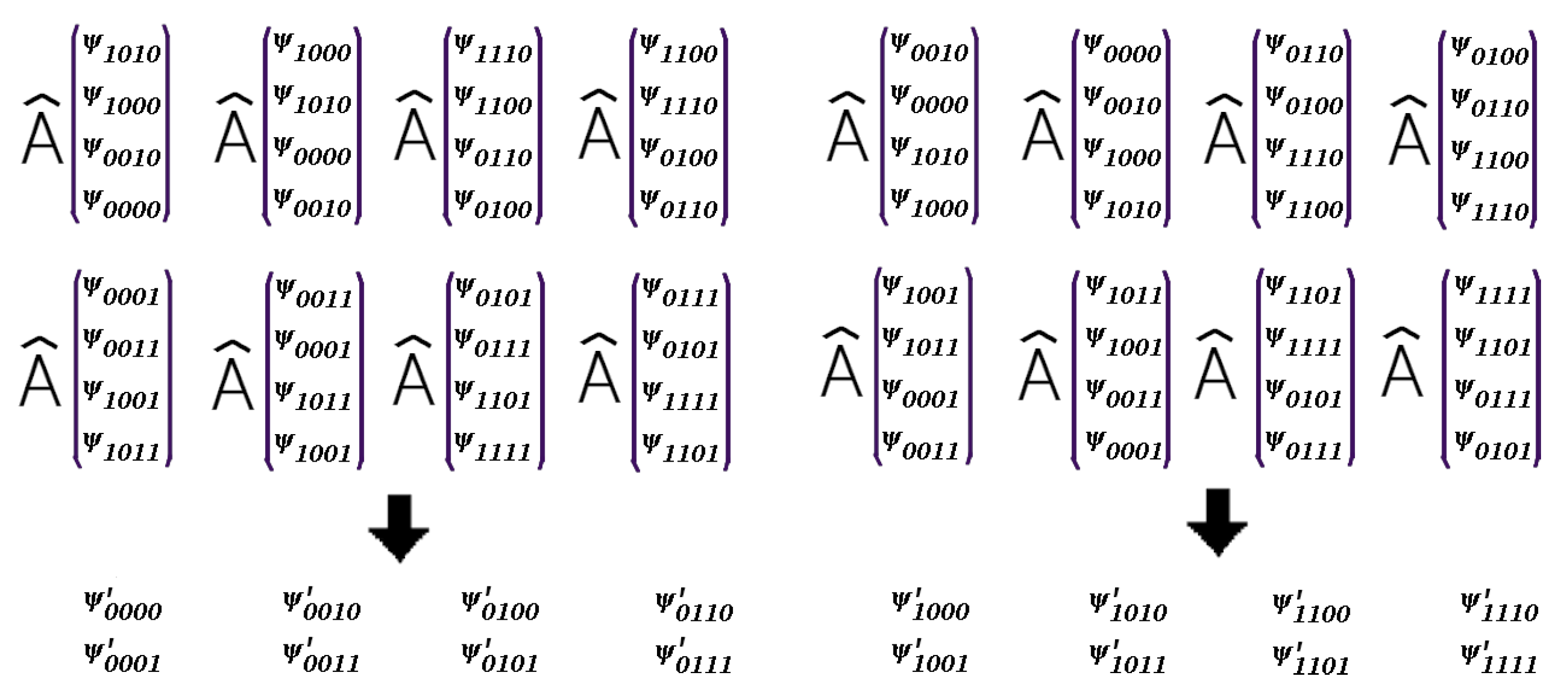
Next, we transmit the data backwards in the same way. So eventually we have $\overrightarrow{\mathsf{\Psi }}$-components in the right memory locations as it’s shown in Figure 7.

Applying $\widehat{A}$ to every one of the four components of $\overrightarrow{\mathsf{\Psi }}$ we get the result wave function. One can notice that the result component of $\overrightarrow{{\mathsf{\Psi }}^{{}^{\prime }}}$ corresponds to one of the 4 input components.

Using the given scheme, we can parallelise computations in quantum computer simulators.

5. Conclusions

In the paper the algorithm for parallel computation of two-dimensional the Edwards—Anderson model with nearest-neighbor interaction and performance data are presented. The algorithm can do a data exchange between threads so that the data of one thread can be redirected to any other thread. This follows from the diagram in Figure 4. From any thread, starting from the top line, correctly selecting the arrows and moving along them, we will definitely get to any thread we want. This allows us to use the algorithm in creating a quantum simulator. Using 64 threads it is possible to create a simulator for about 40 qubits. The computation time would roughly correspond to the data in Table 1 and Table 2, where $Lx$ would equal the number of qubits and $Ly$ would be the number of 1-qubit and 2-qubit operators. We showed that computational aspects of quantum computer simulators and Edwards-Anderson model have a lot in common. The algorithm can be used in neural networks (including the Boltzmann machine) and as a benchmark to evaluate the performance of quantum computers. Polynomial growth time of the operation time when only one side increases in size is an advantage of the method. In common case the scheme has the complexity class NP. The C++ code of the calculation program is available for downloading at [32]. It implements both minimum energy search and minimum energy configuration search.