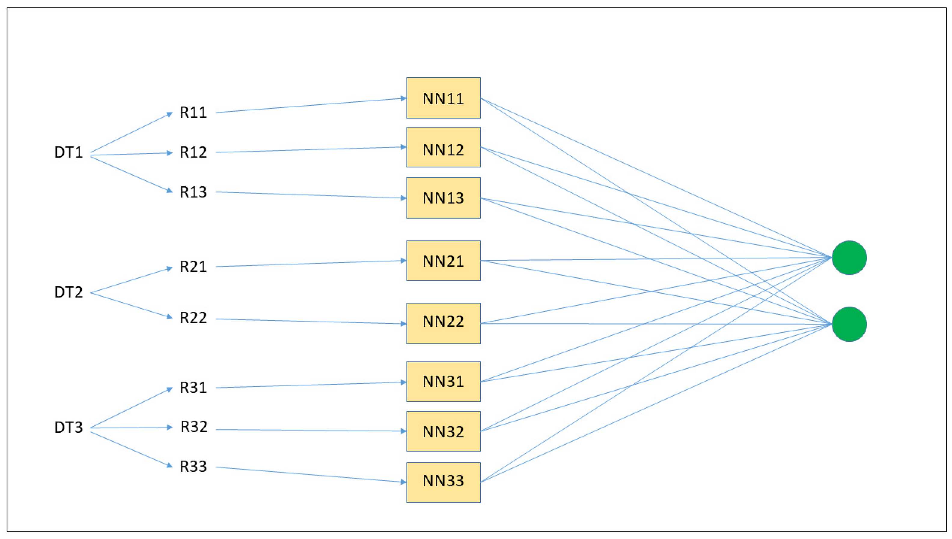
Figure 1.
Transformation of an ensemble of three DTs into an ensemble of neural networks. First, from each DT, a number of rules are generated (R11, R12, etc.); second, each rule is inserted into a single neural network (NN11, NN12, etc.); third, the final classification is the result of all of the neural networks’ classifications.
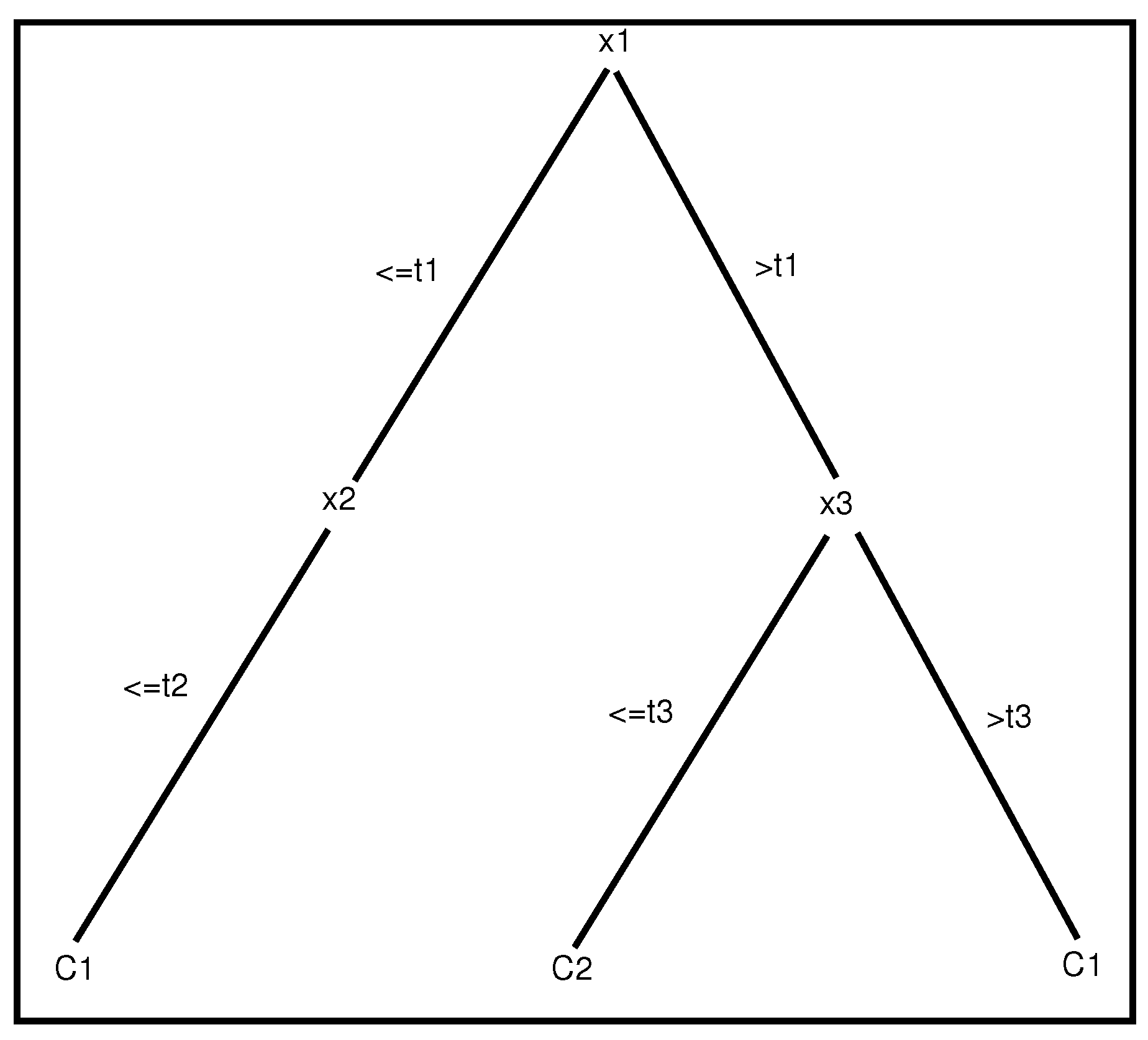
Figure 2.
An example of a tree with two depth levels. Each path from the root to a leaf represents a propositional rule of two different classes ( and ).
Figure 2.
An example of a tree with two depth levels. Each path from the root to a leaf represents a propositional rule of two different classes ( and ).
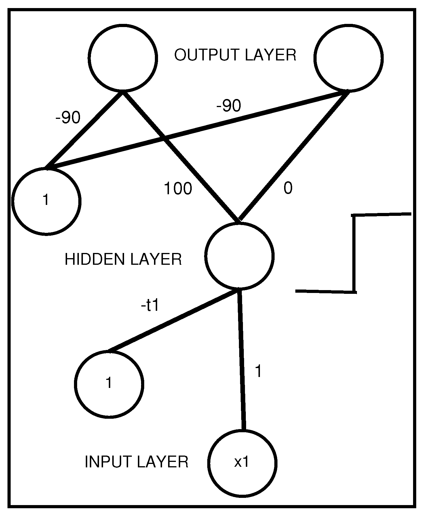
Figure 3.
An interpretable MLP coding a propositional rule with a unique antecedent .
Figure 3.
An interpretable MLP coding a propositional rule with a unique antecedent .
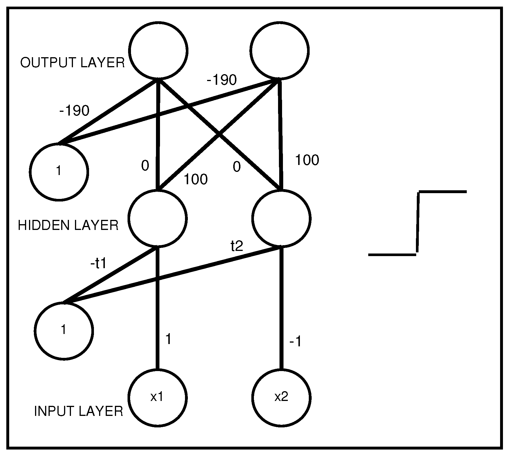
Figure 4.
An interpretable MLP coding a propositional rule with two antecedents, AND .
Figure 4.
An interpretable MLP coding a propositional rule with two antecedents, AND .
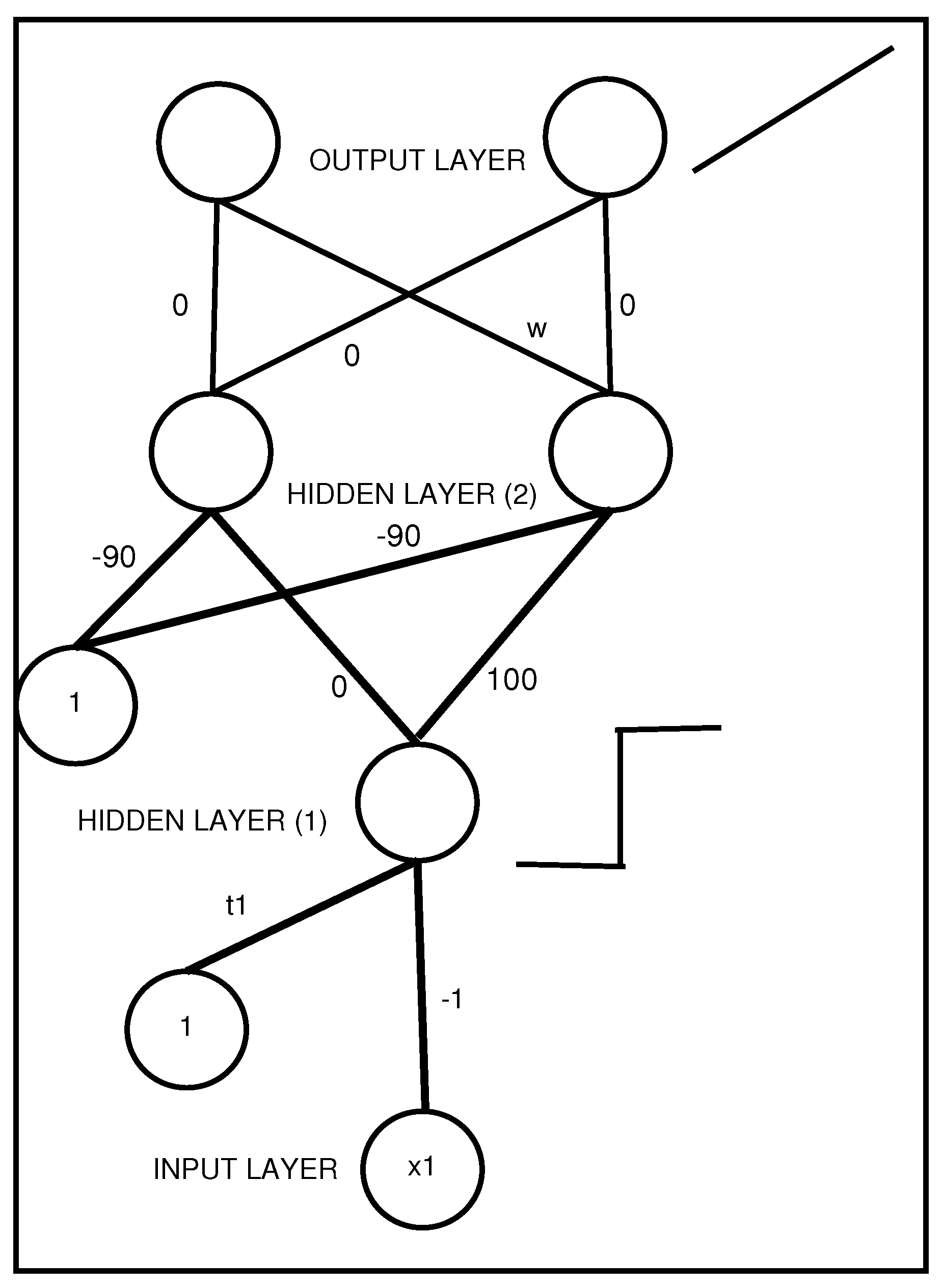
Figure 5.
An MLP with two hidden layers that represents a propositional rule with a unique antecedent . The activation function of the output layer is the identity, with coefficient w representing the rule weight.
Figure 5.
An MLP with two hidden layers that represents a propositional rule with a unique antecedent . The activation function of the output layer is the identity, with coefficient w representing the rule weight.
Table 1.
Datasets used in the experiments. From left to right, the columns designate: number of samples; number of input features; types of features (Boolean, categorical, integer, real); proportion of samples in the majority class; references.
Table 1.
Datasets used in the experiments. From left to right, the columns designate: number of samples; number of input features; types of features (Boolean, categorical, integer, real); proportion of samples in the majority class; references.
| Dataset | #Samp. | #Attr. | Attr. Types | Maj. Class (%) | Ref. |
|---|
| Australian Credit Appr. | 690 | 14 | bool., cat., int., real | 55.5 | [32] |
| Breast Cancer | 683 | 9 | int. | 65.0 | [33] |
| Divorce Prediction | 170 | 54 | bool. | 50.6 | [34] |
| Heart Disease | 270 | 13 | bool, cat., int., real | 55.6 | [31] |
| Ionosphere | 351 | 34 | int., real | 64.1 | [35] |
| Mammographic Mass | 830 | 5 | int., cat. | 51.4 | [36] |
| Student Perf. (Math) | 649 | 32 | bool., cat., int. | 67.1 | [37] |
| Voting Records | 435 | 16 | bool. | 61.4 | [38] |
Table 2.
Average results obtained on the “Australian” dataset. From left to right are presented the average results on predictive accuracy, fidelity on the testing sets, predictive accuracy of the rules, predictive accuracy of the rules when ensembles and rules agreed, number of rules, and number of antecedents per rule. Standard deviations are given between brackets. For DIMLP, RF, RF-3, and RS, the number of predictors is given between brackets (first column). For GB, the first number in brackets is the depth of the trees and the second is the number of predictors. For each column, the highest average accuracy or average fidelity is represented in bold, along with the lowest average number of rules or average number of antecedents.
| Model | Acc. | Fid. | Acc. R. (a) | Acc. R. (b) | Nb. R. | Nb. Ant. |
|---|
| DIMLP (25) | 86.8 (0.6) | 98.1 (0.4) | 86.5 (0.7) | 87.4 (0.6) | 22.2 (0.4) | 3.6 (0.1) |
| DIMLP (50) | 86.9 (0.4) | 98.2 (0.4) | 86.5 (0.6) | 87.4 (0.4) | 22.8 (0.4) | 3.7 (0.0) |
| DIMLP (100) | 86.8 (0.3) | 97.9 (0.5) | 86.4 (0.3) | 87.4 (0.2) | 22.5 (0.6) | 3.7 (0.1) |
| DIMLP (150) | 86.9 (0.3) | 98.0 (0.3) | 86.5 (0.4) | 87.4 (0.4) | 22.4 (1.0) | 3.7 (0.1) |
| RF (25) | 86.9 (0.4) | 95.1 (0.6) | 85.1 (0.6) | 87.9 (0.4) | 76.6 (0.9) | 4.6 (0.1) |
| RF (50) | 87.2 (0.6) | 95.5 (1.0) | 85.9 (0.5) | 88.3 (0.4) | 76.8 (0.8) | 4.6 (0.0) |
| RF (100) | 87.1 (0.4) | 96.0 (0.4) | 85.7 (0.7) | 87.9 (0.4) | 77.1 (0.9) | 4.7 (0.0) |
| RF (150) | 87.1 (0.4) | 95.3 (0.5) | 85.8 (0.9) | 88.3 (0.5) | 76.9 (0.9) | 4.6 (0.0) |
| RF-3 (25) | 85.9 (0.8) | 98.7 (0.3) | 85.8 (0.7) | 86.3 (0.7) | 17.2 (1.1) | 3.4 (0.1) |
| RF-3 (50) | 86.1 (0.4) | 98.5 (0.5) | 86.1 (0.5) | 86.7 (0.4) | 18.1 (1.1) | 3.5 (0.1) |
| RF-3 (100) | 86.4 (0.6) | 98.7 (0.4) | 86.1 (0.6) | 86.7 (0.6) | 17.6 (0.7) | 3.6 (0.1) |
| RF-3 (150) | 86.1 (0.4) | 98.4 (0.4) | 86.0 (0.3) | 86.6 (0.3) | 17.7 (0.6) | 3.6 (0.1) |
| GB (1,25) | 85.6 (0.2) | 100.0 (0.0) | 85.6 (0.2) | 85.6 (0.2) | 2.0 (0.0) | 1.0 (0.0) |
| GB (1,50) | 85.6 (0.2) | 100.0 (0.0) | 85.6 (0.2) | 85.6 (0.2) | 2.1 (0.3) | 1.0 (0.1) |
| GB (1,100) | 87.1 (0.4) | 99.3 (0.3) | 86.6 (0.5) | 87.2 (0.4) | 13.2 (0.7) | 2.8 (0.1) |
| GB (1,150) | 86.9 (0.5) | 98.8 (0.3) | 86.5 (0.4) | 87.2 (0.5) | 20.7 (0.7) | 3.3 (0.1) |
| GB (2,25) | 85.8 (0.4) | 99.8 (0.1) | 85.7 (0.4) | 85.8 (0.4) | 7.3 (0.4) | 2.2 (0.0) |
| GB (2,50) | 86.6 (0.3) | 99.2 (0.5) | 86.4 (0.5) | 86.8 (0.4) | 22.3 (0.8) | 3.3 (0.1) |
| GB (2,100) | 86.9 (0.5) | 97.7 (0.5) | 86.2 (0.6) | 87.4 (0.6) | 34.1 (0.8) | 3.9 (0.0) |
| GB (2,150) | 86.7 (0.5) | 97.3 (0.7) | 86.1 (0.5) | 87.4 (0.5) | 40.1 (0.7) | 4.1 (0.0) |
| GB (3,25) | 85.9 (0.5) | 99.0 (0.4) | 85.4 (0.5) | 86.0 (0.5) | 21.9 (0.4) | 3.4 (0.0) |
| GB (3,50) | 86.7 (0.3) | 97.9 (0.4) | 85.9 (0.6) | 87.1 (0.5) | 35.3 (1.1) | 4.0 (0.0) |
| GB (3,100) | 86.8 (0.5) | 96.6 (0.9) | 86.1 (0.8) | 87.8 (0.6) | 48.6 (0.5) | 4.2 (0.0) |
| GB (3,150) | 86.7 (0.8) | 96.4 (0.9) | 86.0 (0.7) | 87.7 (1.0) | 57.2 (0.7) | 4.3 (0.0) |
| SR (25) | — | — | 85.4 (0.2) | — | 13.2 (0.8) | 3.0 (0.0) |
| SR (50) | — | — | 85.5 (0.3) | — | 19.3 (0.8) | 3.0 (0.0) |
| SR (100) | — | — | 85.2 (0.5) | — | 28.3 (1.4) | 3.0 (0.0) |
| SR (150) | — | — | 85.5 (0.4) | — | 35.3 (1.3) | 3.0 (0.0) |
Table 3.
Average results obtained on the “Breast Cancer” dataset. For each column, the highest average accuracy or average fidelity is represented in bold, along with the lowest average number of rules or average number of antecedents.
Table 3.
Average results obtained on the “Breast Cancer” dataset. For each column, the highest average accuracy or average fidelity is represented in bold, along with the lowest average number of rules or average number of antecedents.
| Model | Acc. | Fid. | Acc. R. (a) | Acc. R. (b) | Nb. R. | Nb. Ant. |
|---|
| DIMLP (25) | 97.0 (0.2) | 98.7 (0.2) | 96.4 (0.4) | 97.3 (0.2) | 12.4 (0.6) | 2.7 (0.1) |
| DIMLP (50) | 97.2 (0.2) | 98.6 (0.4) | 96.3 (0.4) | 97.4 (0.2) | 12.5 (0.7) | 2.6 (0.1) |
| DIMLP (100) | 97.1 (0.1) | 98.8 (0.4) | 96.4 (0.4) | 97.3 (0.2) | 12.7 (0.3) | 2.7 (0.1) |
| DIMLP (150) | 97.2 (0.2) | 98.8 (0.4) | 96.4 (0.4) | 97.3 (0.3) | 12.7 (0.2) | 2.7 (0.1) |
| RF (25) | 97.0 (0.3) | 98.5 (0.4) | 96.7 (0.6) | 97.6 (0.3) | 24.6 (0.7) | 3.4 (0.1) |
| RF (50) | 97.1 (0.3) | 98.5 (0.4) | 96.7 (0.3) | 97.6 (0.3) | 24.3 (0.5) | 3.4 (0.0) |
| RF (100) | 97.2 (0.2) | 98.4 (0.5) | 96.6 (0.5) | 97.7 (0.2) | 24.2 (0.5) | 3.4 (0.0) |
| RF (150) | 97.4 (0.1) | 98.5 (0.2) | 96.9 (0.2) | 97.9 (0.2) | 24.3 (0.5) | 3.3 (0.0) |
| RF-3 (25) | 97.0 (0.4) | 98.9 (0.4) | 96.3 (0.4) | 97.1 (0.4) | 10.9 (0.7) | 2.6 (0.1) |
| RF-3 (50) | 97.1 (0.4) | 98.7 (0.5) | 96.4 (0.4) | 97.4 (0.3) | 11.0 (0.4) | 2.6 (0.0) |
| RF-3 (100) | 97.3 (0.2) | 98.7 (0.5) | 96.5 (0.3) | 97.5 (0.3) | 11.2 (0.4) | 2.6 (0.1) |
| RF-3 (150) | 97.3 (0.2) | 98.8 (0.3) | 96.5 (0.4) | 97.5 (0.2) | 11.1 (0.6) | 2.6 (0.0) |
| GB (1,25) | 97.3 (0.2) | 99.0 (0.3) | 96.7 (0.3) | 97.4 (0.2) | 11.2 (0.4) | 2.6 (0.0) |
| GB (1,50) | 96.8 (0.2) | 98.7 (0.2) | 96.1 (0.4) | 97.1 (0.3) | 11.8 (0.4) | 2.7 (0.0) |
| GB (1,100) | 96.7 (0.2) | 98.9 (0.5) | 96.3 (0.4) | 97.0 (0.3) | 12.0 (0.3) | 2.7 (0.1) |
| GB (1,150) | 96.8 (0.1) | 98.7 (0.3) | 96.3 (0.4) | 97.1 (0.3) | 12.0 (0.4) | 2.7 (0.1) |
| GB (2,25) | 96.7 (0.2) | 99.0 (0.5) | 96.1 (0.5) | 96.9 (0.3) | 10.8 (0.5) | 2.6 (0.0) |
| GB (2,50) | 96.7 (0.1) | 99.1 (0.2) | 96.3 (0.3) | 97.0 (0.3) | 12.2 (0.4) | 2.7 (0.1) |
| GB (2,100) | 96.9 (0.2) | 98.9 (0.2) | 96.3 (0.4) | 97.1 (0.3) | 15.3 (0.4) | 3.0 (0.0) |
| GB (2,150) | 96.8 (0.3) | 98.8 (0.3) | 96.1 (0.4) | 97.1 (0.2) | 17.8 (0.5) | 3.1 (0.1) |
| GB (3,25) | 96.4 (0.3) | 99.0 (0.3) | 96.0 (0.3) | 96.7 (0.3) | 11.4 (0.5) | 2.5 (0.1) |
| GB (3,50) | 96.7 (0.4) | 98.9 (0.2) | 96.2 (0.4) | 97.0 (0.3) | 14.8 (0.6) | 2.9 (0.1) |
| GB (3,100) | 96.9 (0.4) | 98.8 (0.3) | 96.2 (0.5) | 97.1 (0.5) | 22.6 (0.6) | 3.3 (0.0) |
| GB (3,150) | 96.9 (0.3) | 98.8 (0.3) | 96.2 (0.4) | 97.1 (0.4) | 23.5 (0.6) | 3.4 (0.0) |
| SR (25) | — | — | 94.4 (0.2) | — | 31.2 (1.7) | 2.7 (0.0) |
| SR (50) | — | — | 93.5 (0.4) | — | 49.5 (2.1) | 2.7 (0.0) |
| SR (100) | — | — | 93.0 (0.5) | — | 74.9 (2.6) | 2.8 (0.0) |
| SR (150) | — | — | 92.5 (0.4) | — | 92.5 (3.9) | 2.8 (0.0) |
Table 4.
Average results obtained on the “Divorce” dataset. For each column, the highest average accuracy or average fidelity is represented in bold, along with the lowest average number of rules or average number of antecedents.
Table 4.
Average results obtained on the “Divorce” dataset. For each column, the highest average accuracy or average fidelity is represented in bold, along with the lowest average number of rules or average number of antecedents.
| Model | Acc. | Fid. | Acc. R. (a) | Acc. R. (b) | Nb. R. | Nb. Ant. |
|---|
| DIMLP (25) | 98.1 (0.1) | 98.6 (0.7) | 96.7 (0.7) | 98.1 (0.1) | 5.5 (0.4) | 1.9 (0.1) |
| DIMLP (50) | 98.1 (0.1) | 98.2 (0.8) | 96.6 (1.0) | 98.2 (0.3) | 5.5 (0.6) | 1.9 (0.1) |
| DIMLP (100) | 98.1 (0.1) | 98.3 (0.6) | 96.5 (0.8) | 98.1 (0.1) | 5.3 (0.4) | 1.9 (0.1) |
| DIMLP (150) | 98.1 (0.1) | 98.5 (0.8) | 97.0 (0.8) | 98.3 (0.3) | 5.3 (0.4) | 1.9 (0.1) |
| RF (25) | 97.6 (0.4) | 98.7 (1.2) | 96.7 (1.3) | 97.8 (0.4) | 8.1 (0.5) | 2.3 (0.1) |
| RF (50) | 97.5 (0.2) | 98.8 (0.6) | 96.8 (0.7) | 97.7 (0.4) | 9.4 (0.7) | 2.4 (0.1) |
| RF (100) | 97.5 (1.5) | 98.7 (0.8) | 97.1 (0.5) | 98.0 (0.5) | 10.2 (0.5) | 2.4 (0.1) |
| RF (150) | 97.5 (1.5) | 98.7 (1.0) | 96.6 (1.2) | 97.7 (0.4) | 10.2 (0.6) | 2.4 (0.1) |
| RF-3 (25) | 97.7 (0.3) | 99.0 (0.9) | 96.8 (0.7) | 97.7 (0.3) | 4.6 (0.5) | 1.8 (0.1) |
| RF-3 (50) | 97.5 (0.2) | 98.7 (0.6) | 97.3 (1.1) | 98.0 (0.7) | 5.1 (0.6) | 1.8 (0.1) |
| RF-3 (100) | 97.5 (0.2) | 99.2 (0.7) | 97.1 (0.5) | 97.7 (0.3) | 4.8 (0.8) | 1.8 (0.1) |
| RF-3 (150) | 97.5 (0.2) | 99.0 (0.6) | 96.9 (0.4) | 97.7 (0.4) | 4.8 (0.5) | 1.8 (0.1) |
| GB (1,25) | 97.4 (0.3) | 99.1 (0.8) | 96.5 (0.7) | 97.4 (0.3) | 3.6 (0.1) | 1.5 (0.1) |
| GB (1,50) | 97.2 (0.3) | 99.4 (0.6) | 96.9 (0.5) | 97.4 (0.4) | 5.4 (0.2) | 2.0 (0.1) |
| GB (1,100) | 96.9 (0.3) | 98.5 (0.7) | 96.7 (0.8) | 97.6 (0.2) | 6.3 (0.3) | 2.1 (0.1) |
| GB (1,150) | 97.1 (0.4) | 98.1 (0.9) | 96.0 (0.9) | 97.5 (0.2) | 6.5 (0.4) | 2.1 (0.1) |
| GB (2,25) | 96.4 (0.8) | 99.2 (0.5) | 96.9 (0.7) | 97.0 (0.8) | 3.9 (0.2) | 1.5 (0.0) |
| GB (2,50) | 96.5 (0.6) | 99.3 (0.6) | 96.2 (0.6) | 96.6 (0.6) | 4.1 (0.3) | 1.5 (0.1) |
| GB (2,100) | 96.4 (0.9) | 99.4 (0.5) | 96.2 (0.8) | 96.6 (0.8) | 4.3 (0.4) | 1.6 (0.1) |
| GB (2,150) | 96.4 (0.9) | 99.4 (0.5) | 96.2 (0.8) | 96.6 (0.8) | 4.3 (0.4) | 1.6 (0.1) |
| GB (3,25) | 97.4 (0.8) | 99.4 (0.3) | 97.2 (0.9) | 97.6 (0.7) | 3.8 (0.0) | 1.5 (0.0) |
| GB (3,50) | 97.6 (1.1) | 99.5 (0.3) | 97.3 (1.0) | 97.7 (1.0) | 3.8 (0.0) | 1.5 (0.0) |
| GB (3,100) | 97.8 (0.8) | 98.9 (0.7) | 97.1 (0.8) | 98.0 (0.6) | 3.8 (0.0) | 1.5 (0.0) |
| GB (3,150) | 97.5 (0.8) | 98.6 (0.8) | 96.9 (1.0) | 97.9 (0.7) | 3.8 (0.0) | 1.5 (0.0) |
| SR (25) | — | — | 96.5 (0.7) | — | 13.9 (1.0) | 2.7 (0.0) |
| SR (50) | — | — | 96.1 (0.8) | — | 21.5 (1.4) | 2.6 (0.0) |
| SR (100) | — | — | 95.7 (0.8) | — | 32.6 (2.2) | 2.7 (0.0) |
| SR (150) | — | — | 94.4 (0.9) | — | 41.0 (1.8) | 2.7 (0.0) |
Table 5.
Average results obtained on the “Heart Disease” dataset. For each column, the highest average accuracy or average fidelity is represented in bold, along with the lowest average number of rules or average number of antecedents.
Table 5.
Average results obtained on the “Heart Disease” dataset. For each column, the highest average accuracy or average fidelity is represented in bold, along with the lowest average number of rules or average number of antecedents.
| Model | Acc. | Fid. | Acc. R. (a) | Acc. R. (b) | Nb. R. | Nb. Ant. |
|---|
| DIMLP (25) | 85.6 (0.6) | 95.5 (0.9) | 83.8 (1.3) | 86.3 (1.1) | 20.7 (0.4) | 3.2 (0.1) |
| DIMLP (50) | 85.8 (0.6) | 95.5 (1.0) | 84.4 (1.1) | 86.8 (0.9) | 20.4 (0.5) | 3.2 (0.0) |
| DIMLP (100) | 85.7 (0.5) | 95.7 (1.0) | 83.9 (0.6) | 86.4 (0.6) | 20.1 (0.4) | 3.2 (0.0) |
| DIMLP (150) | 85.7 (0.5) | 95.8 (1.0) | 83.5 (0.9) | 86.1 (0.7) | 20.0 (0.5) | 3.2 (0.0) |
| RF (25) | 81.9 (2.1) | 93.8 (1.6) | 81.0 (1.8) | 83.6 (1.6) | 39.0 (0.9) | 4.0 (0.0) |
| RF (50) | 82.3 (1.7) | 93.1 (2.0) | 80.5 (1.5) | 83.7 (1.1) | 40.0 (0.6) | 4.1 (0.0) |
| RF (100) | 82.7 (1.6) | 93.2 (1.7) | 81.4 (1.6) | 84.4 (1.1) | 39.7 (1.1) | 4.1 (0.0) |
| RF (150) | 83.3 (1.5) | 94.7 (1.3) | 81.9 (1.5) | 84.5 (0.9) | 39.8 (1.1) | 4.1 (0.0) |
| RF-3 (25) | 83.7 (1.3) | 95.9 (1.2) | 82.0 (1.4) | 84.2 (1.4) | 18.8 (0.6) | 3.1 (0.0) |
| RF-3 (50) | 83.7 (1.3) | 95.6 (1.3) | 82.8 (1.3) | 84.9 (1.1) | 17.6 (0.6) | 3.1 (0.0) |
| RF-3 (100) | 83.7 (0.8) | 96.0 (0.9) | 82.4 (1.1) | 84.5 (0.7) | 18.0 (0.5) | 3.1 (0.0) |
| RF-3 (150) | 84.7 (1.1) | 96.1 (1.3) | 82.8 (1.9) | 85.1 (1.1) | 18.1 (0.5) | 3.1 (0.0) |
| GB (1,25) | 84.7 (0.8) | 99.0 (0.6) | 84.0 (0.7) | 84.7 (0.8) | 11.0 (0.3) | 2.6 (0.0) |
| GB (1,50) | 84.9 (1.1) | 98.1 (0.8) | 84.3 (1.0) | 85.2 (0.9) | 15.2 (0.5) | 2.8 (0.0) |
| GB (1,100) | 84.0 (1.3) | 95.5 (1.6) | 82.0 (1.0) | 84.5 (1.3) | 20.9 (0.7) | 3.2 (0.0) |
| GB (1,150) | 83.2 (1.2) | 95.1 (1.0) | 81.7 (0.9) | 84.1 (1.0) | 21.9 (0.5) | 3.2 (0.0) |
| GB (2,25) | 81.3 (1.1) | 96.0 (1.1) | 81.3 (1.4) | 82.6 (1.0) | 17.0 (0.7) | 3.0 (0.0) |
| GB (2,50) | 81.6 (1.1) | 95.3 (1.3) | 80.6 (1.6) | 82.7 (1.1) | 22.7 (0.8) | 3.3 (0.1) |
| GB (2,100) | 81.6 (1.1) | 95.1 (1.6) | 79.9 (1.7) | 82.3 (1.3) | 27.5 (0.6) | 3.6 (0.0) |
| GB (2,150) | 80.8 (1.2) | 95.1 (1.6) | 80.0 (1.3) | 82.0 (1.0) | 30.8 (0.7) | 3.7 (0.0) |
| GB (3,25) | 80.8 (1.3) | 95.5 (1.4) | 80.3 (1.1) | 82.1 (1.4) | 22.8 (0.6) | 3.4 (0.0) |
| GB (3,50) | 80.4 (1.5) | 94.1 (0.9) | 80.0 (1.4) | 82.2 (1.3) | 28.4 (0.5) | 3.6 (0.0) |
| GB (3,100) | 79.9 (1.9) | 94.1 (1.5) | 79.7 (1.9) | 81.7 (2.1) | 34.8 (0.7) | 3.8 (0.0) |
| GB (3,150) | 79.8 (1.4) | 94.2 (1.8) | 78.8 (2.3) | 81.1 (1.8) | 37.3 (1.2) | 3.8 (0.0) |
| SR (25) | — | — | 77.1 (1.4) | — | 23.2 (0.9) | 3.0 (0.0) |
| SR (50) | — | — | 75.2 (2.1) | — | 36.3 (1.7) | 3.0 (0.0) |
| SR (100) | — | — | 71.4 (0.7) | — | 54.9 (2.0) | 3.0 (0.0) |
| SR (150) | — | — | 69.6 (1.4) | — | 69.5 (2.9) | 3.0 (0.0) |
Table 6.
Average results obtained on the “Ionosphere” dataset. For each column, the highest average accuracy or average fidelity is represented in bold, along with the lowest average number of rules or average number of antecedents.
Table 6.
Average results obtained on the “Ionosphere” dataset. For each column, the highest average accuracy or average fidelity is represented in bold, along with the lowest average number of rules or average number of antecedents.
| Model | Acc. | Fid. | Acc. R. (a) | Acc. R. (b) | Nb. R. | Nb. Ant. |
|---|
| DIMLP (25) | 93.4 (0.5) | 96.3 (0.8) | 92.1 (0.8) | 94.4 (0.4) | 18.5 (0.6) | 2.9 (0.0) |
| DIMLP (50) | 93.0 (0.6) | 95.8 (0.8) | 92.3 (1.1) | 94.5 (0.6) | 18.3 (0.6) | 2.9 (0.1) |
| DIMLP (100) | 93.0 (0.6) | 95.9 (0.7) | 92.1 (0.7) | 94.4 (0.5) | 18.8 (0.7) | 2.9 (0.0) |
| DIMLP (150) | 93.1 (0.7) | 96.1 (0.9) | 91.6 (0.8) | 94.1 (0.6) | 18.2 (0.8) | 2.9 (0.0) |
| RF (25) | 93.2 (0.7) | 95.7 (1.0) | 91.5 (0.8) | 94.3 (0.6) | 30.2 (1.2) | 3.6 (0.1) |
| RF (50) | 93.4 (0.5) | 95.2 (1.6) | 91.3 (1.4) | 94.5 (0.5) | 32.6 (1.4) | 3.8 (0.2) |
| RF (100) | 93.2 (0.4) | 95.3 (1.0) | 91.5 (1.3) | 94.4 (0.6) | 33.2 (1.2) | 4.0 (0.1) |
| RF (150) | 93.4 (0.4) | 95.9 (1.3) | 91.7 (1.1) | 94.4 (0.4) | 32.2 (0.7) | 4.0 (0.1) |
| RF-3 (25) | 91.9 (0.5) | 97.2 (0.5) | 91.6 (1.0) | 93.0 (0.5) | 13.7 (0.6) | 2.8 (0.1) |
| RF-3 (50) | 92.5 (0.8) | 97.2 (0.7) | 91.6 (0.7) | 93.3 (0.4) | 13.9 (0.4) | 2.8 (0.0) |
| RF-3 (100) | 92.9 (0.7) | 96.5 (0.9) | 91.8 (0.8) | 93.9 (0.8) | 14.2 (0.6) | 2.8 (0.1) |
| RF-3 (150) | 92.9 (0.4) | 96.8 (0.9) | 91.6 (0.9) | 93.6 (0.5) | 14.5 (0.7) | 2.8 (0.1) |
| GB (1,25) | 90.2 (0.4) | 99.6 (0.3) | 90.0 (0.5) | 90.3 (0.5) | 6.5 (0.4) | 1.9 (0.1) |
| GB (1,50) | 92.2 (0.7) | 98.6 (0.6) | 91.9 (0.8) | 92.6 (0.7) | 12.0 (0.3) | 2.5 (0.0) |
| GB (1,100) | 92.8 (0.6) | 98.2 (0.6) | 92.0 (1.0) | 93.2 (0.7) | 14.7 (0.5) | 2.7 (0.1) |
| GB (1,150) | 92.5 (0.7) | 97.4 (0.9) | 91.7 (1.2) | 93.2 (0.9) | 17.1 (0.3) | 2.9 (0.0) |
| GB (2,25) | 91.7 (0.4) | 99.0 (0.6) | 91.4 (0.5) | 92.0 (0.4) | 11.4 (0.5) | 2.5 (0.0) |
| GB (2,50) | 92.3 (0.6) | 97.9 (0.9) | 91.6 (0.8) | 92.9 (0.6) | 17.4 (0.6) | 2.9 (0.1) |
| GB (2,100) | 93.0 (0.4) | 96.6 (1.0) | 91.3 (1.1) | 93.6 (0.8) | 21.4 (1.0) | 3.2 (0.1) |
| GB (2,150) | 93.2 (0.5) | 96.3 (0.8) | 91.3 (0.8) | 93.9 (0.5) | 24.8 (0.9) | 3.4 (0.1) |
| GB (3,25) | 91.6 (0.6) | 97.3 (0.7) | 91.4 (0.8) | 92.6 (0.5) | 16.9 (0.9) | 2.7 (0.1) |
| GB (3,50) | 92.6 (0.5) | 97.0 (1.1) | 91.5 (0.8) | 93.3 (0.4) | 22.6 (0.7) | 3.1 (0.1) |
| GB (3,100) | 92.8 (1.0) | 96.5 (1.0) | 91.0 (1.1) | 93.4 (0.9) | 29.5 (1.2) | 3.5 (0.2) |
| GB (3,150) | 93.0 (0.7) | 95.8 (1.4) | 91.5 (1.4) | 94.1 (0.6) | 33.4 (0.8) | 4.0 (0.1) |
| SR (25) | — | — | 88.4 (0.8) | — | 14.1 (0.9) | 3.0 (0.0) |
| SR (50) | — | — | 87.2 (0.7) | — | 23.1 (0.9) | 3.0 (0.0) |
| SR (100) | — | — | 86.8 (1.5) | — | 40.9 (1.3) | 3.0 (0.0) |
| SR (150) | — | — | 85.6 (0.6) | — | 54.5.9 (2.1) | 3.0 (0.0) |
Table 7.
Average results obtained on the “Mammographic” dataset. For each column, the highest average accuracy or average fidelity is represented in bold, along with the lowest average number of rules or average number of antecedents.
Table 7.
Average results obtained on the “Mammographic” dataset. For each column, the highest average accuracy or average fidelity is represented in bold, along with the lowest average number of rules or average number of antecedents.
| Model | Acc. | Fid. | Acc. R. (a) | Acc. R. (b) | Nb. R. | Nb. Ant. |
|---|
| DIMLP (25) | 84.6 (0.2) | 99.4 (0.2) | 84.6 (0.2) | 84.8 (0.2) | 12.0 (0.4) | 2.6 (0.0) |
| DIMLP (50) | 84.6 (0.4) | 99.3 (0.2) | 84.6 (0.3) | 84.8 (0.3) | 12.1 (0.4) | 2.6 (0.0) |
| DIMLP (100) | 84.6 (0.3) | 99.4 (0.3) | 84.5 (0.2) | 84.7 (0.2) | 12.1 (0.4) | 2.6 (0.0) |
| DIMLP (150) | 84.6 (0.3) | 99.4 (0.2) | 84.5 (0.2) | 84.7 (0.3) | 12.0 (0.4) | 2.6 (0.0) |
| RF (25) | 79.3 (0.8) | 97.6 (0.5) | 78.7 (1.2) | 79.7 (1.0) | 93.0 (0.8) | 3.8 (0.0) |
| RF (50) | 79.1 (0.7) | 97.4 (0.6) | 78.8 (0.7) | 79.7 (0.6) | 94.6 (1.5) | 3.8 (0.0) |
| RF (100) | 79.2 (0.7) | 97.7 (0.2) | 78.8 (0.9) | 79.7 (0.8) | 95.6 (0.8) | 3.8 (0.1) |
| RF (150) | 79.0 (0.7) | 97.6 (0.4) | 78.4 (0.8) | 79.4 (0.8) | 95.6 (0.8) | 3.8 (0.2) |
| RF-3 (25) | 83.8 (0.5) | 99.8 (0.2) | 83.7 (0.5) | 83.8 (0.5) | 9.1 (0.6) | 2.4 (0.0) |
| RF-3 (50) | 84.1 (0.5) | 99.7 (0.2) | 83.9 (0.4) | 84.1 (0.4) | 9.5 (0.7) | 2.5 (0.0) |
| RF-3 (100) | 83.9 (0.4) | 99.8 (0.2) | 84.0 (0.5) | 84.1 (0.5) | 10.0 (0.6) | 2.5 (0.0) |
| RF-3 (150) | 84.0 (0.3) | 99.7 (0.2) | 84.1 (0.3) | 84.1 (0.3) | 10.4 (0.5) | 2.6 (0.0) |
| GB (1,25) | 84.1 (0.3) | 99.9 (0.1) | 84.1 (0.3) | 84.1 (0.3) | 5.4 (0.3) | 2.0 (0.0) |
| GB (1,50) | 84.2 (0.3) | 99.8 (0.1) | 84.1 (0.2) | 84.2 (0.3) | 10.5 (0.4) | 2.4 (0.0) |
| GB (1,100) | 84.0 (0.2) | 99.7 (0.1) | 84.1 (0.3) | 84.2 (0.3) | 12.7 (0.6) | 2.6 (0.0) |
| GB (1,150) | 83.8 (0.3) | 99.6 (0.2) | 83.9 (0.3) | 84.0 (0.3) | 14.2 (0.7) | 2.6 (0.0) |
| GB (2,25) | 84.3 (0.3) | 99.9 (0.1) | 84.3 (0.3) | 84.3 (0.3) | 8.8 (0.4) | 2.4 (0.0) |
| GB (2,50) | 83.7 (0.3) | 99.5 (0.2) | 83.9 (0.3) | 84.0 (0.3) | 12.9 (0.8) | 2.6 (0.0) |
| GB (2,100) | 83.1 (0.3) | 99.1 (0.1) | 83.4 (0.4) | 83.5 (0.3) | 18.1 (1.0) | 2.8 (0.0) |
| GB (2,150) | 82.7 (0.3) | 98.8 (0.1) | 82.9 (0.4) | 83.2 (0.3) | 21.2 (1.0) | 3.0 (0.0) |
| GB (3,25) | 84.1 (0.3) | 99.7 (0.3) | 84.1 (0.3) | 84.2 (0.4) | 13.0 (0.4) | 2.6 (0.0) |
| GB (3,50) | 83.3 (0.3) | 99.3 (0.3) | 83.4 (0.3) | 83.6 (0.4) | 18.9 (0.4) | 2.8 (0.0) |
| GB (3,100) | 82.6 (0.6) | 98.7 (0.3) | 82.6 (0.5) | 83.1 (0.6) | 29.2 (0.8) | 3.1 (0.0) |
| GB (3,150) | 82.3 (0.4) | 98.2 (0.4) | 82.2 (0.6) | 82.8 (0.5) | 37.9 (0.6) | 3.3 (0.0) |
| SR (25) | — | — | 81.7 (0.9) | — | 6.5 (0.4) | 3.0 (0.0) |
| SR (50) | — | — | 82.7 (0.5) | — | 9.5 (0.7) | 3.0 (0.0) |
| SR (100) | — | — | 83.1 (0.5) | — | 14.2 (1.1) | 3.0 (0.0) |
| SR (150) | — | — | 82.2 (0.7) | — | 17.3 (1.1) | 3.0 (0.0) |
Table 8.
Average results obtained on the “Students-on-Math” dataset. For each column, the highest average accuracy or average fidelity is represented in bold, along with the lowest average number of rules or average number of antecedents.
Table 8.
Average results obtained on the “Students-on-Math” dataset. For each column, the highest average accuracy or average fidelity is represented in bold, along with the lowest average number of rules or average number of antecedents.
| Model | Acc. | Fid. | Acc. R. (a) | Acc. R. (b) | Nb. R. | Nb. Ant. |
|---|
| DIMLP (25) | 92.2 (0.5) | 97.1 (0.8) | 91.8 (0.6) | 93.3 (0.5) | 18.5 (1.0) | 3.2 (0.1) |
| DIMLP (50) | 92.2 (0.3) | 97.5 (0.9) | 91.6 (0.8) | 93.0 (0.4) | 18.1 (0.9) | 3.2 (0.0) |
| DIMLP (100) | 92.1 (0.4) | 97.1 (0.7) | 91.3 (0.4) | 93.0 (0.6) | 18.1 (0.9) | 3.2 (0.1) |
| DIMLP (150) | 92.0 (0.4) | 96.7 (0.8) | 91.5 (0.7) | 93.2 (0.5) | 18.2 (0.6) | 3.2 (0.0) |
| RF (25) | 90.6 (0.8) | 94.3 (2.2) | 89.1 (1.5) | 92.2 (1.1) | 37.7 (4.4) | 4.0 (0.1) |
| RF (50) | 91.0 (0.8) | 90.7 (1.9) | 84.8 (2.2) | 91.8 (1.0) | 66.4 (9.3) | 4.8 (0.2) |
| RF (100) | 91.4 (0.4) | 89.6 (1.8) | 83.5 (1.5) | 91.9 (0.7) | 78.4 (3.6) | 5.1 (0.1) |
| RF (150) | 91.0 (0.6) | 89.3 (1.5) | 83.4 (1.4) | 91.7 (0.6) | 78.1 (3.1) | 5.1 (0.1) |
| RF-3 (25) | 86.1 (1.6) | 97.3 (0.6) | 86.8 (1.3) | 87.5 (1.4) | 18.5 (1.3) | 3.4 (0.2) |
| RF-3 (50) | 87.0 (1.4) | 97.6 (0.9) | 87.1 (1.2) | 88.0 (1.3) | 17.4 (1.3) | 3.4 (0.1) |
| RF-3 (100) | 87.3 (1.1) | 97.5 (0.7) | 87.4 (1.0) | 88.3 (1.2) | 17.2 (0.7) | 3.4 (0.1) |
| RF-3 (150) | 87.3 (0.8) | 97.1 (0.8) | 87.5 (1.3) | 88.6 (1.2) | 16.6 (0.9) | 3.3 (0.1) |
| GB (1,25) | 92.0 (0.2) | 100.0 (0.0) | 92.0 (0.2) | 92.0 (0.2) | 2.0 (0.0) | 1.0 (0.0) |
| GB (1,50) | 91.8 (0.3) | 100.0 (0.1) | 91.8 (0.2) | 91.8 (0.3) | 2.4 (0.1) | 1.1 (0.0) |
| GB (1,100) | 91.7 (0.4) | 99.2 (0.4) | 91.3 (0.5) | 91.8 (0.4) | 9.1 (0.5) | 2.3 (0.1) |
| GB (1,150) | 91.4 (0.6) | 98.3 (0.5) | 90.8 (0.5) | 91.8 (0.5) | 14.1 (0.6) | 2.7 (0.0) |
| GB (2,25) | 92.0 (0.2) | 100.0 (0.0) | 92.0 (0.2) | 92.0 (0.2) | 2.0 (0.1) | 1.0 (0.0) |
| GB (2,50) | 91.6 (0.3) | 99.3 (0.3) | 91.1 (0.4) | 91.7 (0.3) | 10.0 (0.8) | 2.3 (0.1) |
| GB (2,100) | 91.4 (0.6) | 97.6 (0.9) | 90.8 (0.7) | 92.1 (0.6) | 20.5 (0.6) | 3.2 (0.0) |
| GB (2,150) | 91.4 (0.6) | 96.6 (0.9) | 90.2 (0.9) | 92.3 (0.4) | 25.8 (0.3) | 3.5 (0.1) |
| GB (3,25) | 91.0 (0.4) | 99.1 (0.5) | 90.7 (0.6) | 91.2 (0.4) | 10.7 (0.8) | 2.5 (0.1) |
| GB (3,50) | 91.1 (0.8) | 97.6 (0.5) | 90.8 (1.1) | 92.0 (0.8) | 19.8 (0.8) | 3.2 (0.0) |
| GB (3,100) | 91.2 (0.8) | 97.0 (0.7) | 90.2 (0.9) | 92.0 (0.7) | 28.1 (0.6) | 3.6 (0.0) |
| GB (3,150) | 91.0 (0.7) | 96.2 (0.9) | 90.0 (1.0) | 92.1 (1.0) | 32.8 (3.0) | 3.8 (0.1) |
| SR (25) | — | — | 91.0 (0.4) | — | 13.9 (0.8) | 2.5 (0.0) |
| SR (50) | — | — | 90.9 (1.0) | — | 21.2 (1.3) | 2.6 (0.0) |
| SR (100) | — | — | 90.9 (0.5) | — | 29.5 (1.0) | 2.6 (0.0) |
| SR (100) | — | — | 90.7 (0.8) | — | 35.8 (1.0) | 2.6 (0.0) |
Table 9.
Average results obtained on the “Voting” dataset. For each column, the highest average accuracy or average fidelity is represented in bold, along with the lowest average number of rules or average number of antecedents.
Table 9.
Average results obtained on the “Voting” dataset. For each column, the highest average accuracy or average fidelity is represented in bold, along with the lowest average number of rules or average number of antecedents.
| Model | Acc. | Fid. | Acc. R. (a) | Acc. R. (b) | Nb. R. | Nb. Ant. |
|---|
| DIMLP (25) | 96.1 (0.6) | 98.3 (0.5) | 95.8 (0.9) | 96.7 (0.6) | 11.8 (0.4) | 2.9 (0.1) |
| DIMLP (50) | 96.2 (0.6) | 98.1 (0.4) | 95.6 (0.5) | 96.7 (0.5) | 12.0 (0.4) | 2.9 (0.0) |
| DIMLP (100) | 96.2 (0.5) | 98.3 (0.7) | 95.9 (0.6) | 96.9 (0.6) | 11.8 (0.4) | 2.9 (0.0) |
| DIMLP (150) | 96.2 (0.5) | 98.1 (0.6) | 95.7 (0.7) | 96.8 (0.5) | 11.8 (0.4) | 2.8 (0.0) |
| RF (25) | 96.3 (0.3) | 98.1 (0.5) | 95.2 (0.6) | 96.6 (0.4) | 23.1 (0.4) | 3.5 (0.1) |
| RF (50) | 96.0 (0.4) | 97.4 (0.8) | 94.6 (1.1) | 96.5 (0.5) | 24.0 (0.5) | 3.6 (0.0) |
| RF (100) | 96.1 (0.6) | 98.1 (0.7) | 94.7 (0.9) | 96.3 (0.6) | 24.0 (0.8) | 3.6 (0.0) |
| RF (150) | 96.3 (0.3) | 98.1 (0.6) | 94.5 (0.7) | 96.3 (0.3) | 24.1 (0.7) | 3.6 (0.0) |
| RF-3 (25) | 94.8 (0.6) | 99.2 (0.5) | 94.3 (0.8) | 94.9 (0.6) | 9.8 (1.3) | 2.5 (0.1) |
| RF-3 (50) | 94.9 (0.6) | 98.9 (0.4) | 94.4 (0.6) | 95.1 (0.6) | 8.6 (0.9) | 2.4 (0.1) |
| RF-3 (100) | 95.0 (0.5) | 99.1 (0.3) | 94.8 (0.6) | 95.3 (0.6) | 8.2 (0.8) | 2.3 (0.1) |
| RF-3 (150) | 95.2 (0.3) | 99.1 (0.4) | 94.8 (0.6) | 95.4 (0.6) | 7.6 (0.6) | 2.3 (0.1) |
| GB (1,25) | 95.2 (0.3) | 99.8 (0.2) | 95.0 (0.3) | 95.2 (0.3) | 3.2 (0.4) | 1.3 (0.1) |
| GB (1,50) | 95.3 (0.3) | 99.5 (0.2) | 95.0 (0.4) | 95.4 (0.4) | 6.4 (0.6) | 1.9 (0.1) |
| GB (1,100) | 95.7 (0.3) | 99.3 (0.3) | 95.5 (0.3) | 95.9 (0.3) | 9.2 (0.3) | 2.5 (0.0) |
| GB (1,150) | 95.7 (0.3) | 98.8 (0.7) | 95.8 (0.3) | 96.3 (0.5) | 10.3 (0.2) | 2.7 (0.0) |
| GB (2,25) | 95.3 (0.3) | 99.8 (0.2) | 95.2 (0.4) | 95.3 (0.3) | 4.1 (0.4) | 1.6 (0.1) |
| GB (2,50) | 95.8 (0.3) | 99.4 (0.4) | 95.6 (0.5) | 96.0 (0.3) | 9.0 (0.3) | 2.4 (0.1) |
| GB (2,100) | 96.4 (0.4) | 98.7 (0.3) | 96.1 (0.5) | 96.8 (0.4) | 14.1 (0.3) | 3.0 (0.0) |
| GB (2,150) | 96.6 (0.5) | 98.9 (0.4) | 96.2 (0.4) | 96.9 (0.4) | 16.0 (0.5) | 3.1 (0.0) |
| GB (3,25) | 95.7 (0.3) | 99.3 (0.4) | 95.4 (0.4) | 95.9 (0.4) | 10.2 (0.4) | 2.5 (0.0) |
| GB (3,50) | 96.4 (0.4) | 98.5 (0.4) | 96.2 (0.4) | 97.0 (0.4) | 13.2 (0.5) | 2.9 (0.0) |
| GB (3,100) | 96.3 (0.6) | 98.7 (0.6) | 95.8 (0.6) | 96.6 (0.7) | 19.2 (0.6) | 3.2 (0.0) |
| GB (3,150) | 95.9 (0.6) | 98.4 (0.5) | 95.3 (0.6) | 96.4 (0.6) | 22.7 (0.8) | 3.4 (0.0) |
| SR (25) | — | — | 94.9 (0.5) | — | 17.5 (0.9) | 3.0 (0.0) |
| SR (50) | — | — | 94.7 (0.5) | — | 23.9 (1.6) | 3.0 (0.0) |
| SR (100) | — | — | 94.5 (0.4) | — | 31.7 (0.9) | 3.0 (0.0) |
| SR (150) | — | — | 94.3 (0.6) | — | 37.7 (1.6) | 3.0 (0.0) |
Table 10.
Summary of the best average accuracies of rulesets produced by ensembles of DIMLPs or DTs. A comparison with SR (fourth column) was achieved through a Welch t-test; p-values are illustrated in the last column. A bold number represents a significantly better average predictive accuracy.
Table 10.
Summary of the best average accuracies of rulesets produced by ensembles of DIMLPs or DTs. A comparison with SR (fourth column) was achieved through a Welch t-test; p-values are illustrated in the last column. A bold number represents a significantly better average predictive accuracy.
| Dataset | Model | Acc. R. | Acc. R. (SR) | p-Value |
|---|
| Australian Credit Appr. | GB (1,100) | 86.6 (0.5) | 85.5 (0.3) | |
| Breast Cancer | RF (150) | 96.9 (0.2) | 94.4 (0.2) | |
| Divorce Prediction | GB (3,50) | 97.3 (1.0) | 96.5 (0.7) | |
| Heart Disease | DIMLP (50) | 84.4 (1.1) | 77.1 (1.4) | |
| Ionosphere | DIMLP (50) | 92.3 (1.1) | 88.4 (0.8) | |
| Mammographic Mass | DIMLP (25) | 84.6 (0.2) | 83.1 (0.5) | |
| Student Perf. (Math) | GB (1,25) | 92.0 (0.2) | 91.0 (0.4) | |
| Voting Records | GB (3,50) | 96.2 (0.4) | 94.9 (0.5) | |
Table 11.
Summary of the average number of rules extracted from the most accurate rulesets produced by DIMLPs or DTs. A comparison with SR was carried out with a Welch t-test, with p-values in the last column. A bold number represents a significantly lower number of rules.
Table 11.
Summary of the average number of rules extracted from the most accurate rulesets produced by DIMLPs or DTs. A comparison with SR was carried out with a Welch t-test, with p-values in the last column. A bold number represents a significantly lower number of rules.
| Dataset | Model | Nb. R. | Nb. R. (SR) | p-Value |
|---|
| Australian Credit Appr. | GB (1,100) | 13.2 (0.7) | 19.3 (0.8) | |
| Breast Cancer | RF (150) | 24.3 (0.5) | 31.2 (1.7) | |
| Divorce Prediction | GB (3,50) | 3.8 (0.0) | 13.9 (1.0) | |
| Heart Disease | DIMLP (50) | 20.4 (0.5) | 23.2 (0.9) | |
| Ionosphere | DIMLP (50) | 18.3 (0.6) | 14.1 (0.9) | |
| Mammographic Mass | DIMLP (25) | 12.0 (0.4) | 14.2 (1.1) | |
| Student Perf. (Math) | GB (1,25) | 2.0 (0.0) | 13.9 (0.8) | |
| Voting Records | GB (3,50) | 13.2 (0.5) | 17.5 (0.9) | |
Table 12.
Other results on the “Australian” dataset. A bold number represents a highest average accuracy of the rules.
Table 12.
Other results on the “Australian” dataset. A bold number represents a highest average accuracy of the rules.
| Model | Evaluation | Acc. R. | Nb. R. | Nb. Ant. |
|---|
| ET-FBT [24] | 10 × RS | 83.8 (2.1) | — | — |
| RF-FBT [24] | 10 × RS | 83.6 (2.5) | — | — |
| AFBT [24] | 10 × RS | 83.5 (2.0) | — | — |
| InTrees [25] | 100 × RS | 84.3 (—) | — | — |
| G-REX [16] | 1 × 10-fold-CV | 85.9 (—) | — | — |
| GB-DIMLP (1,100) | 10 × 10-fold-CV | 86.6 (0.5) | 13.2 (0.7) | 2.8 (0.1) |
Table 13.
Other results on the “Breast Cancer” dataset. A bold number represents a highest average accuracy of the rules.
Table 13.
Other results on the “Breast Cancer” dataset. A bold number represents a highest average accuracy of the rules.
| Model | Evaluation | Acc. R. | Nb. R. | Nb. Ant. |
|---|
| NH [22] | 1 × 10-fold-CV | 96 (2) | 44 (4) | — |
| RuleFit [22] | 1 × 10-fold-CV | 97 (2) | 38 (5) | — |
| RF-DHC [22] | 1 × 10-fold-CV | 96 (2) | 22 (9) | — |
| RF-SGL [22] | 1 × 10-fold-CV | 96 (2) | 43 (9) | — |
| RF-mSGL [22] | 1 × 10-fold-CV | 96 (3) | 20 (3) | — |
| ET-FBT [24] | 10 × RS | 94.7 (0.7) | — | — |
| RF-FBT [24] | 10 × RS | 95.6 (1.3) | — | — |
| AFBT [24] | 10 × RS | 95.5 (1.2) | — | — |
| InTrees [25] | 100 × RS | 95.2 (—) | — | — |
| G-REX [16] | 1 × 10-fold-CV | 95.5 (—) | — | — |
| RF-DIMLP (150) | 10 × 10-fold-CV | 96.9 (0.2) | 24.3 (0.5) | 3.3 (0.0) |
Table 14.
Other results on the “Ionosphere” dataset. A bold number represents a highest average accuracy of the rules.
Table 14.
Other results on the “Ionosphere” dataset. A bold number represents a highest average accuracy of the rules.
| Model | Evaluation | Acc. R. | Nb. R. | Nb. Ant. |
|---|
| NH [22] | 1 × 10-fold-CV | 89 (6) | 37 (6) | — |
| RuleFit [22] | 1 × 10-fold-CV | 93 (5) | 25 (3) | — |
| RF-DHC [22] | 1 × 10-fold-CV | 89 (5) | 28 (10) | — |
| RF-SGL [22] | 1 × 10-fold-CV | 93 (5) | 39 (8) | — |
| RF-mSGL [22] | 1 × 10-fold-CV | 91 (5) | 21 (4) | — |
| G-REX [16] | 1 × 10-fold-CV | 91.4 (—) | — | — |
| DIMLP (50) | 10 × 10-fold-CV | 92.3 (0.2) | 18.3 (0.6) | 2.9 (0.1) |
Table 15.
Other results on the “Mammographic” dataset. A bold number represents a highest average accuracy of the rules.
Table 15.
Other results on the “Mammographic” dataset. A bold number represents a highest average accuracy of the rules.
| Model | Evaluation | Acc. R. | Nb. R. | Nb. Ant. |
|---|
| ET-FBT [24] | 10 × RS | 79.3 (5.0) | — | — |
| RF-FBT [24] | 10 × RS | 82.2 (0.9) | — | — |
| AFBT [24] | 10 × RS | 83.4 (0.8) | — | — |
| DIMLP (25) | 10 × 10-fold-CV | 84.6 (0.2) | 12.0 (0.4) | 2.6 (0.0) |


