Article

Ensembling EfficientNets for the Classification and Interpretation of Histopathology Images

by
Athanasios Kallipolitis
1,*,
Kyriakos Revelos
2 and
Ilias Maglogiannis
1,*
1
Department of Digital Systems, University of Piraeus, 18534 Piraeus, Greece
2
251 Hellenic Air Force and Veterans General Hospital, 11525 Athens, Greece
*
Authors to whom correspondence should be addressed.
Algorithms 2021, 14(10), 278; https://doi.org/10.3390/a14100278
Submission received: 22 August 2021 / Revised: 13 September 2021 / Accepted: 24 September 2021 / Published: 26 September 2021
(This article belongs to the Special Issue Ensemble Algorithms and/or Explainability)

Abstract

:
The extended utilization of digitized Whole Slide Images is transforming the workflow of traditional clinical histopathology to the digital era. The ongoing transformation has demonstrated major potentials towards the exploitation of Machine Learning and Deep Learning techniques as assistive tools for specialized medical personnel. While the performance of the implemented algorithms is continually boosted by the mass production of generated Whole Slide Images and the development of state-of the-art deep convolutional architectures, ensemble models provide an additional methodology towards the improvement of the prediction accuracy. Despite the earlier belief related to deep convolutional networks being treated as black boxes, important steps for the interpretation of such predictive models have also been proposed recently. However, this trend is not fully unveiled for the ensemble models. The paper investigates the application of an explanation scheme for ensemble classifiers, while providing satisfactory classification results of histopathology breast and colon cancer images in terms of accuracy. The results can be interpreted by the hidden layers’ activation of the included subnetworks and provide more accurate results than single network implementations.

1. Introduction

Machine learning techniques with a dedicated emphasis on deep learning methodologies have been applied successfully on the field of health informatics as an assistive tool for the relief of workload that specialized medical personnel need to carry [1,2] and for educational purposes [3]. The iterative process of continuously evolving the concerned algorithms has brought to light more effective implementations that exceed the human eye discriminative capability [4,5,6] and enhance the objectivity criteria by means of visual patterns’ quantification. These improved implementations are, therefore, applied for the reliable and precise prognosis and diagnosis of pathologic cases.
The processing of traditional medical imaging material such as MRI’s, X-ray’s, Ultrasounds, Endoscopy, Thermography, Tomography, Microscopy, and Dermoscopy has been transformed to each digital version providing numerous benefits in a variety of tasks that were earlier performed manually [2,7,8,9,10,11,12,13]. The abovementioned tasks fall under the umbrella of well-known computer vision tasks, namely, semantic segmentation [14,15], generation [16], registration [17,18], image classification [15], and object detection [19]. In the last decade, the registered and documented ability of deep convolutional networks to identify visual patterns beyond the human perspective is gaining popularity in the field of digital pathology as well. Driven by the rise of digital scanners that produce whole slide images, the assessment of human tissue in histopathology images can be conducted by means of a virtual microscope. A whole slide image, containing in average 10 GB, can satisfy the needs of data hungry deep convolutional networks and alleviate issues concerning the creation, handling, and preservation of glass slides. In this framework, patches, extracted from whole slide images, are inserted as inputs in deep convolution networks in a supervised or unsupervised manner, exploiting the benefits of latest developments in the field of deep learning such as transfer learning with pretrained models and the unlabeled training via autoencoders or Generative Adversarial Networks (GANs) [20,21]. Apart from deep learning techniques, machine learning algorithms have been utilized in the field of digital pathology for content-based image retrieval and classification of histopathology images. While firstly introduced for text classification, the Bag of Words technique is utilized in [22,23] for the description of dense imagery content and its exploitation on the designated tasks. However, whole slide imaging is introduced to the scientific community with a newly breed set of challenges that needs to be addressed, mainly related to the polymorphism of the data formats, the big data management, the standardization of staining and the transparency, and explainability of predictions.
In this work, we focus on breast and colon cancer, which are distinguished as two of the most lethal cases, among different kinds of cancer that cause high rates of mortality worldwide. Breast cancer is the first leading disease in terms of incidents for women [24], whereas colon cancer is classified as second for women and third for men [25]. Utilizing automated machine learning techniques for the prognosis and diagnosis is vital for the early detection of malignancies in both cases aiming at total healing and avoidance of metastasis [26,27]. Towards this direction, researchers in the field of digital pathology have been occupied with the specific forms of cancer systematically. Although the availability of datasets is immense and reported results of the deep learning techniques are high [28], the need for explaining the connection between the input and the result is overlooked, yet compelling especially in the case of predictive models in healthcare information systems where the responsibility for high-stake decisions is heavy. “In order to build trust in intelligent systems and move towards their meaningful integration into our everyday lives, it is clear that we must build ‘transparent’ models that have the ability to explain why they predict what they predict” [29].
Ensemble classifiers existed before the rise of deep learning and were utilized in machine learning methods with a main purpose to increase the performance of the classifiers that they consist of. Starting from ancient Greece and the foundation of Democracy, the idea of ensemble classifiers derives from the human best practice of seeking for opinions of different experts before taking high risk decisions. The experts’ opinion in the domain of machine learning is represented by the prediction of a classifier. In an ensemble classifier, the input is analyzed by a set of classifiers, each implementing an algorithmic logic, resulting in a set of corresponding predictions that need to be combined in various manners in order to reach a final total prediction. Ensemble models have shown remarkable performance and the capability of correcting the faulty prediction of each included predictive model [30]. Such an example of exploiting the benefits of ensemble classifiers in the field of medical imaging can be manifested in [31], where authors employ a new weighted voting procedure on a self-supervised scheme towards the improved performance of medical X-ray and computed tomography images’ classification task. Apart from the advantage of providing a boost to the performance metrics, their simple implementation that relies on different architectural combinations provides the advantage of imposing explainability modules on top of existing architectures. In [32], the authors presented a weighted patch ensemble method that requires the modification of the ensemble classifier for the integration of the explainability scheme. In this work, the proposed methodology maintains the classification scheme without modifications. This is an important feature to consider, since the alteration of (removal or addition) layers may significantly influence the performance of the classifier. Therefore, leaving the neural network intact when integrating an explainability scheme is an important advantage. This integration is made possible as well, due to the nature of the well-known gradient weighted class activation mapping Grad-CAM technique [29] that can be applied effortlessly to the last convolutional layer of existing deep learning schemes without interfering with the functionality of the predictive model.
In this paper, we propose an ensemble classification scheme that is based on implementations of state-of-the-art deep convolutional networks, namely, EfficientNets [33]. Our contribution lies on the combination of this ensemble classifier with a Grad-CAM explanation scheme that can highlight the visual patterns which are responsible for each class prediction, while providing promising results. Furthermore, a standalone application that follows the principles of distributed computing is available for online validation and experimentation, providing its functionality (classification and explainability) as a web service. The remainder of the paper is organized as follows. In Section 2, the utilized datasets, hardware, and deep convolutional (CNN) architectures and methods are described in detail and in Section 3 the performance and explainability results are shown. In Section 4, the provided results are discussed in terms of a broader context and future work directions are indicated, whereas Section 5 concludes the paper.

2. Materials and Methods

2.1. Deep Learning Methods

The methodology of ensembling involves the combination of well-established classifiers in reaching a final decision. For the purposes of this study, deep convolutional neural networks are employed as the main ‘ingredients’ of an ensemble classifier. Starting from the newly developed group of CNNs called EfficientNets, the potential of combining state-of-the-art approaches in classifying histopathology with an emphasis on providing explainable results by means of a Grad-CAM technique is explored. Other types of deep architectures that are utilized herein are the InceptionNet, ExceptionNet, and the ResNet. When combined in an ensemble classifier and by the addition of the Grad-CAM explainability scheme, the final configuration achieves higher performance and provides plausible connections between the input and the result.

2.1.1. EfficientNets

EfficientNets are a group of deep convolutional networks that achieve and surpass state-of-the-art accuracy in different classification tasks with up to ten times better efficiency, thus the name (smaller and faster). Their main novelty lies on the latest achievement of AutoML, and, specifically, on the intelligent and controlled expansion of the three dimensions (width, depth, resolution) of a neural network by the utilization of a compound coefficient. Throughout years of research, the basic concern has been the growth of a neural network’s dimensions in such a way that accuracy is improved with the minimum of operations given certain resources’ constraints. Even when the minimum of operations is not a basic goal, increasing the dimensions of a neural network in a greedy manner does not have the expected results due to the vanishing gradients’ phenomenon. Efficient Nets address this issue by exploring the relation of the increase in each dimension and applying a grid search under a fixed resources constraint instead of arbitrarily changing these dimensions. The compound scaling method is summarized in the set of Equation (1):
d = αφ
w = βφ
r = γφ
α∙β2∙γ2 ≈ 2
α ≥ 1, β ≥ 1, γ ≥ 1
where φ is a global scaling factor that controls how many resources are available and α, β, γ determine how to allocate these resources to network depth, width, and resolution, respectively. By assigning φ = 1 and applying grid search, α, β and γ can be determined for a given convolutional architecture to achieve better accuracy. Once concluding with the definition of α, β and γ, φ can be gradually increased to augment the dimensions of the network towards better accuracy. The scaling method is applicable to any convolutional architecture that consists of a repeated pattern of layers. However, the authors of EfficientNets paper proposed a specific architecture where the main building block is the mobile inverted bottleneck convolution (MB Conv), shown in its three basic configurations in Figure 1. The base model of the EfficientNets group is Efficient Net B0 and its architecture is shown in Table 1, consisting mainly of MBConv1 and MBConv6. By utilizing MBConv blocks and increasing the value φ, Efficient Net group reaches its most complicated form B7. In the heart of these building blocks, two important innovations have found grounds to act: the depthwise separable convolution [34] that performs the functionality of a normal convolution with less resources and the squeeze and excitation unit that enables the network to perform dynamic channelwise feature recalibration [35]. Concerning depthwise separable convolution, the convolution operation is divided into two parts. First, the convolution is conducted depthwise, meaning that the convolution kernel is applied to each channel individually in order to learn channel dependent features and second, pointwise, meaning that a 1 × 1 kernel is applied to each point in order to combine the channel dependent learned features. In reference to the squeeze and excitation unit, the unit consists of two parts. Starting the squeeze part, global average pooling is applied to each channel leading to the formation of an 1 × 1 × C vector (where C are the channels), followed by a fully connected → ReLU → fully connected → sigmoid block (excitation part). In this manner, each channel is enhanced with additional information concerning the other channels and captures in between interactions. Finally, the output of the excitation part is multiplied with the original input.

2.1.2. InceptionNet, XceptionNet, ResNet

The above-mentioned building blocks and architectures are learned lessons through months of development and experience produced in the ever-evolving domain of deep learning and encapsulate notions that have been partially tested and evaluated in earlier deep learning architectures such as ResNet [36], XceptionNet, and InceptionNet [37]. These approaches achieved state-of-the-art results in computer vision tasks because they have incorporated these blocks partially. Once combined in a structured manner by means of a controlled augmentation mechanism such as in the EfficientNets, the performance is further improved.
ResNets are driven by the intuitive need for neural networks to grow deeper in order to understand and quantify more complex features and simultaneously compensate for the vanishing gradient issue. The authors discovered that, by adding the identity function between layers, the network can reach deeper architectures and cope with the vanishing gradient issue, since the layers where the gradients diminish rapidly gets bypassed. Since its publishing, the idea has spread around fast and is being utilized in different deep CNN architectures including EfficientNets.
Rather than investing in deeper architectures, the authors of InceptionNet prioritized the importance of creating wider approaches, meaning filters with multiple sizes, and leveraged their options between these two dimensions in order to capture salient patterns in the image that appears in different sizes. The initial version V1 was improved in terms of accuracy and speed by adding an auxiliary classifier during the training process, factorizing convolution operations and placing them at a wider grid. By further improvement of the initial proposal, the InceptionNet is now transformed in its fourth version. A combined approach of Resnet and Inception is proposed by the enhancement with residual blocks (Inception-ResNet). Moving a step forward, an extreme version of the InceptionNet, called XceptionNet, managed to achieve even better results, inspired by the inverse sequence of operation in the depthwise convolution (firstly proposed in Inception Net) and the removal of nonlinearity between convolutional layers.
In order to select the best performing DCNN architectures, multiple tests were performed with the two datasets and each of the above-mentioned approaches. The results verified the superiority of EfficientNets over the other approaches. Due to these preliminary tests, the ensemble scheme proposed later in this paper consists only of different ranks of EfficientNet.

2.1.3. Ensemble Classifiers

The ensemble classifiers notion lies on the founding principles of democracy as it was first established in ancient Greece. The Greeks did not need much to realize that the best decision is reached only when many opinions (the opinions of people) are heard and processed. This simple yet efficient idea has become for modern humans merely an intuitive action, since, on the verge of taking an important decision, they demand the opinion of several experts. However, if we were to leave the empirical and intuitive evidence alone, literature in the health informatics domain proves in a placid way that classifiers produce more accurate results when they are gathered together and their predictions–opinions are combined in different ways to reach a final result [38,39,40,41,42]. The manner utilized for the combination of different base classifiers is one of the basic criteria of characterizing ensemble classifiers. The basic classification of ensemble classifiers consists of the following three major categories: bagging, boosting, and stacking. Bagging is based on a parallel and independent learning procedure of base classifiers that are in turn combined as dictated by a deterministic averaging process, while boosting corresponds to a sequential adaptive learning method that adaptively modifies the distribution of the training set based on the performance accuracy of previously trained classifiers [41]. Stacking refers to a parallel learning algorithm that results in a training of a meta-model. This meta-model is responsible for the combination of base learners’ predictions. Another aspect of categorizing the different types of ensembling methods is related to the input patterns. Utilizing different classifiers, where one is trained with the original input and others with modified input versions, is common practice [42]. Another aspect categorizes ensemble classifiers in those that utilize different classifiers to solve the same task and those that break the original task into subtasks and employ a different classifier for each decomposed problem [43]. Moving further to distinguish ensemble classifiers by means of the manner between base classifiers achieves diversity. There exist randomized methods to populate an ensemble classifier by other classifiers and metrics-based techniques with a main concern to increase diversity to a certain extent that does not harm performance [44,45].

2.2. Explainability

Ensemble classifiers are widely utilized in classification tasks for the well-recognized virtue to improve performance metrics in terms of accuracy. However, when dealing with high stake predictive models such as those in healthcare applications, there are major concerns also related to the explanation of decision-making and the avoidance of erroneous ones. In our effort to construct models that can decipher the uncertainty of real-world problems, we have created black box mechanisms that produce accurate results but are not transparent and trustworthy [46]. For experts to embrace AI in the healthcare domain, the provided predictions should be retraceable and reliable. In this framework, efforts of computer vision researchers are directed towards the discovery of methods that can highlight the relationships and interactions between the visual patterns included in an input image and the final prediction. Unveiling these connections are of crucial importance [47] since humans demand that health threatening decisions are thoroughly justified.
Especially in the domain of computer vision and deep learning XAI (Explainable Artificial Intelligence), attempts to extract localization information of important visual patterns for decision-making have been widely witnessed. One way to achieve this goal is the construction of class activation maps [48]. Class activation mapping is a method which indicates the discriminative regions of an image that influenced the predictive model in reaching its final decision. Initially, it was mandatory that the predictive model should follow a certain architecture for the technique to provide plausible results, meaning that the output of the convolutional layers should be directed to a global average pooling layer and then directly to SoftMax activation function. This architecture, as discussed earlier, demands retraining of the predictive model and sacrifices complexity (added by the insertion of fully connected layers) for explainability. A generalization of this method (Grad-CAM) is proposed in [29]. In the same paper, the combination of Grad-CAMs with the guided-back propagation technique is proposed to provide a fine-grained pixel to pixel visualizations. This approach fits better to the visual characteristics of digital pathology images, where the patterns correspond to small cellular structures as opposed to larger structures. By computing the gradients for the score of each class with respect to the feature maps from the last convolutional layer and performing global average pooling on them, the importance weights for each feature map are obtained. In this fashion, the architecture of the predictive model remains intact.

2.3. System Architecture and Methodology

The system is developed with two main purposes:
  • Image classification;
  • Result explainability.
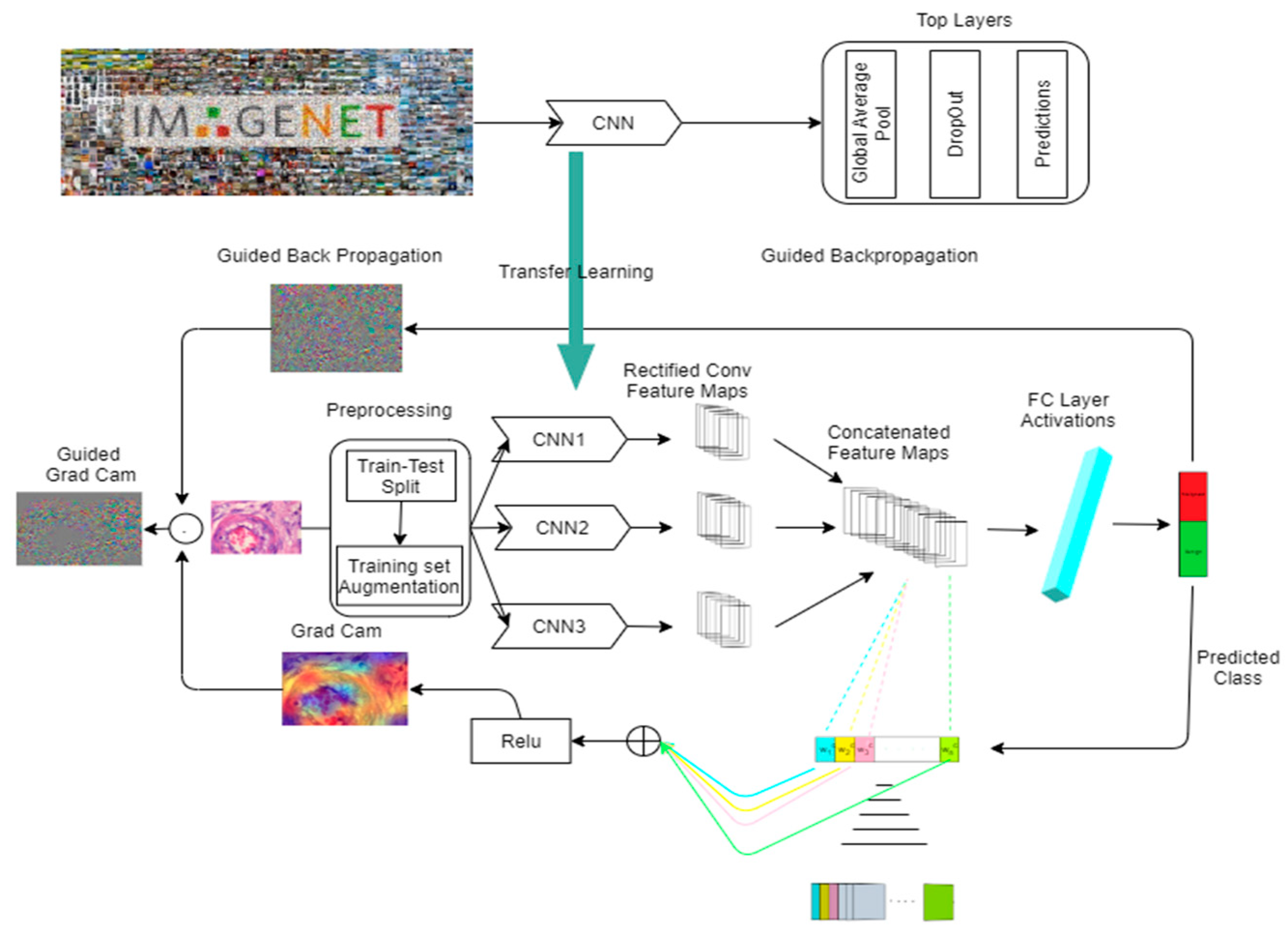
Two integrated subsystems in the whole architecture interact seamlessly and are responsible for the fulfilment of each purpose (Figure 2).
Concerning the image classification task, an ensemble classifier consisting of three different pretrained implementations of the EfficientNets group is employed in a parallel configuration that results in the concatenation of three different groups of feature maps. The pretrained models are trained by means of the ImageNet dataset [49]. The models are trained to classify 1000 general classes, thus resulting in a generalized ability to distinguish visual patterns in more specific tasks. In our method, the pretrained models are utilized without modification for feature extraction. Although fine-tuning was also performed by unfreezing a variety of top layers of the base classifiers and tuning the weights of the remaining neural network structure to the specific task, best classification results are reported with the same configuration. Prior to inserting an input image into the ensemble architecture, the images are resized and pixels normalized according to the authors’ recommended guidelines of each DCNN architecture, and the dataset is split into two parts, in 60% (training) and 40% (validation). The training set is augmented three times of the initial size by the utilization of three randomized operations, flip, rotation, and zoom. The final concatenated set of features is driven into a fully connected layer that acts as a classifier following typical best practices of deep CNNs. For the selection of the pretrained models, a preliminary examination of the individual performance on the two datasets led to the selection of the best performing models in terms of accuracy. The best individually performing deep CNNs are the Inception Net, XceptionNet, and the EfficientNets group. Consequently, an ablation study is conducted between these selections in groups of three to determine the best selection. Upon removing a CNN, the influence of this removal is measured by terms of difference in accuracy. The final selection results in the EfficientNets B1, B2, and B3. Although the basic building blocks for the three networks are the same, the required diversity in the basic classifiers of the ensemble classifier is achieved by different values provided by the compound scaling method.
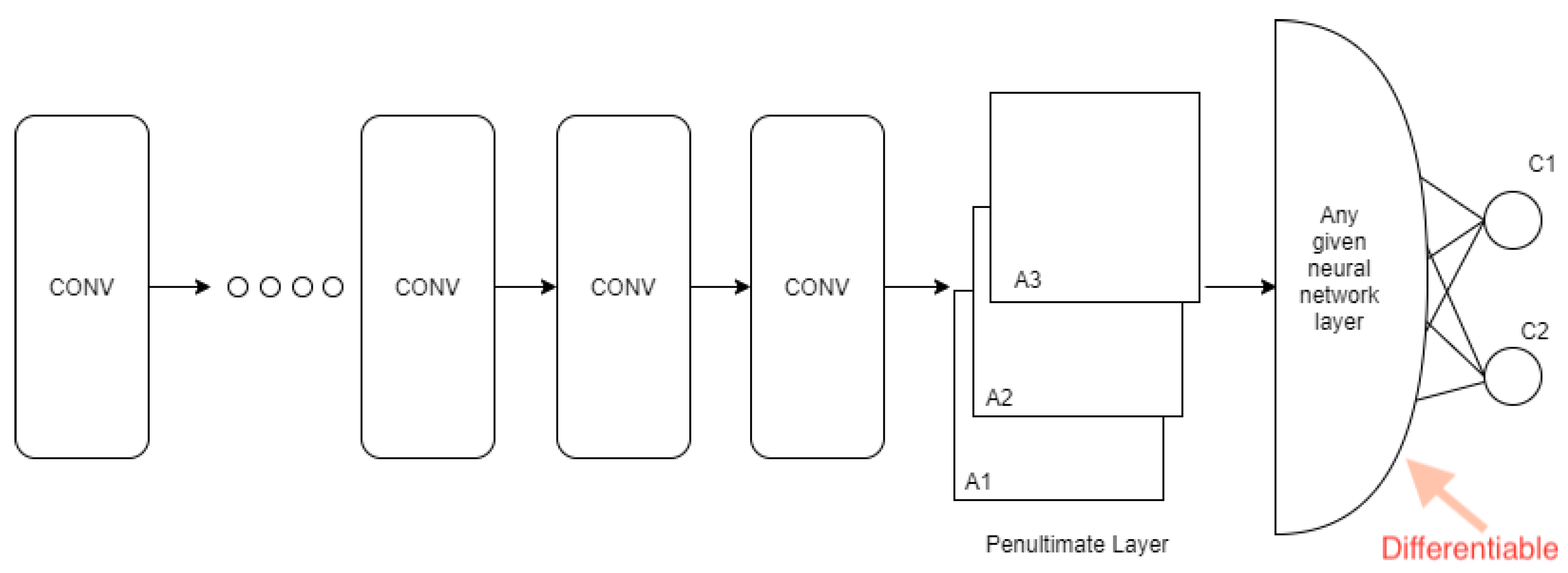
Regarding the explainability task, the concerning modules are attached to the architecture of the classification scheme while providing feedback for the localization of important visual patterns that influence the outcome of the classifier and without interfering with its functionality. When utilizing the Grad-CAM technique in a single classifier environment, the feature maps of the last convolutional layers and the gradients for the score of each class with respect to the feature maps are necessary to produce a heatmap with the explainability visualizations. As explained in [29], the technique can be divided into three steps. The first step refers to the calculation of the gradient G (Equation (2)), where Yc is the raw output of the CNN before applying softmax to turn it into a probability and Ak are the generated feature map activations. Indicator c is the class for which the heatmap is generated, since the technique is class dependent and k reflects the number of utilized convolutional filters. An important requirement for validating the results is the differentiability of the network included between the final convolutional layer and the softmax layer (Figure 3). The second step is the calculation of alpha values (Equation (3)). This operation is performed by applying global average pooling on the gradients G. Z parameter is the number of pixels in the feature map. The third step rests on the application of ReLU on the product of each feature map with the corresponding alpha value (Equation (4)):
G   = d Y c d A k
a k c = 1 Z   i = 1 v i = 1 u d Y c d A i j k
L G r a d C A M c = R e L U ( K a k c A k )
In the ensemble environment, all the necessary information regarding the calculation of the Grad-CAMs exists but needs the addition of a concatenation layer so as to bring together all extracted features’ maps. This concatenation layer takes place after the last convolutional layer of each base classifier. This minor modification enables the integration of the Grad-CAM explanation module into the ensemble classifier. Apart from the calculation of Grad-CAMs, an independent procedure is conducted in parallel, namely guided back propagation. Guided backpropagation is the combination of two distinct operations. The first is the backpropagation at ReLU activation functions. This backward pass ensures that values being greater than zero during the forward pass in the -1 filter are passed as is one step backwards. The second operation is the deconvolution at ReLU. Values being greater than zero in the current filter are passed as is one step backwards. To reach to the final heatmap, the results of guided back propagation and Grad-CAM are multiplied.

3. Experimental Results

3.1. Datasets and Hardware

Two widely utilized and publicly available datasets from the breast and colon cancer domain are the main sources of visual information that are exploited in this paper for the training and validation of the deep convolutional networks. The first dataset named Break Histological Image Classification (BreakHis) and consists of 7909 microscopic, breast tumor tissue images that are collected from 82 patients using different magnifying factors [50]. The images are:
  • Divided in 2480 benign and 5429 malignant samples;
  • 3-channel RGB (8 bits in each channel);
  • In PNG format;
  • In four different magnifying factors (40×, 100×, 200×, 400×);
  • Their dimensions are 700 × 460 pixels.
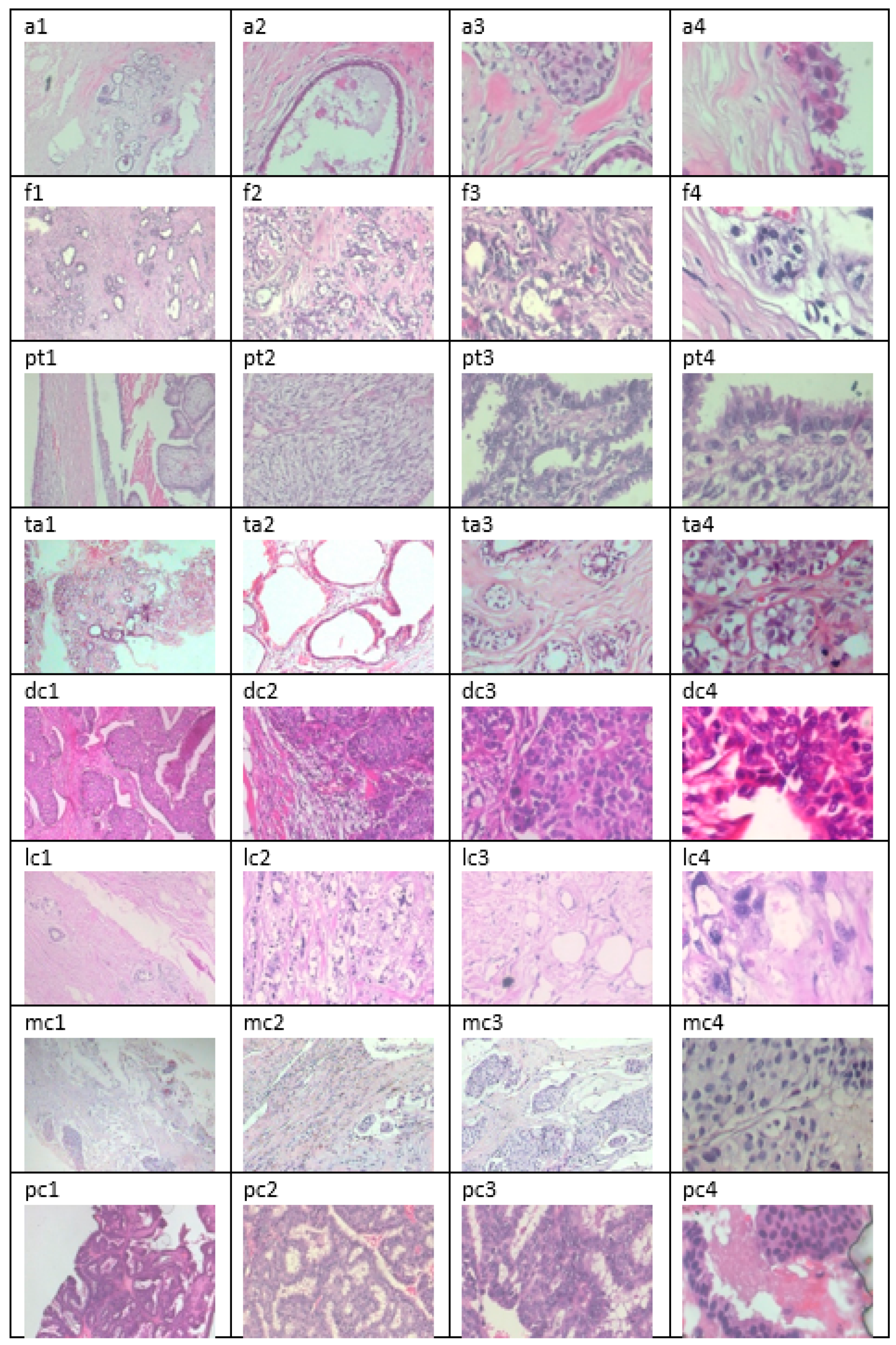
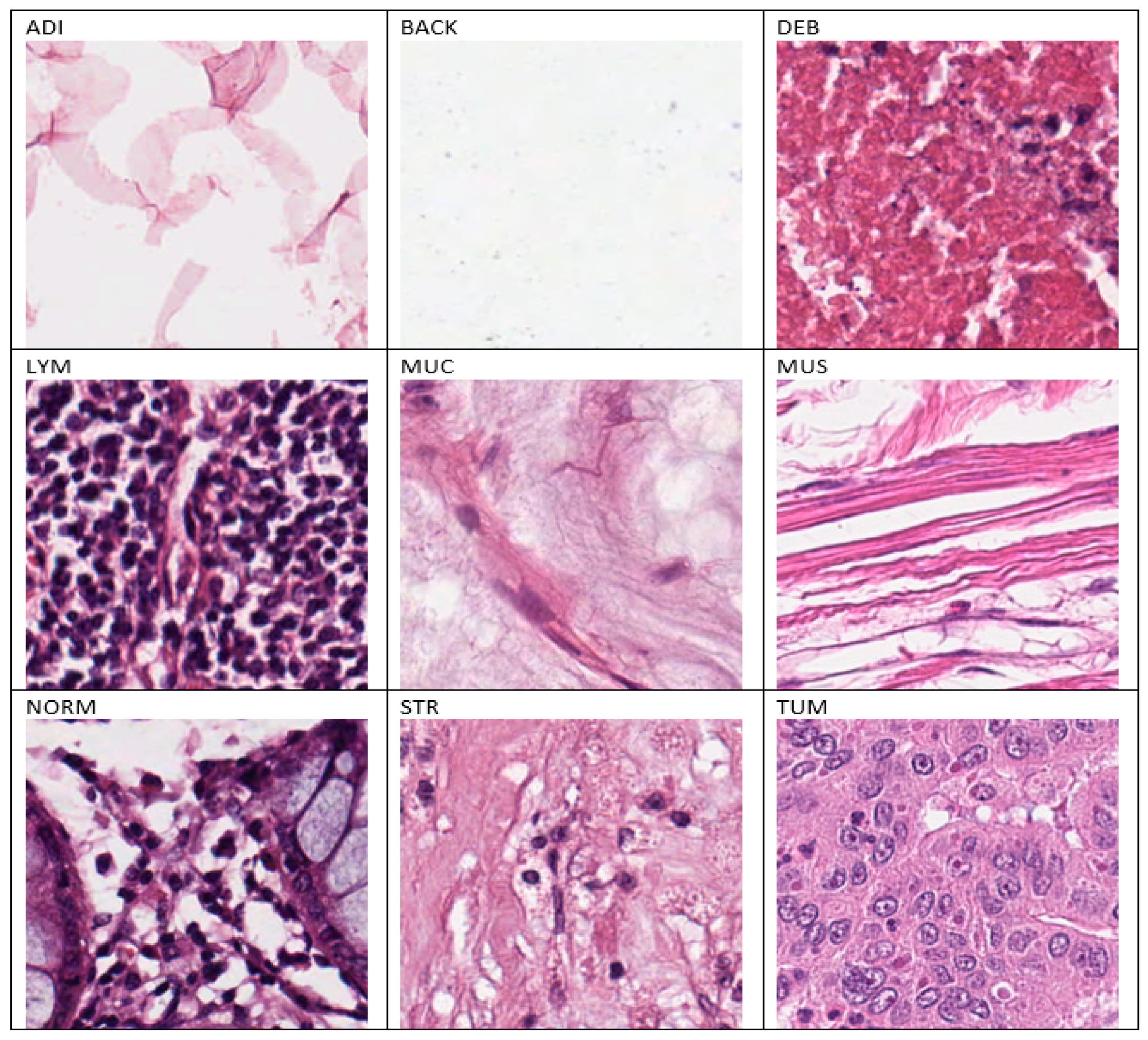
Separation of benign images in the following four distinct histological types is provided in the BreakHis dataset: adenosis (A), fibroadenoma (F), phyllodes tumor (PT), and tubular adenoma (TA). Four malignant tumor types are provided as well: ductal carcinoma (DC), lobular carcinoma (LC), mucinous carcinoma (MC), and papillary carcinoma (PC). Samples of the BreakHis dataset are shown in Figure 4 and the class distribution of the dataset is depicted in Table 2. The second dataset is a set of 100,000 non-overlapping image patches from hematoxylin & eosin (H&E) stained histological images of human colorectal cancer (CRC) and normal tissue. All images are 224 × 224 pixels at 0.5 microns per pixel (MPP). Tissue classes are: adipose (ADI), background (BACK), debris (DEB), lymphocytes (LYM), mucus (MUC), smooth muscle (MUS), normal colon mucosa (NORM), cancer-associated stroma (STR), and colorectal adenocarcinoma epithelium (TUM) [51]. Samples of the second dataset are shown in Figure 5. The class distribution of the CRC dataset is depicted in Table 3. Training and validation of the developed implementations take place on a remote configuration of a double-GPU equipped server. The GPUs are the TITAN Xp (11 GB, corecount:30 and coreClock:1.582 GHz) and the GeForce GTX 970 (4 GB, corecount:13 and coreClock: 1.392 GHz). All of the basic algorithmic operations concerning the deep neural network approaches and the Grad-CAM technique are implemented by using the TensorFlow 2.3 framework for Python programming language.

3.2. Evaluation Metrics

In terms of classification performance, the two datasets analyzed in Section 3.1 are split in 60–40% train-validation ratio for the colon cancer dataset and 70–30% for the breast cancer dataset. Although the 60–40% split in the first case is considered rather strict, this choice supports the purposes of this study concerning the trade-off between performance and explainability. Single EfficientNets achieve accuracy near perfection for the colon cancer dataset. The choice of split (60–40%) manages to lower the accuracy metric of single EfficientNets and, therefore, demonstrate the improvement in performance when utilizing ensemble classifiers. The utilized performance metrics for the binary and multiclass classification tasks are described hereafter:
  • Accuracy metric is defined as the fraction of the correctly classified instances divided by the total number of instances, as shown in Equation (5):
Accuracy = (TP + TN)/(TP + TN + FP + FN)
Correctly classified instances are analyzed in true positives (TP) and true negatives (TN), where TP are the instances predicted as positive and truly are positives (ground truth) and TN are the instances predicted as negative and truly are negative. The total number of instances consists of TP, TN, the false positive (FP), and false negative (FN) instances. FP are the instances that are predicted as positive by the classifier but are negative in reality, whereas FN are the instances predicted as negative but are positive;
  • Precision metric is defined as the fraction of the true positives divided by the true positives and false positives as shown in Equation (6):
Precision = TP/(TP + FP)
  • Recall metric is defined as the fraction of the true positives divided by the true positives and false negatives as shown in Equation (7):
Recall = TP/(TP + FN)
  • Area under Curve (AUC) metric is defined as the area under the receiver operating curve. The receiver operating curve is drawn by plotting true positive rate (TPR) versus false positive rate (FPR) at different classification thresholds. TPR is another word for recall, whereas FPR is the fraction of the false positives divided by the true negatives and false positives as shown in Equation (8):
FPR = FP/(TN + FP)
Although balanced accuracy is the appropriate performance metric when dealing with imbalanced datasets such as BreakHis, accuracy is chosen in order to provide comparison feedback in reference to the state of the art. In terms of measuring the performance of the explanation scheme, an evaluation tool runs on for specialists to test and review the results of explanation schemes. The results of this evaluation are reported in the following section.

3.3. Results

In order to determine which pretrained deep convolutional neural networks are better performing in the specific datasets, a preliminary experiment is conducted with single classifiers. We choose from the pool of the TensorFlow 2.3 API (https://www.tensorflow.org/, accessed on 23 September 2021) the following well established architectures:
  • EfficientNets B0-B7;
  • InceptionNet V3;
  • ExceptionNet;
  • VGG19;
  • ResNet152V2;
  • Inception-ResNetV2.
The hyperparameters for the deep convolutional architectures were set after experimentation to the values shown in Table 4.
To further improve the performance of each classification scheme, experiments are conducted with different custom learning rate schedulers that result in the learning rate scheduler which is expressed by Equation (9):
Lr(epochs) = Lrstart + (Lrmax − Lrstart)/(k × epoch)
where Lr defines a function that depends on epochs, Lrmax is set to 0.00005, and Lrstart to 0.0001. The difference in accuracy increases by 1.6% in the case of EfficientNet B0 when utilizing the above learning rate scheduler in contrast to using a plain Adam optimizer and k a hyperparameter that is computed by heuristic methods. In Table 5, the corresponding results for the binary (benign vs. malignant) breast cancer and for the multiclass colon cancer classification task (adipose vs. background vs. debris vs. lymphocytes vs. mucus vs. smooth muscle vs. normal colon mucosa vs. cancer associated stroma vs. colorectal adenocarcinoma epithelium) are depicted. By forming different groups of three baseline classifiers and removing one each turn, two ensemble architectures were formed. Each architecture contains the baseline implementation that had the greater impact in performance metrics when removed. The two qualified architectures are the EfficientNet group consisting of B0, B1, B2 and the group consisting of B1, B2, B3. In order to evaluate the effect of utilizing ensemble architectures against the baselines, Table 6 demonstrates the performance metrics for each configuration. The performance of the baseline architectures leaves a small space for improvement even when the dataset is split in a 60–40% ratio. Even so, the Efficient B0-2 ensemble method is on par for the colon cancer dataset.
Baseline architectures leave small space for improvement in performance; even when splitting the dataset in 60–40%, the ensemble architecture managed a minor improvement in some cases. Nevertheless, in the worst-case scenario, the proposed ensemble architectures are on par with the baseline implementations. The task of classification is made more difficult by splitting the dataset 40–60% (training–validation) and 30–70%. Each experiment is conducted by splitting the dataset into two subsets at the beginning of the study to avoid introducing bias. Consequently, each validation process is conducted without receiving any information about the images used for training. Bootstrapping the splits 10 times is performed to enhance randomness. In Table 7, the results from these two extreme splits are demonstrated. The difference in performance metrics is not significant even as the problem of classification becomes more difficult. Returning to the BreakHis dataset, four datasets are generated by the partition of the initial dataset to subsets based on the magnification factor. The four datasets correspond to the magnification factors 40×, 100×, 200×, 400×. Two classification tasks are addressed depending on the assigned labels. The first classification task is binary where the classes are benign and malignant, whereas the second classification task is multiclass where the classes are adenoma, fibroadenoma, tubular adenoma, phyllodes tumor, ductal carcinoma, lobular carcinoma, mucinous carcinoma, and papillary carcinoma. The training–validation split is set to 70–30%. As shown in Table 8 and Table 9, ensemble classifiers achieve better performance at all magnification factors in both tasks apart from one binary classification case at 100×, where classifiers perform equally.
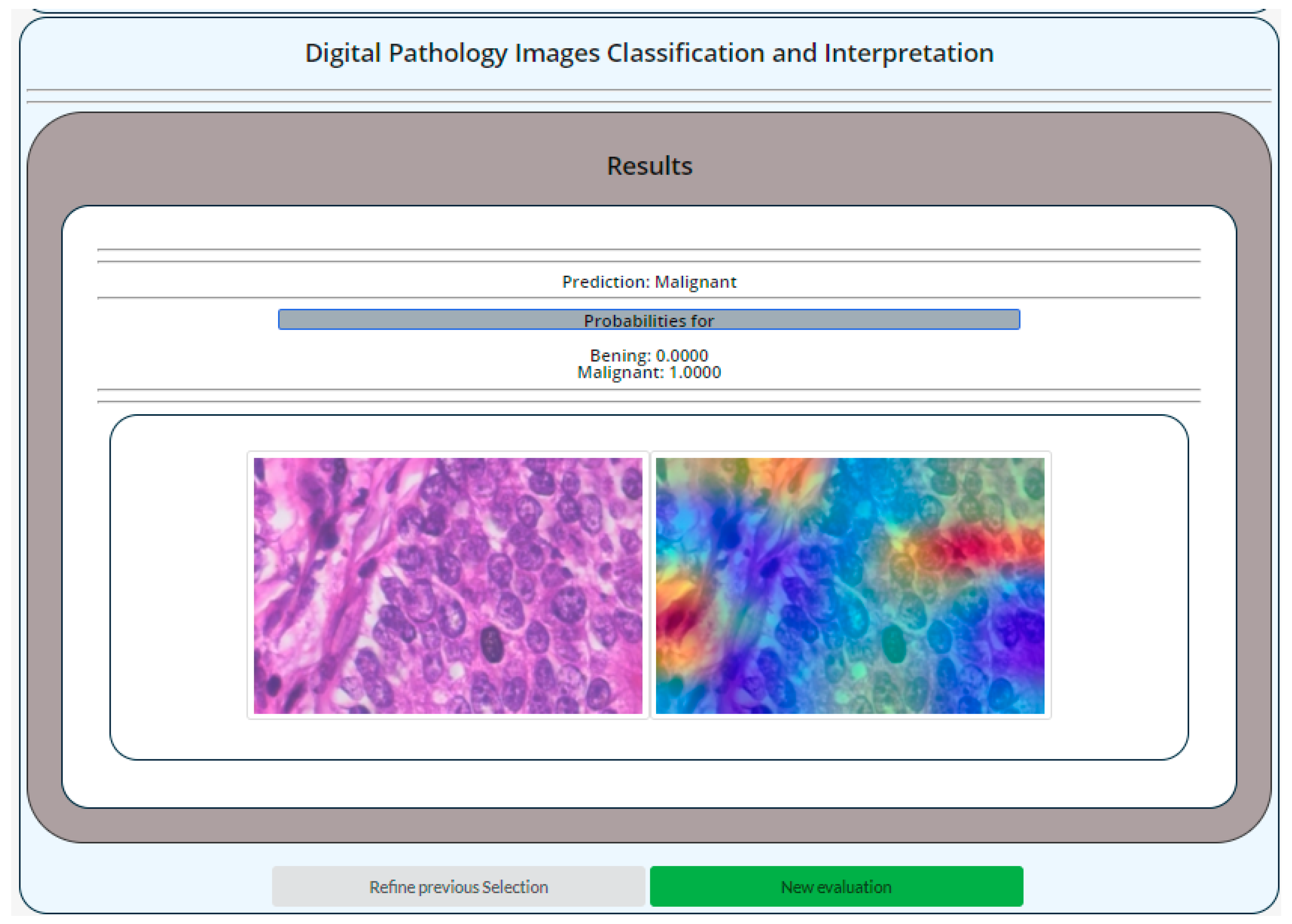
Regarding the explainability task of the proposed methodology, a test bench application was developed for visual inspection and verification of the produced results by specialized medical personnel. The web interface (Figure 6) is available in the URL http:83.212.75.102:3005/ (accessed on 23 September 2021) and upon uploading of a histopathology image, the sample is sent to the back end where the best performing ensemble architecture returns the classification result along with the generation of a heatmap of the original image. The visual patterns of the image that are characterized as highly related to the result are painted red, whereas those irrelevant with blue. The explainability capability of the different deep frameworks or ensemble classifiers are evaluated on a qualitive basis by expert pathologists in the respective field. The specialists inspect the highly related visual patterns and assess the results according to their prior experience in histopathology image-based diagnosis. The initial qualitive results show significant accordance concerning the areas responsible for the characterization of results between specialists and the ensemble classifier. The images are selected randomly from the validation set of BreakHis dataset and the Bachs dataset [52] and processed by both Grad-CAM and Guided Grad-CAM explainability techniques. The visualization and classification results are analyzed by specialized personnel and commented on terms of their opinion concerning the classification in benign or malignant class and the localization of important visual patterns that are responsible for the classification result. In Figure 7, a benign adenosis is depicted in ×400 magnification. The ensemble classifier classifies the image as probably benign but not being totally representative with high confidence in contrast to the experienced physician that refers to this image as not being totally representative of the benign class in terms of morphological patterns. The red highlighted regions are localized on epithelial tissue, though not totally. Humans tend to point their attention on the specific kind of tissue because carcinomas are malignant neoplasms of epithelial tissue. On the other hand, nearby stromal and epithelial areas are colored with yellow as they are in the vicinity of the most important regions. Concerning the Guided Grad-CAM algorithm, the coloring of respective areas is fuzzier but still more intense on the epithelial patterns.
Moving on to the next image presented in Figure 8 which is taken from the Bachs dataset and depicts an in situ carcinoma, the depicted patterns are visually representative of the malignant class. The classifier correctly predicts the class with high confidence and manages to generalize well on an unknown dataset with several variances owing to different production and staining procedures. Concerning the Grad-CAM technique, highly important regions colored as red correspond to epithelial cells, whereas, in the Guided Grad-CAM case, the coloring of respective regions is fuzzy. Some yellow painted regions are considered of less importance to the classifier and highlighted due to the vicinity to the most important regions and other yellow regions are colored with no obvious reason to experienced physicians.
In other cases, both algorithms fail to highlight the regions which are considered significant by experienced physicians. In Figure 9, drafted from the BreakHis dataset, a benign fibroadenoma is depicted. Fibroadenomas are benign tumors of the epithelial and stromal tissue. The Grad-CAM algorithm highlights mostly epithelial and stromal regions and ignores epithelial tissue on the lower left part of the image which is also indicative of the disease. Nevertheless, in terms of morphology, the depicted patterns are not highly indicative of the disease as physicians state.
A special case takes place when images contain uniform patterns of malignant or benign tissue as shown in Figure 10. In the figure, the depicted patterns are all indicative of a malignancy. Since there is no specific area of interest on the image that the algorithm individually detects as being highly responsible to the outcome, it returns medium measurements for all areas of the image, while some artifacts might be considered the cause for the assignment of high values on the edges.
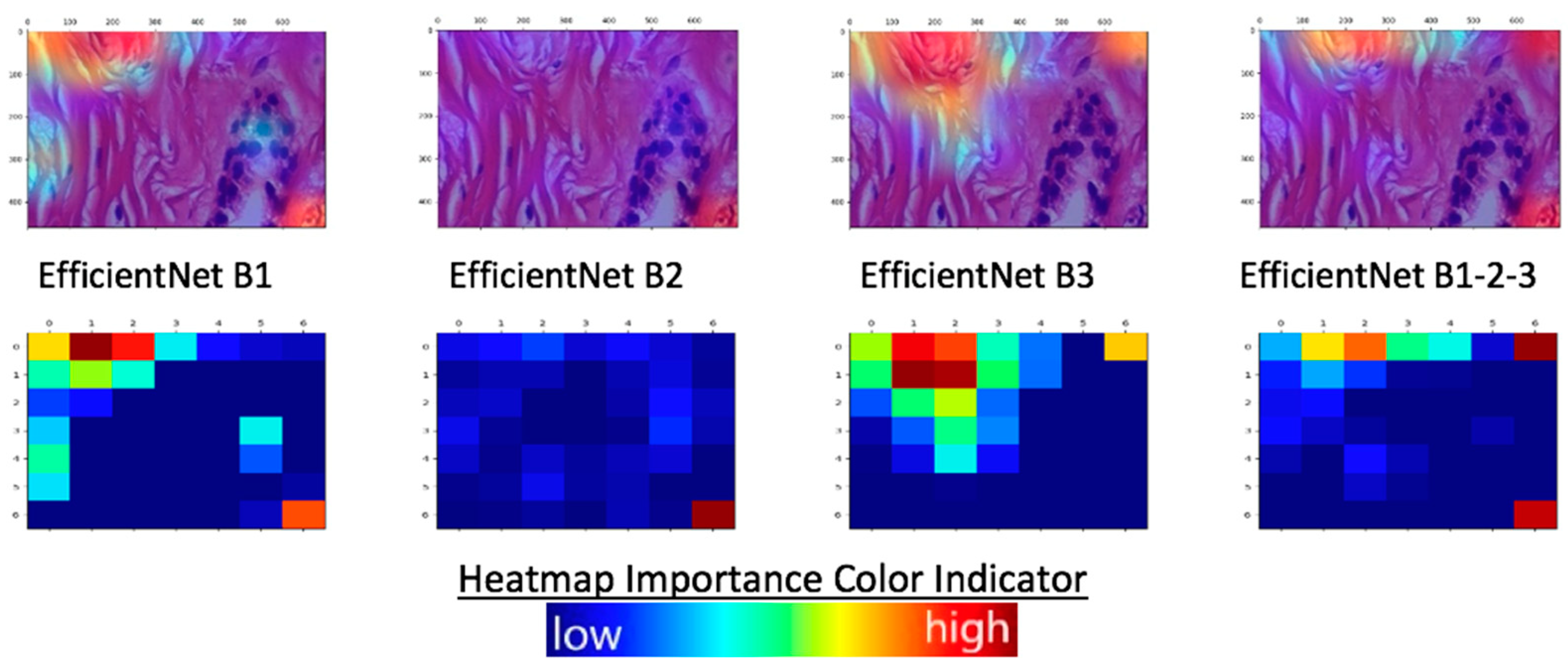
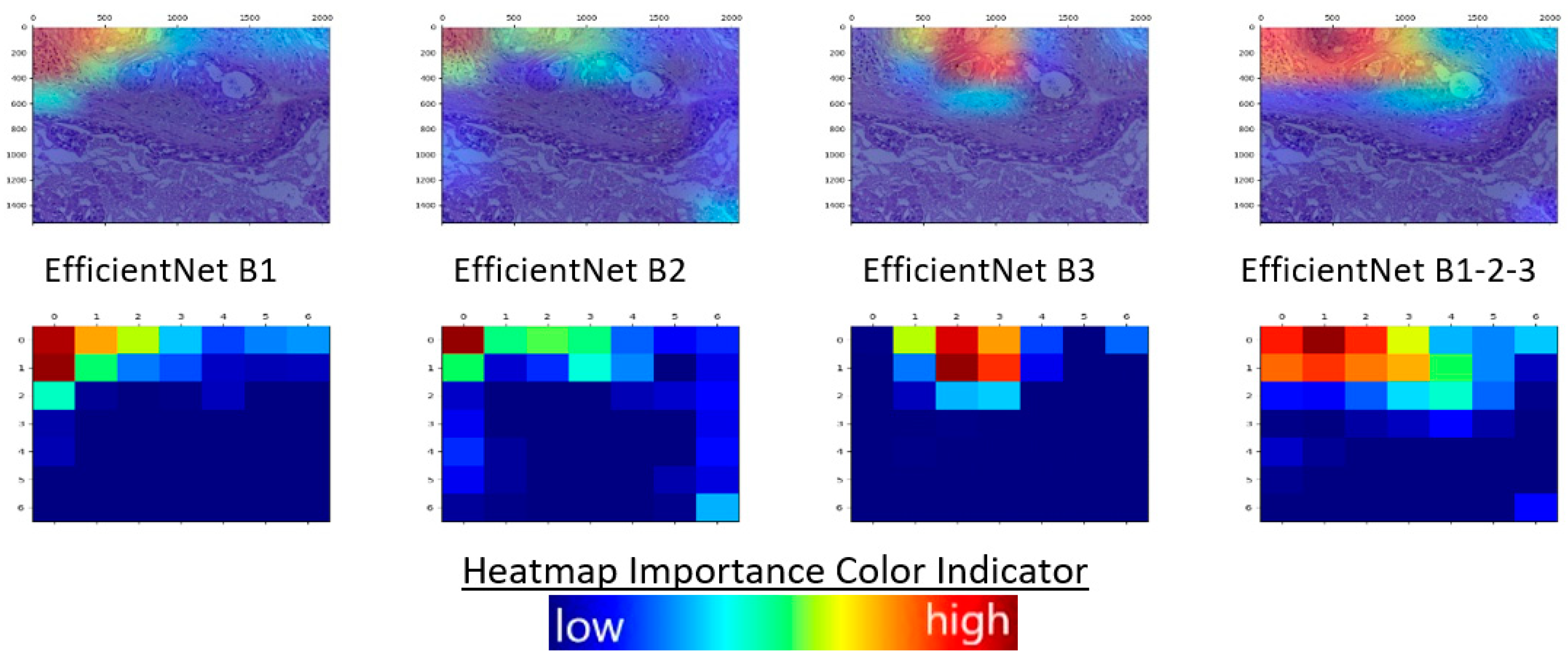
To compare the explainability properties between single and ensemble classifiers, experiments were conducted with images from the BreakHis and Bachs dataset. In Figure 11, the interpretability results of an adenosis (BreakHis) are depicted along with the respective heatmaps, whereas, in Figure 12, the corresponding outcome for an in situ carcinoma (Bachs) is shown for single and ensemble classification schemes. A closer look in results for all images and generated heatmaps concerning the base classifiers delineates that each classifier focuses on regions of interest (ROIs) that differ and/or overlay each other. To be more specific, single classifiers Efficient B1 and B2 in Figure 11 have highlighted the bottom right tile of image with high values of importance corresponding to orange and dark red colors, whereas the EfficientNet B3 classifier shows no interest on the specific tile. In the same figure, the tiles situated on the upper left corner are considered of importance to B1 and B3 classifiers, but not to B2. On the other hand, results of the ensemble classifier B1-2-3 incorporate the ROIs of the containing base classifiers on a weighted scheme in order to support the polyphony of base classifiers. This weighted aggregation of designated ROIs instead of their partial selection leads to increased accuracy performance in the case of the ensemble classifier. In Figure 11, the ensemble classifier focuses its attention on the tile situated on the lower and the upper right corner as well as the upper left area of the image by highlighting each area according to the weighted classification scheme. Taking into consideration all the tiles that base classifiers deem as important results in improved classification results. The same behavior is observed on the in situ sample in Figure 12, although the image derives from a different dataset.

4. Discussion

The main goal of the article is the proposal and evaluation of an explainability scheme in an ensemble environment and therefore the classification performance was highlighted as a secondary feature of the proposed methodology. In the proposed framework, the experimental results are produced by application of the presented methodology on two well-known datasets, BreakHis and Bachs. The utilization of different datasets enables the exploration of generalization properties.
Evaluating the classification accuracy with the utilization of images belonging to the same dataset shows that the task is trivial even for the plain architectures (not ensemble ones), the EfficientNets series supersede other well-established architectures (VGG, InceptionNet, ResNet, ExceptionNet) and achieve higher performance in both accuracy and AUC metrics for breast and colon datasets even when the training–validation split is 60–40%. The results leave small space for improvement in the case of applying the ensemble architecture. However, in some cases, such improvement occurs. The signs of better performance are more evident when splitting the datasets in a 40–60% or a 30–70% ratio. These extreme set ups make it more difficult for the plain architectures to perform as well as the ensemble configurations and, therefore, stress out the fact that the added complexity of ensemble classifiers is useful in further improving accuracy.
Utilizing ensemble architectures in order to achieve better results hinders the effort of explainability due to the added complexity. However, that is not the case for the Grad-CAM and Guided Grad-CAM technique which are seamlessly integrated in the network’s architecture. The quality of highlighting and detecting correctly the most important regions concerning the final prediction is evaluated by experienced physicians. The explainability module manages to highlight in red (highly significant) regions of the images that are indicative of the presence or absence of the respective pathology in most of the cases concerning images of the same dataset. The red highlighted regions are usually epithelial cells, and, in the case of malignancies, usually are atypical cells with hyperchromatic (dark colored) nuclei, which is in accordance with the common practice of the physicians. However, the highlighting is not performed for all similar regions in an image which would be desirable, and, in some cases, it is localized in dark colored artefacts. Therefore, the implementation of an artefact removal methodology would further enhance the generated results. Yellow colored regions (less important regions) are generated by the explainability module of the Grad-CAM technique in regions in the vicinity of red highlighted regions. A positive aspect of the method, as shown in Figure 7, as a representative sample of cases deriving from the Bachs dataset, is the fact that it generalizes well on unseen data. An important drawback of the proposed explainability methodology is the failure to highlight important regions when the morphological characteristics of the disease are uniform. To a certain extent, it is acceptable since there is no particular region that excels to highlight, and the granularity of the proposed methodology is coarse. Although the Guided Grad-CAM technique was intended to solve the issue of granularity, the provided visualizations are fuzzier than the ones presented by Grad-CAM, in contrast to the results provided by Grad-CAM that are more expressive.
Concerning the comparison of explainability properties between baseline and ensemble classifiers, it has been noted that taking into consideration all the visual patterns that baseline classifiers individually consider important can be beneficial in the same way that ensemble classifiers perform better as they combine the decisions of single classifiers on a weighted scheme.

5. Conclusions

In this work, we have investigated the application of the Grad-CAM and Guided Grad-CAM explainability techniques on ensemble classification schemes based on pretrained deep convolutional network architectures. It has been shown that the combination of different architectures improves the performance of the designated classifiers on two different use case scenarios. Concerning the explainability results, generated by the standalone web application, the initial feedback is promising in many cases but fails to distinguish important patterns where the depicted malignancy is visually uniform. Another drawback is the deficiency to localize on specific depicted morphology findings, since the Grad-CAM technique can highlight certain rectangular regions and Guided Grad-CAM is fine grained and focuses on specific pixels. Therefore, future work should be redirected towards the combination of these techniques with complementary ones that manage to distinguish morphology entities in histopathology images. In addition, future effort should be directed towards the exploration of explainability techniques that can combine the coarse-grained properties of the Grad-CAM approach with the strong discrimination abilities of the morphological patterns depicted in histopathology images.

Author Contributions

Conceptualization, A.K. and I.M.; methodology, A.K. and I.M.; software, A.K.; validation, A.K.; writing—original draft, A.K.; writing—review and editing, A.K., K.R. and I.M. All authors have read and agreed to the published version of the manuscript.

Funding

This research received no external funding.

Institutional Review Board Statement

This work did not require an approval from a research ethics board because only computational data analysis is performed, and no animal or human experimentation was involved.

Informed Consent Statement

Not applicable.

Data Availability Statement

Not applicable.

Acknowledgments

This research has been co-financed by the EU and Greek national funds through the Operational Program Competitiveness, Entrepreneurship and Innovation, under the call RESEARCH–CREATE–INNOVATE (project code: Transition—T1EDK-01385).

Conflicts of Interest

The authors declare no conflict of interest.

References

  1. Santos, M.K.; Ferreira Júnior, J.R.; Wada, D.T.; Tenório, A.; Barbosa, M.; Marques, P. Artificial intelligence, machine learning, computer-aided diagnosis, and radiomics: Advances in imaging towards to precision medicine. Radiol. Bras. 2019, 52, 387–396. [Google Scholar] [CrossRef] [Green Version]
  2. Cheng, J.Z.; Ni, D.; Chou, Y.H.; Qin, J.; Tiu, C.; Chang, Y.C.; Huang, C.S.; Shen, D.; Chen, C.M. Computer-Aided Diagnosis with Deep Learning Architecture: Applications to Breast Lesions in US Images and Pulmonary Nodules in CT Scans. Sci. Rep. 2016, 6, 24454. [Google Scholar] [CrossRef] [Green Version]
  3. Chan, K.; Zary, N. Applications and Challenges of Implementing Artificial Intelligence in Medical Education: Integrative Review. JMIR Med. Educ. 2019, 5, e13930. [Google Scholar] [CrossRef] [Green Version]
  4. Hekler, A.; Utikal, J.S.; Enk, A.H.; Solass, W.; Schmitt, M.; Klode, J.; Schadendorf, D.; Sondermann, W.; Franklin, C.; Bestvater, F.; et al. Deep learning outperformed 11 pathologists in the classification of histopathological melanoma images. Eur. J. Cancer 2019, 118, 91–96. [Google Scholar] [CrossRef] [PubMed] [Green Version]
  5. Morrow, J.M.; Sormani, M.P. Machine learning outperforms human experts in MRI pattern analysis of muscular dystrophies. Neurol. Mar. 2020, 94, 421–422. [Google Scholar] [CrossRef] [PubMed]
  6. Ardila, D.; Kiraly, A.P.; Bharadwaj, S.; Choi, B.; Reicher, J.J.; Peng, L.; Tse, D.; Etemadi, M.; Ye, W.; Corrado, G.; et al. End-to-end lung cancer screening with three-dimensional deep learning on low-dose chest computed tomography. Nat. Med. 2019, 25, 954–961. [Google Scholar] [CrossRef] [PubMed]
  7. Brosch, T.; Tam, R. Initiative for the Alzheimers Disease Neuroimaging. Manifold learning of brain MRIs by deep learning. Med. Image Comput. Comput. Assist. Interv. 2013, 16, 633–640. [Google Scholar] [CrossRef] [PubMed] [Green Version]
  8. Rajpurkar, P.; Irvin, J.; Zhu, K.; Yang, B.; Mehta, H.; Duan, T.; Ding, D.; Bagul, A.; Langlotz, C.; Shpanskaya, K.; et al. CheXNet: Radiologist-Level Pneumonia Detection on Chest X-rays with Deep Learning. arXiv 2017, arXiv:1711.05225. [Google Scholar]
  9. Cong, W.; Xi, Y.; Fitzgerald, P.; De Man, B.; Wang, G. Virtual Monoenergetic CT Imaging via Deep Learning. Patterns 2020, 1, 100128. [Google Scholar] [CrossRef] [PubMed]
  10. Soffer, S.; Klang, E.; Shimon, O.; Nachmias, N.; Eliakim, R.; Ben-Horin, S.; Kopylov, U.; Barash, Y. Deep learning for wireless capsule endoscopy: A systematic review and meta-analysis. Gastrointest. Endosc. 2020, 92, 831–839.e8. [Google Scholar] [CrossRef]
  11. Yang, J.; Wang, W.; Lin, G.; Li, Q.; Sun, Y. Infrared Thermal Imaging-Based Crack Detection Using Deep Learning. IEEE Access 2019, 7, 182060–182077. [Google Scholar] [CrossRef]
  12. Maglogiannis, I.; Delibasis, K.K. Enhancing classification accuracy utilizing globules and dots features in digital dermoscopy. Comput. Methods Programs Biomed. 2015, 118, 124–133. [Google Scholar] [CrossRef] [PubMed]
  13. Maglogiannis, I.; Sarimveis, H.; Kiranoudis, C.T.; Chatziioannou, A.A.; Oikonomou, N.; Aidinis, V. Radial basis function neural networks classification for the recognition of idiopathic pulmonary fibrosis in microscopic images. IEEE Trans. Inf. Technol. Biomed. A Publ. IEEE Eng. Med. Biol. Soc. 2008, 12, 42–54. [Google Scholar] [CrossRef] [PubMed]
  14. Prasoon, A.; Petersen, K.; Igel, C.; Lauze, F.; Dam, E.; Nielsen, M. Deep feature learning for knee cartilage segmentation using a triplanar convolutional neural network. Med. Image Comput. Comput. Assist. Interv. 2013, 16, 246–253. [Google Scholar] [CrossRef] [PubMed]
  15. Cai, L.; Gao, J.; Zhao, D. A review of the application of deep learning in medical image classification and segmentation. Ann. Transl. Med. 2020, 8, 713. [Google Scholar] [CrossRef] [PubMed]
  16. Han, C.; Hayashi, H.; Rundo, L.; Araki, R.; Shimoda, W.; Muramatsu, S.; Furukawa, Y.; Mauri, G.; Nakayama, H. GAN-based synthetic brain MR image generation. In Proceedings of the IEEE 15th International Symposium on Biomedical Imaging (ISBI 2018), Washington, DC, USA, 4–7 April 2018; pp. 734–738. [Google Scholar] [CrossRef]
  17. Haskins, G.; Kruger, U.; Yan, P. Deep learning in medical image registration: A survey. Mach. Vis. Appl. 2020, 31, 8. [Google Scholar] [CrossRef] [Green Version]
  18. Lukashevich, P.V.; Zalesky, B.A.; Ablameyko, S.V. Medical image registration based on SURF detector. Pattern Recognit. Image Anal. 2011, 21, 519. [Google Scholar] [CrossRef]
  19. Höfener, H.; Homeyer, A.; Weiss, N.; Molin, J.; Lundström, C.F.; Hahn, H.K. Deep learning nuclei detection: A simple approach can deliver state-of-the-art results. Comput. Med. Imaging Graph. 2018, 70, 43–52. [Google Scholar] [CrossRef]
  20. Kucharski, D.; Kleczek, P.; Jaworek-Korjakowska, J.; Dyduch, G.; Gorgon, M. Semi-Supervised Nests of Melanocytes Segmentation Method Using Convolutional Autoencoders. Sensors 2020, 20, 1546. [Google Scholar] [CrossRef] [Green Version]
  21. Tschuchnig, M.E.; Oostingh, G.J.; Gadermayr, M. Generative Adversarial Networks in Digital Pathology: A Survey on Trends and Future Potential. Patterns 2020, 1, 100089. [Google Scholar] [CrossRef]
  22. Kallipolitis, A.; Stratigos, A.; Zarras, A.; Maglogiannis, I. Fully Connected Visual Words for the Classification of Skin Cancer Confocal Images. In Proceedings of the 15th International Joint Conference on Computer Vision, Imaging and Computer Graphics Theory and Applications, Valletta, Malta, 27–29 February 2020; Volume 5, pp. 853–858. [Google Scholar] [CrossRef]
  23. Kallipolitis, A.; Maglogiannis, I. Creating Visual Vocabularies for the Retrieval and Classification of Histopathology Images. In Proceedings of the 41st Annual International Conference of the IEEE Engineering in Medicine and Biology Society (EMBC), Berlin, Germany, 23–27 July 2019; pp. 7036–7039. [Google Scholar] [CrossRef]
  24. López-Abente, G.; Mispireta, S.; Pollán, M. Breast and prostate cancer: An analysis of common epidemiological features in mortality trends in Spain. BMC Cancer 2014, 14, 874. [Google Scholar] [CrossRef] [PubMed] [Green Version]
  25. Forman, D.; Ferlay, J. Chapter 1.1: The Global and Regional Burden of Cancer; World Cancer Report; Stewart, B.W., Wild, C.P., Eds.; The International Agency for Research on Cancer; World Health Organization: Geneva, Switzerland, 2017; pp. 16–53. ISBN 978-92-832-0443-5. [Google Scholar]
  26. Anagnostopoulos, I.; Maglogiannis, I. Neural network-based diagnostic and prognostic estimations in breast cancer microscopic instances. Med. Biol. Eng. Comput. 2006, 44, 773–784. [Google Scholar] [CrossRef] [PubMed]
  27. Goudas, T.; Maglogiannis, I. An Advanced Image Analysis Tool for the Quantification and Characterization of Breast Cancer in Microscopy Images. J. Med. Syst. 2015, 39, 1–13. [Google Scholar] [CrossRef] [PubMed]
  28. Alinsaif, S.; Lang, J. Histological Image Classification using Deep Features and Transfer Learning. In Proceedings of the 17th Conference on Computer and Robot Vision (CRV), Ottawa, ON, Canada, 13–15 May 2020; pp. 101–108. [Google Scholar] [CrossRef]
  29. Selvaraju, R.R.; Cogswell, M.; Das, A.; Vedantam, R.; Parikh, D.; Batra, D. Grad-CAM: Visual Explanations from Deep Networks via Gradient-Based Localization. In Proceedings of the IEEE International Conference on Computer Vision (ICCV), Venice, Italy, 22–29 October 2017; pp. 618–626. [Google Scholar] [CrossRef] [Green Version]
  30. Kassani, S.H.; Kassani, P.H.; Wesolowski, M.J.; Schneider, K.A.; Deters, R. Classification of histopathological biopsy images using ensemble of deep learning networks. In Proceedings of the 29th Annual International Conference on Computer Science and Software Engineering (CASCON 19), Markham, ON, Canada, 4–6 November 2019; IBM Corp: Armonk, NY, USA, 2019; pp. 92–99. [Google Scholar]
  31. Livieris, I.E.; Kanavos, A.; Tampakas, V.; Pintelas, P. A Weighted Voting Ensemble Self-Labeled Algorithm for the Detection of Lung Abnormalities from X-Rays. Algorithms 2019, 12, 64. [Google Scholar] [CrossRef] [Green Version]
  32. Shi, X.; Xing, F.; Xu, K.; Chen, P.; Liang, Y.; Lu, Z.; Guo, Z. Loss-Based Attention for Interpreting Image-Level Prediction of Convolutional Neural Networks. IEEE Trans. Image Process. 2020, 30, 1662–1675. [Google Scholar] [CrossRef]
  33. Tan, M.; Le, Q.V. EfficientNet: Rethinking Model Scaling for Convolutional Neural Networks. arXiv 2019, arXiv:1905.11946. [Google Scholar]
  34. Chollet, F. Xception: Deep Learning with Depthwise Separable Convolutions. In Proceedings of the IEEE Conference on Computer Vision and Pattern Recognition (CVPR), Honolulu, HI, USA, 21–26 July 2017; pp. 1800–1807. [Google Scholar] [CrossRef] [Green Version]
  35. Hu, J.; Shen, L.; Sun, G.; Albanie, S. Squeeze-and-Excitation Networks. In Proceedings of the IEEE Transactions on Pattern Analysis and Machine Intelligence, Salt Lake, UT, USA, 18–23 June 2018; pp. 7132–7141. [Google Scholar]
  36. Szegedy, C.; Ioffe, S.; Vanhoucke, V.; Alemi, A. Inception-v4, Inception-ResNet and the Impact of Residual Connections on Learning. In Proceedings of the AAAI Conference on Artificial Intelligence, Phoenix, AZ, USA, 12–17 February 2016. [Google Scholar]
  37. Kaiming, H.; Xiangyu, Z.; Shaoqing, R.; Jian, S. Deep Residual Learning for Image Recognition. In Proceedings of the IEEE Conference on Computer Vision and Pattern Recognition (CVPR), Las Vegas, NV, USA, 27–30 June 2016; pp. 770–778. [Google Scholar] [CrossRef] [Green Version]
  38. Mondéjar-Guerra, V.; Novo, J.; Rouco, J.; Penedo, M.; Ortega, M. Heartbeat classification fusing temporal and morphological information of ECGs via ensemble of classifiers. Biomed. Signal Process. Control 2019, 47, 41–48. [Google Scholar] [CrossRef]
  39. Hong, S.; Wu, M.; Zhou, Y.; Wang, Q.; Shang, J.; Li, H.; Xie, J. ENCASE: An ENsemble ClASsifiEr for ECG classification using expert features and deep neural networks. In Proceedings of the Computing in Cardiology (CinC), Rennes, France, 24–27 September 2017; pp. 1–4. [Google Scholar]
  40. Gessert, N.; Nielsen, M.; Shaikh, M.; Werner, R.; Schlaefer, A. Skin lesion classification using ensembles of multi-resolution EfficientNets with meta data. MethodsX 2020, 7, 100864. [Google Scholar] [CrossRef]
  41. Livieris, I.E.; Iliadis, L.; Pintelas, P. On ensemble techniques of weight-constrained neural networks. Evol. Syst. 2021, 12, 155–167. [Google Scholar] [CrossRef]
  42. Liu, Q.; Yu, L.; Luo, L.; Dou, Q.; Heng, P. Semi-Supervised Medical Image Classification with Relation-Driven Self-Ensembling Model. IEEE Trans. Med. Imaging 2020, 39, 3429–3440. [Google Scholar] [CrossRef]
  43. Lam, L. Classifier combinations: Implementations and theoretical issues. In Proceedings of the First International Workshop on Multiple Classifier Systems of Lecture Notes in Computer Science, MCS 2000, Cagliari, Italy, 21–23 June 2000; Springer: Berlin/Heidelberg, Germany, 2000; Volume 1857, pp. 77–86. [Google Scholar]
  44. Wu, Y.; Liu, L.; Xie, Z.; Bae, J.; Chow, K.; Wei, W. Promoting High Diversity Ensemble Learning with EnsembleBench. arXiv 2020, arXiv:2010.10623. [Google Scholar]
  45. Tran, L.; Veeling, B.S.; Roth, K.; Swiatkowski, J.; Dillon, J.V.; Snoek, J.; Mandt, S.; Salimans, T.; Nowozin, S.; Jenatton, R. Hydra: Preserving Ensemble Diversity for Model Distillation. arXiv 2020, arXiv:2001.04694. [Google Scholar]
  46. Pintelas, E.; Livieris, I.E.; Pintelas, P. A Grey-Box Ensemble Model Exploiting Black-Box Accuracy and White-Box Intrinsic Interpretability. Algorithms 2020, 13, 17. [Google Scholar] [CrossRef] [Green Version]
  47. Rudin, C. Stop explaining black box machine learning models for high stakes decisions and use interpretable models instead. Nat. Mach. Intell. 2019, 1, 206–215. [Google Scholar] [CrossRef] [Green Version]
  48. Zhou, B.; Khosla, A.; Lapedriza, A.; Oliva, A.; Torralba, A. Learning Deep Features for Discriminative Localization. In Proceedings of the IEEE Conference on Computer Vision and Pattern Recognition (CVPR), Las Vegas, NV, USA, 26 June–1 July 2016; pp. 2921–2929. [Google Scholar] [CrossRef] [Green Version]
  49. Deng, J.; Dong, W.; Socher, R.; Li, L.; Li, Κ.; Li, F.-F. ImageNet: A large-scale hierarchical image database. In Proceedings of the 2009 IEEE Conference on Computer Vision and Pattern Recognition, Miami, FL, USA, 20–25 June 2009; pp. 248–255. [Google Scholar] [CrossRef] [Green Version]
  50. Spanhol, F.; Oliveira, L.S.; Petitjean, C.; Heutte, L. A Dataset for Breast Cancer Histopathological Image Classification. IEEE Trans. Biomed. Eng. 2016, 63, 1455–1462. [Google Scholar] [CrossRef] [PubMed]
  51. Kather, J.N.; Halama, N.; Marx, A. 100,000 histological images of human colorectal cancer and healthy tissue (Version v0.1). Zenodo 2018, 5281. [Google Scholar] [CrossRef]
  52. Aresta, G.; Araújo, T.; Kwok, S.; Chennamsetty, S.S.; Safwan, M.; Alex, V.; Marami, B.; Prastawa, M.; Chan, M.; Donovan, M.; et al. BACH: Grand challenge on breast cancer histology images. Med. Image Anal. 2019, 56, 122–139. [Google Scholar] [CrossRef] [PubMed]
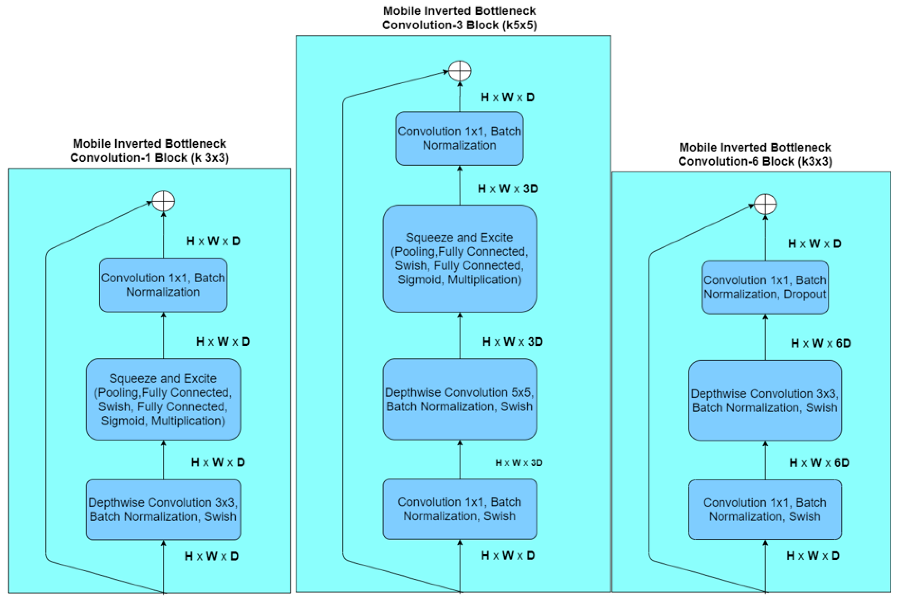
Figure 1. Three main building blocks of Efficient Nets architecture from left to right: Mobile Inverted Bottleneck Convolution-1 Block-MBlock1 (left), Mobile Inverted Bottleneck Convolution-3 Block-MBlock3 (center), Mobile Inverted Bottleneck Convolution-6 Block-MBlock6 (right).
Algorithms 14 00278 g001
Figure 2. Proposed system architecture and workflow.
Algorithms 14 00278 g002
Figure 3. Architecture of a CNN for the Grad-CAM to be applicable. The number of feature maps is set to three for visualization purposes.
Algorithms 14 00278 g003
Figure 4. This is an overview of the BreakHis dataset. Each row depicts a specific tissue type.: Adenosis is indicated as (a), fibroadenoma as (f), phyllodes tumor as (pt), and tubular adenoma as (ta), ductal carcinoma as (dc), lobular carcinoma as (lc), mucinous carcinoma as (mc), and papillary carcinoma as (pc). Each number stands for a specific magnification factor: 1 for 40×, 2 for 100×, 3 for 200×, and 4 for 400× (i.e., pc2 image depicts a papillary carcinoma in 100× magnification).
Algorithms 14 00278 g004
Figure 5. This is an overview of colon cancer dataset. Each image depicts a specific tissue type.: adipose is indicated as (ADI), background as (BACK), debris as (DEB), and lymphocytes as (LYM), mucus as (MUC), smooth muscle as (MUS), normal colon mucosa as (NORM), cancer associated stroma as (STROMA), and colorectal adenocarcinoma epithelium as (TUM).
Algorithms 14 00278 g005
Figure 6. Overview of the standalone application for the classification and explanation of histopathology images.
Algorithms 14 00278 g006
Figure 7. Application of (b) Grad-CAM and (c) Guided Grad-CAM explainability techniques on (a) a benign adenosis sample from the BreakHis dataset.
Algorithms 14 00278 g007
Figure 8. Application of (b) Grad-CAM and (c) Guided Grad-CAM explainability techniques on (a) an in situ carcinoma sample from the Bachs dataset.
Algorithms 14 00278 g008
Figure 9. Application of (b) Grad-CAM and (c) Guided Grad-CAM explainability techniques on (a) a benign fibroadenoma sample from the BreakHis dataset.
Algorithms 14 00278 g009
Figure 10. Application of (b) Grad-CAM and (c) Guided Grad-CAM explainability techniques on (a) a malignant ductal carcinoma sample from the BreakHis dataset.
Algorithms 14 00278 g010
Figure 11. Explainability results of an adenosis benign tissue sample (BreakHis dataset) for single and ensemble classifiers. The upper row depicts the outcome of the average sum between the heatmap and the original image, whereas the lower row shows the generated heatmap.
Algorithms 14 00278 g011
Figure 12. Explainability results of an in situ malignant tissue sample (BACHS dataset) for single and ensemble classifiers. The upper row depicts the outcome of the average sum between the heatmap and the original image, whereas the lower row shows the generated heatmap.
Algorithms 14 00278 g012
Table 1. Efficient Net B0 architecture.
Stage iOperator FiResolution Hi × WiChannels CiLayers Li
1Conv 3 × 3224 × 224321
2MBConv1, k3 × 3112 × 112161
3MBConv6, k3 × 3112 × 112242
4MBConv6, k5 × 556 × 56402
5MBConv6, k3 × 328 × 28 803
6MBConv6, k5 × 514 × 141123
7MBConv6, k5 × 514 × 14 1924
8MBConv6, k3 × 37 × 73201
9Conv 1 × 1, Pooling, FC7 × 712801
Table 2. Class distribution of the Breakhis dataset.
ClassSubclassesMagnification FactorsTotal
40×100×200×400×
BenignAdenosis114113111106444
Fibroadenoma2532602642371014
Tubular Adenoma109121108115453
Phyllodes Tumor149150140130569
MalignantDuctal Carcinoma8649038967883451
Lobular Carcinoma156170163137626
Mucinous Carcinoma205222196169792
Papillary Carcinoma145142135138560
Total19952081201318207909
Table 3. Class distribution of the colorectal dataset.
ClassNumber of SamplesPercentage (%)
ADI10,40710.4
BACK10,56610.56
DEB11,51311.51
LYM11,55611.56
MUC88968.9
MUS13,53713.54
STR87638.76
NORM10,44610.45
TUM14,31614.32
Table 4. Hyperparameters settings for the utilized deep CNN architectures.
HyperparametersValues
Epochs10
OptimizerAdam
Learning RateCustom
RegularizerL2
Batch size8
Table 5. Performance metrics for the breast and colon cancer dataset for baseline architectures.
Breast CancerColon Cancer
ArchitectureAccuracyAUCAccuracyAUC
EfficientNetB00.97660.99450.99460.9993
EfficientNetB10.97980.99640.98980.9984
EfficientNet B20.98170.99820.99200.9988
EfficientNet B30.98550.99880.98970.9984
EfficientNet B40.98580.99800.99100.9982
EfficientNet B50.98040.99750.99240.9982
EfficientNet B60.97280.99530.98940.9986
ExceptionNet0.97850.99420.99090.9985
InceptionNetV30.88680.94300.98440.9981
VGG160.93200.97690.97950.9969
ResNet152V20.87200.94310.95640.9913
Table 6. Performance metrics for the breast and colon cancer dataset for ensemble architectures.
Breast CancerColon Cancer
ArchitectureAccuracyAUCAccuracyAUC
EfficientNetB0-20.99250.99850.99460.9991
EfficientNetB1-30.98550.99840.98560.9989
Table 7. Performance metrics for the breast and colon cancer dataset for ensemble and plain architectures for 40–60% and 30–70% splits.
Breast CancerColon Cancer
SplitArchitectureAccuracyAUCAccuracyAUC
40–60%EfficientNetB00.97890.99740.96450.9874
EfficientNetB10.97780.99740.96880.9899
EfficientNetB20.98240.99860.97640.9906
EfficientNetB0-20.98350.99890.98220.9934
30–70%EfficientNetB00.97120.99620.96180.9822
EfficientNetB10.97370.99720.96660.9831
EfficientNetB20.97510.99680.97030.9852
EfficientNetB0-20.97850.99790.97820.9925
Table 8. Performance metrics [Accuracy (Acc), Precision (Pr), and Recall (Rec)] for the breast dataset for selected baseline and ensemble architectures at different magnification factors (40×, 100×, 200×, 400×) concerning the binary classification task.
Breast Cancer
MetricsAccPrRecAccPrRecAccPrRecAccPrRec
Magnification Factor40×100×200×400×
Architecture
EfficientNetB00.96990.96990.96990.97920.97920.97920.96310.96310.96310.95600.95600.9560
EfficientNetB10.97490.97490.97490.96790.96790.96790.94730.94730.94730.91580.91580.9158
EfficientNet B20.97990.97990.97990.97120.97120.97120.96310.96310.96310.93960.93960.9396
EfficientNet B30.97660.97660.97660.97440.97440.9744096660.96660.96660.94510.94510.9451
EfficientNetB0-20.98830.98830.98830.97120.97120.97120.97190.97190.97190.94690.94690.9469
EfficientNetB1-30.98660.98660.98660.98240.98240.98240.98590.98590.98590.96970.96970.9697
Table 9. Performance metrics [Accuracy(Acc), Precision (Pr) and Recall(Rec)] for the breast dataset for selected baseline and ensemble architectures at different magnification factors (40×, 100×, 200×, 400×) concerning the multiclass classification task.
Breast Cancer
MetricsAccPrRecAccPrRecAccPrRecAccPrRec
Magnification Factor40×100×200×400×
Architecture
EfficientNetB00.90970.92150.90300.87020.88490.86220.83130.85690.82070.83330.85520.8114
EfficientNetB10.87960.89480.86790.86380.86960.84460.83130.85690.82070.82050.83400.8004
EfficientNet B20.87960.89480.89790.87980.89180.87180.86290.87230.84010.80400.82750.7729
EfficientNet B30.89630.91030.88290.88460.88930.87500.85940.87030.84890.84430.86810.8351
EfficientNetB0-20.91140.92480.90470.86860.87440.85900.86290.89150.85240.84430.86410.8150
EfficientNetB1-30.92640.93680.91640.89630.91030.88290.86640.87750.84360.85710.87160.8333
Publisher’s Note: MDPI stays neutral with regard to jurisdictional claims in published maps and institutional affiliations.