
Overview of Algorithms for Using Particle Morphology in Pre-Detonation Nuclear Forensics


Abstract
:1. Introduction
2. CCR Results
3. Multivariate t-Test
4. LDA
5. ABC
- (1)
- Sample from the prior
- (2)
- Simulate data from the model
- (3)
- If the distance , then accept as an observation from
- (A)
- ABC allows for comparison of the performance of candidate summary statistics such as the mean or quantiles of the particle attributes such as size and shape.
- (B)
- ABC allows for easy experimentation with the effects of EDA to choose a model and to include uncertainty in the estimated forward model (such as the number of mixture components in each of ADU, AUC, SDU, MDU) used to perform ABC.
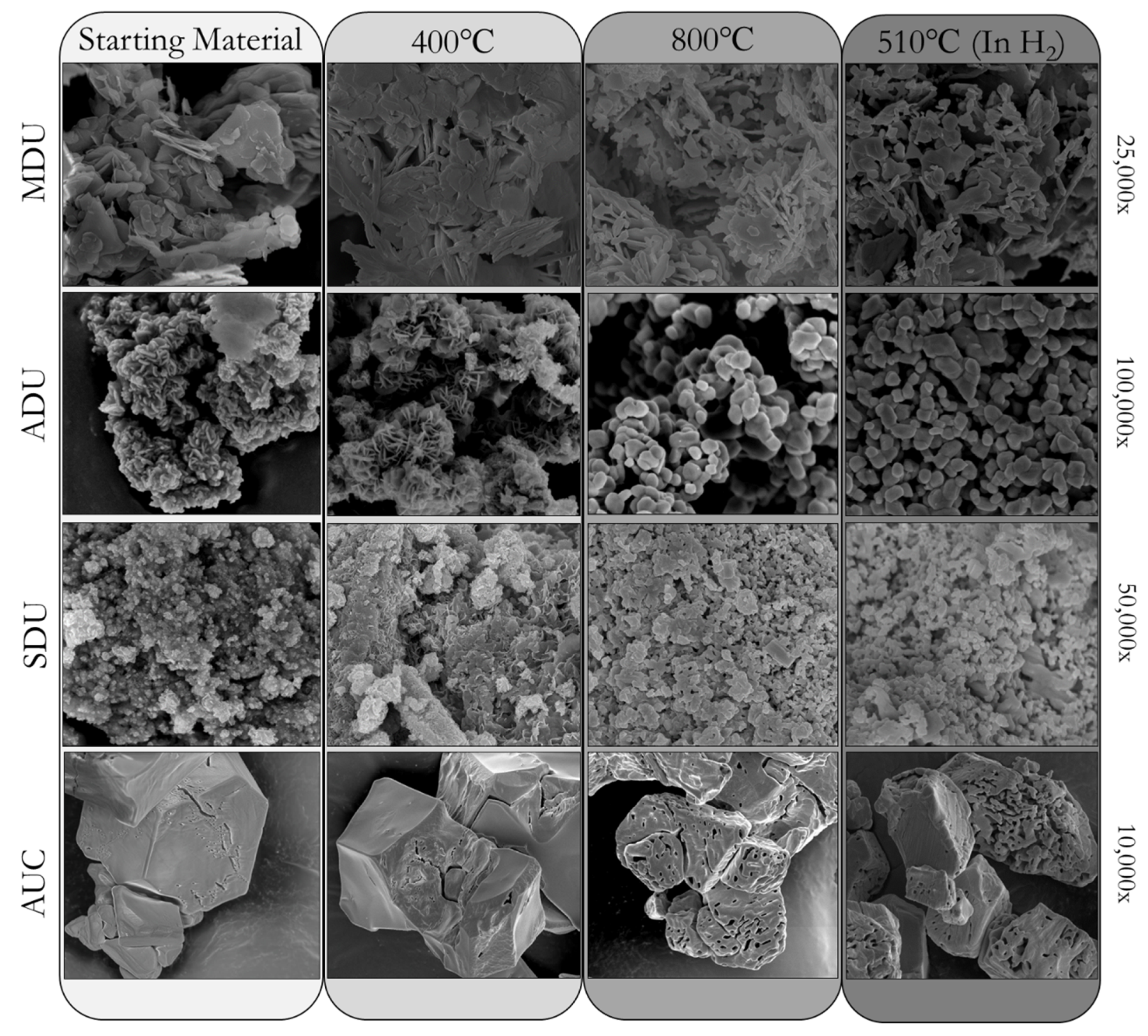
5.1. ABC for ADU, AUC, SDU, MDU
5.2. ABC for the 3 Pathways in ADU, AUC, SDU, MDU
5.3. Model Uncertainty Accommodated by ABC for Inverse Problems in Forensics
6. Discussion and Summary
Author Contributions
Funding
Conflicts of Interest
Appendix A. Morphological Analysis of Materials (MAMA), Software Quantification Attributes
- 1
- Vector AreaThe area of the object calculated using the contour representation, but does not remove any holes. Due to the contour representation passing through the pixels of the perimeter of the object, generally slightly smaller than the pixel area representation.
- 2
- Convex Hull AreaThis is the area contained within the convex hull (convex polygon outline) of the segmented feature.
- 3
- Pixel AreaThis is the area of the object which does not include any holes. This metric is calculated by taking the total number of pixels encapsulated by the object boundary and multiplying by the micrometer/pixel scale.
- 4
- Vector PerimeterThe perimeter of the object using the object contour, calculates the length of the perimeter by summing the lengths of the segments between subsequent points around the boundary as determined by the cvFindCountours function in the OpenCV software.
- 5
- Convex Hull PerimeterThe perimeter of the convex hull of the object.
- 6
- Ellipse PerimeterThe calculated perimeter of the best-fitted ellipse around the boundary of the object using the cvFitEllipse function in the OpenCV software. The major and minor ellipse are extracted from these calculations.
- 7
- Equivalent Circular Diameter (ECD)This is the diameter of a perfect circle that has an area equivalent to the pixel area of the segmented feature. ECD = [4 ∗ (Pixel Area)/π)]1/2
- 8
- Major EllipseMajor ellipse axis calculated from the fitted ellipse from the ellipse perimeter calculations
- 9
- Minor EllipseMinor ellipse axis calculated from the fitted ellipse perimeter calculations
- 10
- Ellipse Aspect RatioThe ratio between the major ellipse and minor ellipse (Major ellipse/minor ellipse)
- 11
- Diameter Aspect RatioFollowing the assignment of a particle boundary to the object, the distance between all pairs of points on the boundary is calculated. The points with the greatest distance between them are assigned the maximum distance chord. Then the pair of points with the greatest distance between them that are within +/− 5 degrees of the orthogonal axis of the maximum distance chord are assigned as the longest orthogonal chord. The ratio of the maximum distance chord and the longest orthogonal chord is the diameter aspect ratio.
- 12
- CircularityA measure of how closely the object perimeter approaches a perfect circle (Circularity=1.0). Calculated from (4 ∗ π ∗ Pixel Area)/(Pixel Perimeter2).
- 13
- Perimeter ConvexityThe ratio of the convex hull perimeter and the object pixel perimeter.
- 14
- Area ConvexityThat ratio of the object area to the convex hull area.
- 15
- Hu Moment 1The image moment is a weighted average of the intensities of the image’s pixels by a set of functions that are invariant to scale, rotation, and translation. The 6 Hu moments were calculated using the cvMoments function in the OpenCV software. The Hu moments are particularly useful for shape matching and pattern recognition of objects from images.
- 16
- Hu Moment 2
- 17
- Hu Moment 3
- 18
- Hu Moment 4
- 19
- Hu Moment 5
- 20
- Hu Moment 6
- 21
- Grayscale meanThe mean of the grayscale intensity values extracted from the all pixels belonging to an object.
- 22
- Gradient MeanThe mean of the gradient magnitudes for each pixel location, which utilized the Sobel operator determined 2D approximate gradient at each pixel location.
Appendix B. ML Options Considered for Classification (as ADU, AUC, SDU, or MDU)
- 1
- Decision TreesCART (classification and regression trees) is among the most versatile and effect ML options, for a categorical response (classification) or continuous response (regression). The R implementation in rpart is versatile and allows recursive partitioning of the predictor space. In addition, Bayesian additive regression trees (BART) as implemented in gbart (generalized BART for continuous and binary outcomes) was applied, but had lower CCR than rpart in R.
- 2
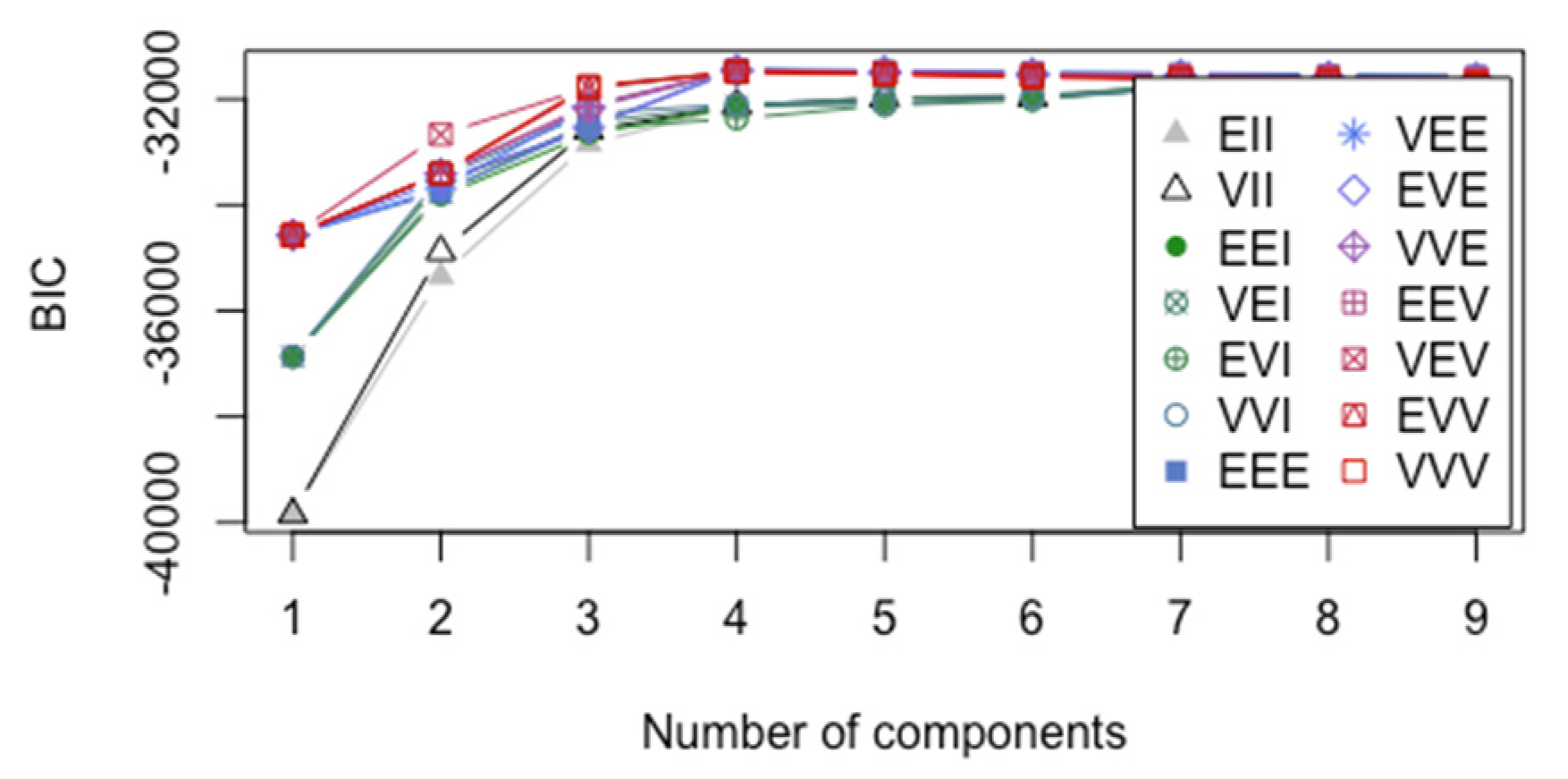
- MDAMixture discriminant analysis as implemented in mclust in R allows several choices for modeling the within-group covariance matrices, as shown in Figure 5.
- 3
- LDA
- 4
- FDAFlexible discriminant analysis uses a mixture of linear regression models, and applies optimal scoring to transform the response variable so that the data are in a better form for linear separation, and multiple adaptive regression splines (MARS) to generate the discriminant surface
- 5
- k-nnNearest-neighbor classification records the group of each of the nearest k neighbors and uses majority rule voting. The choice of k is made by performance on the training data, usually using CV, and the choice of a distance measure to define distances among observations is usually made by trial and error.
- 6
- LVQLearning vector quantization is a neural-network based version of MDA.
- 7
- SVMSupport vector machines can be designed for classification or regression, and seek good class separation (margin) by using hyper-plane separation boundaries.
- 8
- ABCApproximate Bayesian Computation is described for classification in Section 5.
- 9
- MARSMultiple adaptive regression fits a piecewise linear model to capture any nonlinear relationships in the data by choosing cutpoints (knots, as used in spine fits) similar to step functions. MARS is somewhat similar to CART due to the piecewise fitting, and can be performed with categorical responses.
References
- Girard, M.; Hagen, A.; Schwerdt, I.; Gaumer, M.; McDonald, L.; Hodas, N.; Jurrus, E. Uranium Oxide Synthetic Pathway Discernment through Unsupervised Morphological Analysis. J. Nucl. Mater. 2021, 552, 152983. [Google Scholar] [CrossRef]
- Schwerdt, I.; Hawkins, C.; Taylor, B.; Brenkmann, A.; Martinson, S.; McDonald, L. Uranium Oxide Synthetic Pathway Discernment Through Thermal Decomposition and Morphological Analysis. Radiochim. Acta 2019, 107, 193–205. [Google Scholar] [CrossRef]
- Hanson, A.; Schwerdt, I.; Nizinski, C.; Nicholls, R.; Mecham, N.; Abbott, E.; Heffernan, S.; Olsen, A.; Klosterman, M.; Martinson, S.; et al. Impact of Controlled Storage Conditions on the Hydrolysis and Surface Morphology of Amorphous-UO3. ACS Omega 2021, 6, 8605–8615. [Google Scholar] [CrossRef]
- Schwerdt, I.; Olsen, A.; Lusk, R.; Heffernan, S.; Klosterman, M.; Collins, B.; Martinson, S.; Kirkham, T.; McDonald, L. Nuclear Forensics Investigation of Morphological Signatures in the Thermal Decomposition of Uranyl Peroxide. Talanta 2018, 176, 284–292. [Google Scholar] [CrossRef] [PubMed]
- Kim, K.; Hyun, J.; Lee, K.; Lee, E.; Lee, K.; Song, K.; Moon, J. Effects of the Different Conditions of Uranyl and Hydrogen Peroxide Solutions on the Behavior of the Uranium Peroxide Precipitation. J. Hazard. Mater. 2011, 193, 52–58. [Google Scholar] [CrossRef] [PubMed]
- Olsen, A.; Richards, B.; Schwerdt, I.; Heffernan, S.; Lusk, R.; Smith, B.; Jurrus, E.; Ruggiero, C.; McDonald, L. Quantifying Morphological Features of α-U3O8 with Image Analysis for Nuclear Forensics. Anal. Chem. 2017, 89, 3177–3183. [Google Scholar] [CrossRef]
- Schwerdt, I.; Brenkmann, A.; Martinson, S.; Albrecht, B.; Heffernan, S.; Klosterman, M.; Kirkham, T.; Tasdizen, T.; McDonald, L. Nuclear Proliferomics: A New Field of Study to Identify Signatures of Nuclear Materials as Demonstrated on alpha-UO3. Talanta 2018, 186, 433–444. [Google Scholar] [CrossRef]
- Ly, C.; Olsen, A.; Schwerdt, I.; Porter, R.; Sentz, K.; McDonald, L.; Tasdizen, T. A New Approach for Quantifying Morphological Features of U3O8 for Nuclear Forensics Using a Deep Learning Model. J. Nucl. Mater. 2019, 517, 128–137. [Google Scholar] [CrossRef]
- Schwartz, D.; Tandon, L. Uncertainty in the USE of MAMA Software to Measured Particle Morphological Parameters from SEM Images; LAUR-17-24503; Los Alamos National Lab. (LANL): Los Alamos, NM, USA, 2017.
- Gaschen, B.K.; Bloch, J.J.; Porter, R.; Ruggiero, C.E.; Oyen, D.A.; Schaffer, K.M. MAMA User Guide V2.0.1; LA-UR-16-25116; Los Alamos National Lab. (LANL): Los Alamos, NM, USA, 2016.
- Wang, Z. A New Approach for Segmentation and Quantification of Cells or Nanoparticles. IEEE Trans. Ind. Inform. 2016, 12, 962–971. [Google Scholar] [CrossRef]
- R Core Team. R: A Language and Environment for Statistical Computing; R Foundation for Statistical Computing: Vienna, Austria, 2017; Available online: https://www.R-project.org/ (accessed on 11 May 2021).
- Venables, W.; Ripley, B. Modern Applied Statistics with S-Plus; Springer: New York, NY, USA, 1999. [Google Scholar]
- Hastie, T.; Tibshirani, R.; Friedman, J. Elements of Statistical Learning; Springer: New York, NY, USA, 2001. [Google Scholar]
- Miller, R. Beyond ANOVA: The Basics of Applied Statistics; Chapman and Hall: London, UK; CRC Press: Boca Raton, FL, USA, 1997. [Google Scholar]
- Johnson, R.; Wichern, D. Applied Multivariate Statistical Analysis, 2nd ed.; Prentice Hall: Hoboken, NJ, USA, 1992. [Google Scholar]
- Burr, T.; Foy, B.; Fry, H.; McVey, B. Characterizing Clutter in the Context of Detecting Weak Gaseous Plumes in Hyperspectral Imagery. Sensors 2006, 6, 1587–1615. Available online: http://www.mdpi.org/sensors/list06.htm#issue11 (accessed on 11 May 2021). [CrossRef]
- Burr, T.; Croft, S.; Favalli, A.; Krieger, T.; Weaver, B. Bottom-up and Top-Down Uncertainty Quantification for Measurements. Chemom. Intell. Lab. Syst. 2021, 209, 104224. [Google Scholar] [CrossRef]
- Burr, T.; Favalli, A.; Lombardi, M.; Stinnett, J. Application of the Approximate Bayesian Computation Algorithm to Gamma-Ray Spectroscopy. Algorithms 2020, 13, 265. [Google Scholar] [CrossRef]
- Blum, M.; Nunes, M.; Prangle DSisson, S. A Review of Dimension Reduction Methods in Approximate Bayesian Computation. Stat. Sci. 2013, 28, 189–208. [Google Scholar] [CrossRef]
- Nunes MPrangle, D. abctools: An R package for Tuning Approximate Bayesian Computation Analyses. R J. 2016, 7, 189–205. [Google Scholar] [CrossRef] [Green Version]
- Burr, T.; Skurikhin, A. Selecting Summary Statistics in Approximate Bayesian Computation for Calibrating Stochastic Models. BioMed Res. Int. 2013, 2013, 210646. [Google Scholar] [CrossRef] [Green Version]
- Burr, T.; Krieger, T.; Norman, C. Approximate Bayesian Computation Applied to Metrology for Nuclear Safeguards. J. Phys. Conf. Ser. 2018, 57, 50–59. [Google Scholar]
- Carlin, B.; John, B.; Stern, H.; Rubin, D. Bayesian Data Analysis; Chapman and Hall: London, UK; CRC Press: Boca Raton, FL, USA, 1995. [Google Scholar]
- Efron, B. Estimation and Accuracy after Model Selection. J. Am. Stat. Assoc. 2014, 109, 991–1007. [Google Scholar] [CrossRef] [PubMed] [Green Version]
- Lawson, J. Design and Analysis of Experiments in R; Chapman and Hall: London, UK; CRC Press: Boca Raton, FL, USA, 2014. [Google Scholar]
- Lewis, J.; Hang, A.; Anderson-Cook, C. Comparing Multiple Statistical Methods for Inverse Prediction in Nuclear Forensics Applications. Chemom. Intell. Lab. Syst. 2018, 17, 116–129. [Google Scholar] [CrossRef]
- Lu, L.; Anderson-Cook, C. Strategies for Sequential Design of Experiments and Augmentation. Qual. Reliab. Eng. 2020, 2020, 1740–1757. [Google Scholar] [CrossRef]
- Myers, R.; Montgomery, D. Response Surface Methodology; Wiley: Hoboken, NJ, USA, 1995. [Google Scholar]
- Silvestrini RMontgomery, D.; Jones, B. Comparing Computer Experiments for the Gaussian Process Model Using Integrated Prediction Variance. Qual. Eng. 2013, 25, 164–174. [Google Scholar] [CrossRef]
- Thomas, E.; Lewis, J.; Anderson-Cook, A.; Burr, T.; Hamada, M.S. Selecting an Informative/Discriminating Multivariate Response for Inverse Prediction. J. Qual. Technol. 2017, 49, 228–243. [Google Scholar] [CrossRef]


| Tree | MDA | LDA | FDA | knn | LVQ | SVM | ABC | MARS | |
|---|---|---|---|---|---|---|---|---|---|
| 3 pathways | 0.83 | 0.76 | 0.74 | 0.74 | 0.81 | 0.75 | 0.76 | 0.87 | 0.87 |
| 1 pathway | 0.93 | 0.82 | 0.81 | 0.81 | 0.85 | 0.87 | 0.83 | 0.89 | 0.89 |
Publisher’s Note: MDPI stays neutral with regard to jurisdictional claims in published maps and institutional affiliations. |
© 2021 by the authors. Licensee MDPI, Basel, Switzerland. This article is an open access article distributed under the terms and conditions of the Creative Commons Attribution (CC BY) license (https://creativecommons.org/licenses/by/4.0/).
Share and Cite
Burr, T.; Schwerdt, I.; Sentz, K.; McDonald, L.; Wilkerson, M. Overview of Algorithms for Using Particle Morphology in Pre-Detonation Nuclear Forensics. Algorithms 2021, 14, 340. https://doi.org/10.3390/a14120340
Burr T, Schwerdt I, Sentz K, McDonald L, Wilkerson M. Overview of Algorithms for Using Particle Morphology in Pre-Detonation Nuclear Forensics. Algorithms. 2021; 14(12):340. https://doi.org/10.3390/a14120340
Chicago/Turabian StyleBurr, Tom, Ian Schwerdt, Kari Sentz, Luther McDonald, and Marianne Wilkerson. 2021. "Overview of Algorithms for Using Particle Morphology in Pre-Detonation Nuclear Forensics" Algorithms 14, no. 12: 340. https://doi.org/10.3390/a14120340
APA StyleBurr, T., Schwerdt, I., Sentz, K., McDonald, L., & Wilkerson, M. (2021). Overview of Algorithms for Using Particle Morphology in Pre-Detonation Nuclear Forensics. Algorithms, 14(12), 340. https://doi.org/10.3390/a14120340