A New Chaotic-Based Approach for Multi-Objective Optimization

Abstract

Multi-objective optimization problems (MOPs) have been widely studied during the last decades. In this paper, we present a new approach based on Chaotic search to solve MOPs. Various Tchebychev scalarization strategies have been investigated. Moreover, a comparison with state of the art algorithms on different well known bound constrained benchmarks shows the efficiency and the effectiveness of the proposed Chaotic search approach.

1. Introduction

Many problems in science and industry are concerned with multi-objective optimization problems (MOPs). Multi-objective optimization seeks to optimize several components of an objective function vector. Contrary to single-objective optimization, the solution of a MOP is not a single solution, but a set of solutions known as Pareto optimal set, which is called Pareto front when it is plotted in the objective space. Any solution of this set is optimal in the sense that no improvement can be made on a component of the objective vector without worsening at least another of its components. The main goal in solving a difficult MOP is to approximate the set of solutions within the Pareto optimal set and, consequently, the Pareto front.

Definition 1

(MOP). A multi-objective optimization problem (MOP) may be defined as:

$$\begin{array}{cc}\left(MOP\right)=\hfill & \left\{\begin{array}{c}minF\left(x\right)=(f_1\left(x\right),f_2\left(x\right),\cdots ,f_k\left(x\right))\hfill \\ s.c.x\in X\hfill \end{array}\right.\hfill \end{array}$$

(1)

where k $(k\ge 2)$ is the number of objectives, $x=(x_1\dots ,x_n)$ is the vector representing the decision variables, and X represents the set of feasible solutions associated with equality and inequality constraints, and explicit bounds. $F\left(x\right)=(f_1\left(x\right),f_2\left(x\right)\dots ,f_k\left(x\right))$ is the vector of objectives to be optimized.

The set of all values satisfying the constraints defines the feasible region X and any point $\overrightarrow{x}\in X$ is a feasible solution. As mentioned before, we seek for the Pareto optima.

Definition 2

(Pareto). A point ${\overrightarrow{x}}^{*}\in X$ is Pareto Optimal if for every $\overrightarrow{x}\in X$ and $I=\left\{1,2,\dots ,k\right\}$${\forall }_{i\in I}\left(f_i\left(\overrightarrow{x}\right)\ge f_i({\overrightarrow{x}}^{*}\right)$ and there is at least one $i\in I$ such that $f_i\left(\overrightarrow{x}\right)>f_i\left({\overrightarrow{x}}^{*}\right)$.

This definition states that ${\overrightarrow{x}}^{*}$ is Pareto optimal if no feasible vector $\overrightarrow{x}$ exists which would improve some criterion without causing a simultaneous worsening in at least one other criterion.

Definition 3

(Dominance). A vector $\overrightarrow{u}=\left(u_1,\dots ,u_n\right)$ is said to dominate $\overrightarrow{v}=\left(v_1,\dots ,v_n\right)$ (denoted by $\overrightarrow{u}\preccurlyeq \overrightarrow{v}$) if and only if $\overrightarrow{u}$ is partially less than $\overrightarrow{v}$, i.e., $\forall i\in \left\{1,\dots ,n\right\},u_i\le v_i\wedge \exists i\in \left\{1,\dots ,k\right\}:u_i<v_i.$

Definition 4

(Pareto set). For a given MOP $\overrightarrow{f}\left(\overrightarrow{x}\right)$, the Pareto optimal set is defined as ${\mathcal{P}}^{*}=\{\overrightarrow{x}\in X|\neg \exists \overrightarrow{x^{\prime }}\in X,\overrightarrow{f}(\overrightarrow{x^{\prime }})\preccurlyeq \overrightarrow{f}\left(\overrightarrow{x}\right)\}$.

Definition 5

(Pareto front). For a given MOP $\overrightarrow{f}\left(\overrightarrow{x}\right)$ and its Pareto optimal set ${\mathcal{P}}^{*}$, the Pareto front is defined as ${\mathcal{PF}}^{*}=\{\overrightarrow{f}\left(\overrightarrow{x}\right),\overrightarrow{x}\in {\mathcal{P}}^{*}\}$.

Definition 6

(Reference point). A reference point $z^{*}=\left[{\overline{z}}_1,{\overline{z}}_2,\dots ,{\overline{z}}_n\right]$ is a vector which defines the aspiration level (or goal) ${\overline{z}}_i$ to reach for each objective $f_i$.

Definition 7

(Nadir point). A point $y^{*}=(y_1^{*},y_2^{*},\dots ,y_n^{*})$ is the nadir point if it maximizes each objective function $f_i$ of F over the Pareto set, i.e., $y_i^{*}=max\left(f_i\left(x\right)\right),x\in {\mathcal{P}}^{*},i\in [1,n]$.

The approaches developed for treating optimization problems can be mainly divided into deterministic and stochastic. Deterministic methods (e.g., linear programming, nonlinear programming, and mixed-integer nonlinear programming, etc.) provide a theoretical guarantee of locating the global optimum or at least a good approximation of it whereas the stochastic methods offer a guarantee in probability [1,2,3].

Most of the well-known metaheuristics (e.g., evolutionary algorithms, particle swarm, ant colonies) have been adapted to solve multi-objective problems [4,5] with a growing number of applications [6,7,8].

Multi-objective metaheuristics can be classified in three main categories:

• Scalarization-based approaches: this class of multi-objective metaheuristics contains the approaches which transform a MOP problem into a single-objective one or a set of such problems. Among these methods one can find the aggregation methods, weighted metrics, cheybycheff method, goal programming methods, achievement functions, goal attainment methods and the $ϵ$-constraint methods [9,10].
• Dominance-based approaches: the dominance-based approaches (Also named Pareto approaches.) use the concept of dominance and Pareto optimality to guide the search process. Since the beginning of the nineties, interest concerning MOPs area with Pareto approaches always grows. Most of Pareto approaches use EMO (Evolutionary Multi-criterion Optimization) algorithms. Population-based metaheuristics seem particularly suitable to solve MOPs, because they deal simultaneously with a set of solutions which allows to find several members of the Pareto optimal set in a single run of the algorithm. Moreover, they are less sensitive to the shape of the Pareto front (continuity, convexity). The main differences between the various proposed approaches arise in the followins search components: fitness assignment, diversity management, and elitism [11].
• Decomposition-based approaches: most of decomposition based algorithms in solving MOPs operate in the objective space. One of the well-known frameworks for MOEAs using decomposition is MOEOA/D [12]. It uses scalarization to decompose the MOP into multiple scalar optimization subproblems and solve them simultaneously by evolving a population of candidate solutions. Subproblems are solved using information from the neighbouring subproblems [13].

We are interested in tackling MOPs using Chaotic optimization approaches. In our previous work, we proposed a efficient metaheuristic for single objective optimization called Tornado which is based on Chaotic search. It is a metaheuristic developed to solve large-scale continuous optimization problems. In this paper we extend our Chaotic approach Tornado to solve MOPs by using various Tchebychev scalarization approaches.

The paper is organized as follow. Section 1 recalls the main principles of the Chaotic search Tornado algorithm. Then the extended Chaotic search for multi-objective optimization is detailed in Section 3. In Section 4 the experimental settings and computational results against competing methods are detailed and analyzed. Finally, the Section 5 concludes and presents some future works.

2. The Tornado Chaotic Search Algorithm

2.1. Chaotic Optimization Algorithm: Recall

The chaotic optimization algorithm (COA) is recently proposed metaheuristic method [14] which is based on chaotic sequences instead of random number generators and mapped as the design variables for global optimization. It includes generally two main stages:

• Global search: This search corresponds to exploration phase. A sequence of chaotic solutions is generated using a chaotic map. Then, this sequence is mapped into the range of the search space to get the decision variables on which the objective function is evaluated and the solution with the best objective function is chosen as the current solution.
• Local search: After the exploration of the search space, the current solution is assumed to be close to the global optimum after a given number of iterations, and it is viewed as the centre on which a little chaotic perturbation, and the global optimum is obtained through local search. The above two steps are iterated until some specified stopping criterion is satisfied.

In recent years COA has attracted widespread attention and have been widely investigated and many choatic approaches have been proposed in the litterature [15,16,17,18,19,20,21].

2.2. Tornado Principle

The Tornado algorithm has been as an improvement to the basic COA approach to correct some of major drawbacks such as the inability of the method to deal with high-dimensional problems [22,23]. Indeed, the Tornado algorithm introduces new strategies such as symmetrization and levelling of the distribution of chaotic variables in order to break the rigidity inherent in chaotic dynamics.

The proposed Tornado algorithm is composed of three main procedures:

• The chaotic global search (CGS): this procedure explores the entire research space and select the best point among a distribution of symmetrized distribution of chaotic points.
• The chaotic local search (CLS): The CLS carries out a local search on neighbourhood of the solution initially found CGS, it exploits the of the solution. Moreover, by focusing on successive promising solutions, CLS allows also the exploration of promising neighboring regions.
• The chaotic fine search (CFS): It is programmed after the CGS and CLS procedures in order to refine their solutions by adopting a coordinate adaptive zoom strategy to intensify the search around the current optimum.

As a COA approach, The Tornado algorithm relies on a chaotic sequence in order to generate chaotic variables that will be used in the search process. For instance, Henon map was adopted as a generator of a chaotic sequence in Tornado.

To this end. We consider a sequence ${\left(Z_k\right)}_{1\le k\le N_h}$ of normalized Henon vectors $Z_k=(z_{k,1},z_{k,2},\dots ,z_{k,n})\in {\mathrm{I}\mathrm{R}}^n$ built by the following linear transformation of the standard Henon map [24]:

$$z_{k,i}=\frac{y_{k,i}-{\alpha }_i}{{\beta }_i-{\alpha }_i},\forall (k,i)\in \left[[1,N_h]\right]\times \left[[1,n]\right],$$

(2)

where ${\alpha }_i={min}_k\left(y_{k,i}\right)$ and ${\beta }_i={max}_k\left(y_{k,i}\right).$

Thus, we obtain $\forall (k,i)\in \left[[1,N_h]\right]\times \left[[1,n]\right],0⩽z_{k,i}⩽1$. In this paper, the parameters of the Henon map sequence $\left(Z_k\right)$ are set as follows:

$a=1.5,b=0.2,\forall k\in \left[[1,n]\right],(x_{{}_{k,0}},y_{{}_{k,0}})=(r_k,0),r_k\sim U(0,1).$

The structure of the proposed Tornado approach is given in Algorithm 1.

Algorithm 1 The Tornado algorithm structure.

Initialization of the Henon chaotic sequence; Set $k=1$; Repeat    Chaotic Global Search (CGS);    Set $s=1$;    Repeat;      Chaotic Local Search (CLS);      Chaotic Finest Search (CFS);      $s=s+1$;    Until $s=M_l$; /* ${\mathrm{M}}_l$ is the number of CLS/CFS by cycle */    $k=k+1$; Until$k=M$; /* $\mathrm{M}$ is maximum number of cycles of Tornado */

2.2.1. Chaotic Global Search (CGS)

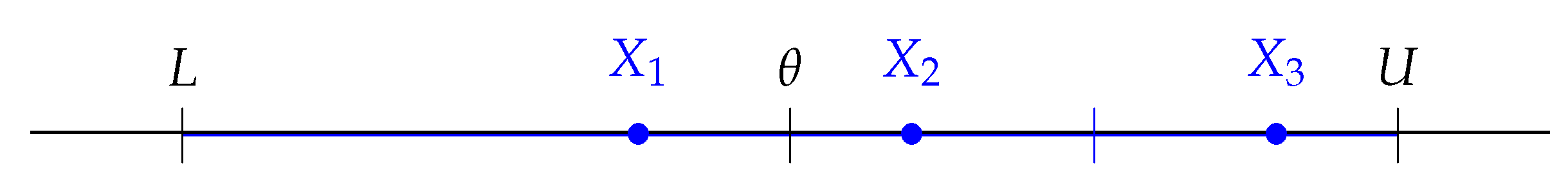
CGS starts by mapping the chaotic sequence generated by the adopted standard Henon map variable Z into ranges of design variable X by considering the following transformations (Figure 1):

$$X_1=L+Z(U-L).X_2=\theta +Z(U-\theta ),X_3=U-Z(U-\theta ),\theta =\frac{1}{2}(L+U).$$

(3)

Those proposed transformations aim to overcome the inherent rigidity of the chaos dynamics.

• Levelling approach: In order to provide more diversification in the chaotic distribution, CGS proceeds by levelling with $N_c$ chaotic levels. In each chaotic level $l\in$$\left[[1,N_c]\right]$, and for each iteration k three chaotic variables are generated through the following formulas:

  $$X_1=L+(U-L)\times Z_{k+(l-1)N_c}$$

  (4)

  $$X_2=\theta +(U-\theta )\times Z_{k+(l-1)N_c}$$

  (5)

  $$X_3=U-(U-\theta )\times Z_{k+(l-1)N_c}$$

  (6)
  Note that for sake of simplicity, henceforth $X_{i,k}$ will be simply noted $X_i$.
• Symmetrization approach: In high-dimensional space, the exploration of all the dimensions is not practical because of combinatorial explosion. To get around this difficulty, we have introduced a new strategy based on a stochastic decomposition of the search space ${\mathbb{R}}^{\mathit{n}}$ into two vectorial subspaces: a vectorial line $\mathcal{D}$ and its corresponding hyperplane $\mathcal{H}$:

  $${\displaystyle {\mathrm{I}\mathrm{R}}^n=\mathcal{D}\oplus \mathcal{H},\mathcal{D}=\mathrm{I}\mathrm{R}\times e_p,\mathcal{H}=\mathrm{vect}{\left(e_i\right)}_{i\ne p}}.$$

  (7)
  By consequence,

  $$\forall X=(x_1,x_2,\dots ,x_n)\in {\mathrm{I}\mathrm{R}}^n:X=X_d+X_h,$$

  (8)

  where

  $$X_d=(0,\cdots ,0,x_p,0,\cdots ,0)\in \mathcal{D},X_h=(x_1,\cdots ,x_{p-1},0,x_{p+1},\cdots ,x_n)\in \mathcal{H}.$$

  (9)

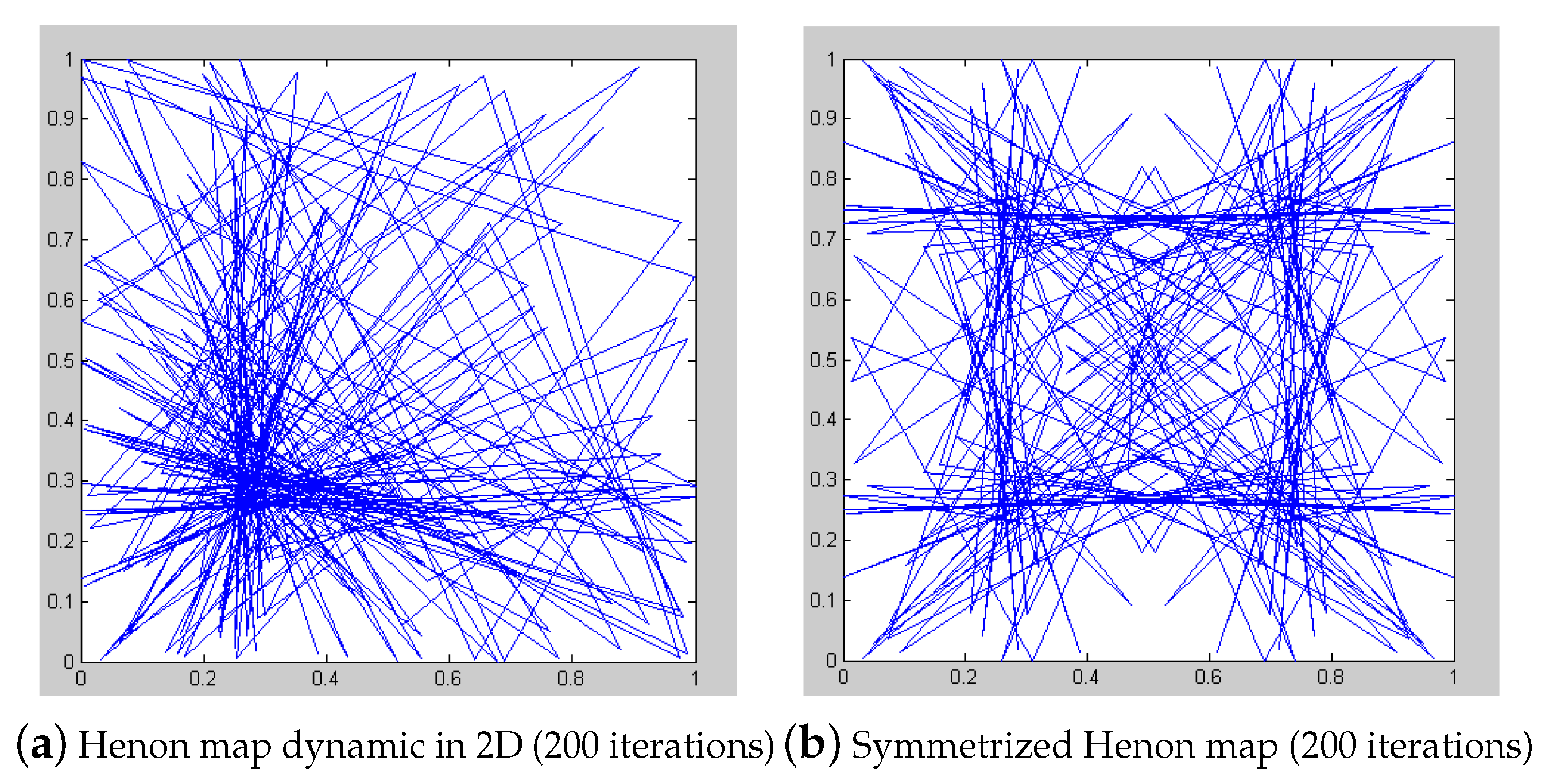
The symmetrization approach based on this stochastic decomposition of the design space offers two significant advantages:

∘

Significant reduction of complexity in the high dimensional problem in a way as if we were dealing with a 2D space with four directions.

∘

The symmetric chaos is more regular and more ergodic than the basic one (Figure 2).

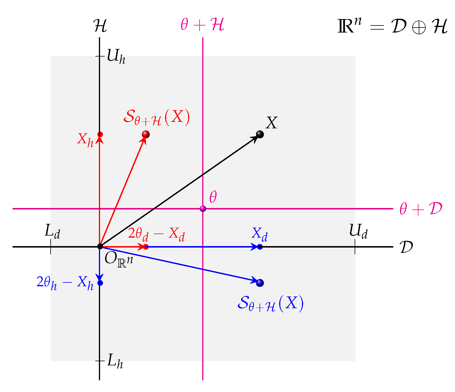
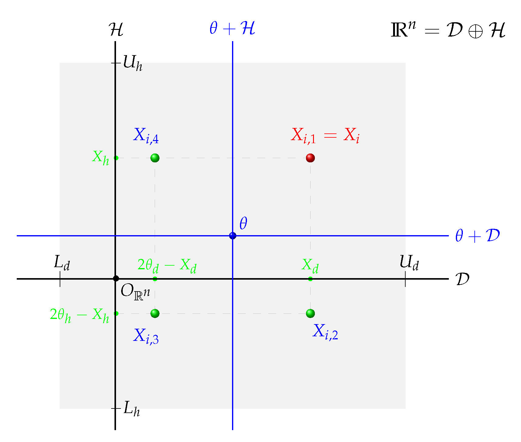
Thanks to the stochastic decomposition (Equation (7)), CGS generates four symmetric chaotic points using axial symmetries ${\mathcal{S}}_{\theta +\mathcal{D}},{\mathcal{S}}_{\theta +\mathcal{H}}$ (Figure 3):

$$\begin{array}{cccc}{X}_{i,1}\hfill & =X_i,\hfill & X_{i,2}\hfill & ={\mathcal{S}}_{\theta +\mathcal{D}}\left(X_{i,1}\right),\hfill \\ X_{i,3}\hfill & ={\mathcal{S}}_{\theta +\mathcal{H}}\left(X_{i,2}\right),\hfill & X_{i,4}\hfill & ={\mathcal{S}}_{\theta +\mathcal{D}}\left(X_{i,3}\right)={\mathcal{S}}_{\theta +\mathcal{H}}\left(X_{i,1}\right),\hfill \end{array}$$

(10)

where the axial symmetries ${\mathcal{S}}_{\theta +\mathcal{D}},{\mathcal{S}}_{\theta +\mathcal{H}}$ are defined as follows:

$$\begin{array}{c}\hfill {\mathcal{S}}_{\theta +\mathcal{D}}\left(X\right)=X_d+(2{\theta }_h-X_h)\end{array}$$

(11)

$$\begin{array}{c}\hfill {\mathcal{S}}_{\theta +\mathcal{H}}\left(X\right)=(2{\theta }_d-X_d)+X_h\end{array}$$

(12)

In other words, $\forall i\in \{1,2,3\}$:

$$\begin{array}{cccc}{X}_{i,1}\hfill & =X_i=X_{i,d}+X_{i,h},\hfill & X_{i,2}\hfill & =X_{i,d}+2{\theta }_h-X_{i,h},\hfill \\ X_{i,3}\hfill & =2\theta -X_{i,1},\hfill & X_{i,4}\hfill & =2\theta -X_{i,2}.\hfill \end{array}$$

(13)

At last, the best solution among these all generated chaotic points is selected as illustrated by Figure 4.

The code of CGS is detailed in Algorithm 2.

Algorithm 2 Chaotic global search (CGS).

1: Input: $f,U,Z,N_{\mathrm{c}},k$ 2: Output: $X_{\mathrm{c}}$ 3: $Y=+\infty ;$$\theta =\frac{1}{2}(U+L)$ 4: for$l=1$ to $N_{\mathrm{c}}$ 5:    Generate 3 chaotic variables $X_1,X_2,$ and $X_3$ according to (Equations (4)–(6)) 6:    for   $i=1$   to   3 7:     Select randomly an index $p\in \{1,\cdots ,n\}$ and decompose $X_i$ according to (Equation (8)) 8:     Generate the 4 corresponding symmetric points ${\left(X_{i,j}\right)}_{1⩽j⩽4}$ according to (Equations (10)–(13)) 9:        for $j=1$  to  4      10:             if $Y>f\left(X_{i,j}\right)$ 11:                $X_c=X_{i,j};$ $Y=f\left(X_{i,j}\right)$ 12:             end if 13:        end for 14:    end for 15: end for

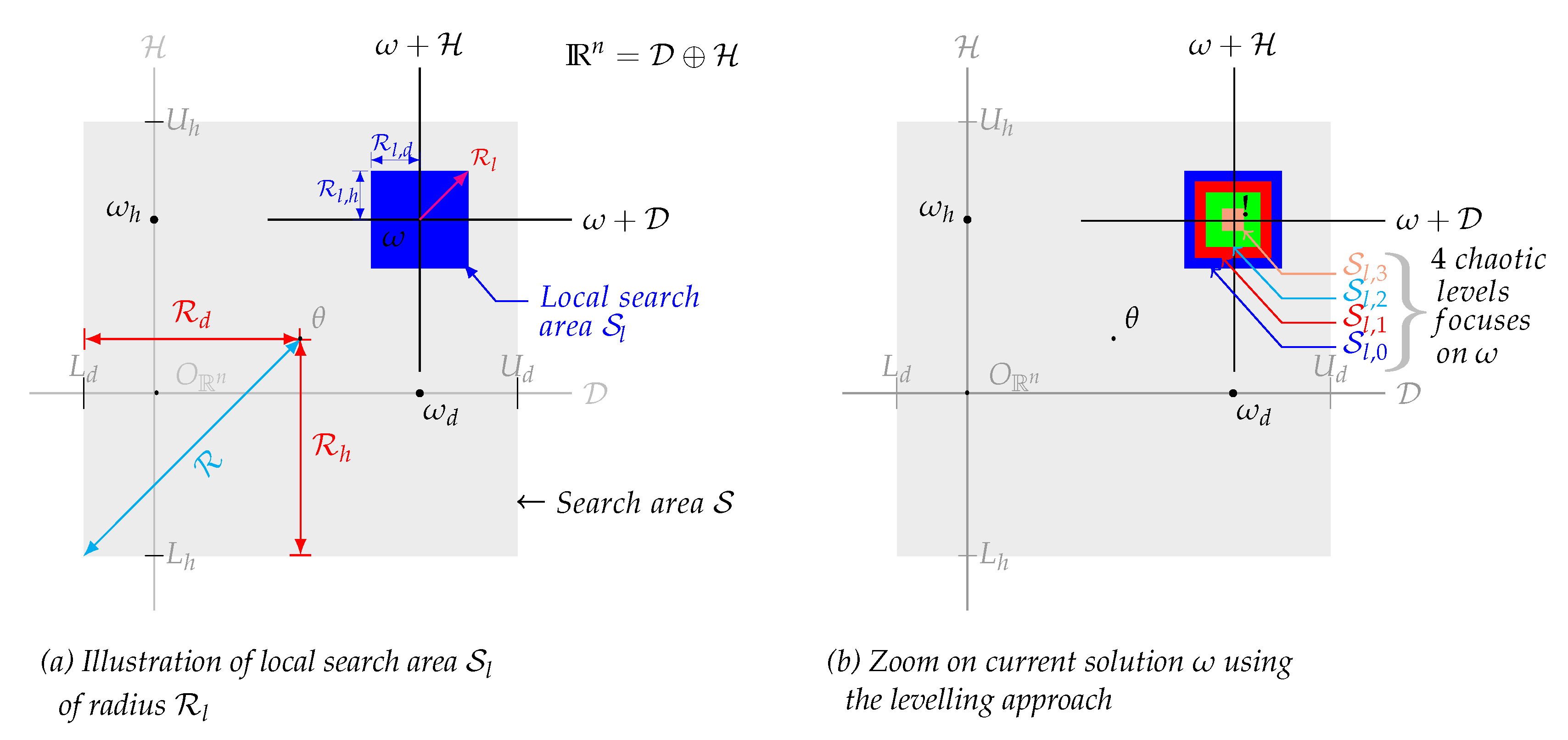
2.2.2. Chaotic Local Search (CLS)

The CLS procedure is designed to refine the search by exploiting the neighborhood of the solution $\mathit{\omega }$ found by the chaotic global search CGS. In fact, the search process is conducted near the current solution $\omega$ within a local search area ${\mathcal{S}}_{\mathbf{l}}$ whose radius is ${\mathcal{R}}_{\mathbf{l}}=r\times \mathcal{R}$ focused on $\omega$ (see Figure 5a), where $r\sim U(0,1)$ is a random parameter that corresponds to the reduction rate, and $\mathcal{R}$ denotes the radius of the search zone $\mathcal{S}={\displaystyle \prod _{i=1}^n}\left[l_i,u_i\right]$ such as:

$$\mathcal{R}=\frac{1}{2}(U-L)=\left(\frac{1}{2}(u_1-l_1),\dots ,\frac{1}{2}(u_n-l_n)\right)$$

(14)

The CLS procedure uses the following strategy to produce chaotic variables:

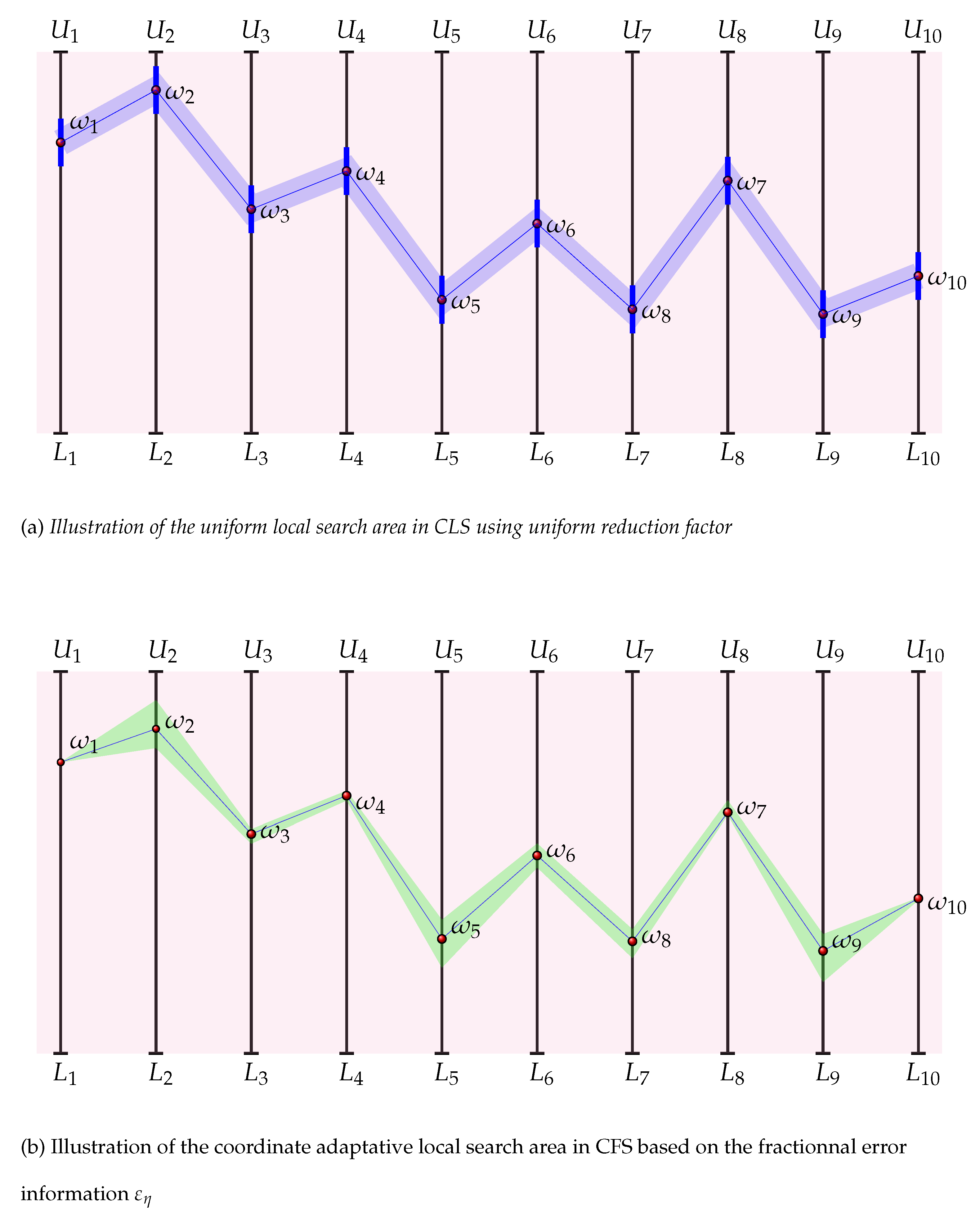
• Like the CGS, the CLS also involves a levelling approach by creating $N_{\mathrm{l}}$ chaotic levels focused on $\omega$. The local search process in each chaotic level $\eta \in$$\left[[0,N_l-1]\right]$, is limited to a local area ${\mathcal{S}}_{l,\eta }$ focused on $\omega$ (see Figure 5b) characterized by its radius ${\mathcal{R}}_{\eta }$ defined by the following:

  $${\mathcal{R}}_{\eta }={\gamma }_{\eta }\times {\mathcal{R}}_l=r\times {\gamma }_{\eta }\times \mathcal{R},$$

  (15)

  where ${\gamma }_{\eta }$ is a decreasing parameter through levels which we have formulated in this work as follows:

  $${\gamma }_{\eta }={\displaystyle \frac{{10}^{-2s\eta }}{1+\eta }},s\sim U(0,1)$$

  (16)
  This levelling approach used by the CLS can be interpreted as a progressive zoom focus on the current solution $\omega$ carried out through $N_{\mathrm{l}}$ chaotic levels, and ${\gamma }_{\eta }$ is the factor indicating the speed of this zoom process $({\gamma }_{\eta }\searrow 0)$ (see Figure 5b).
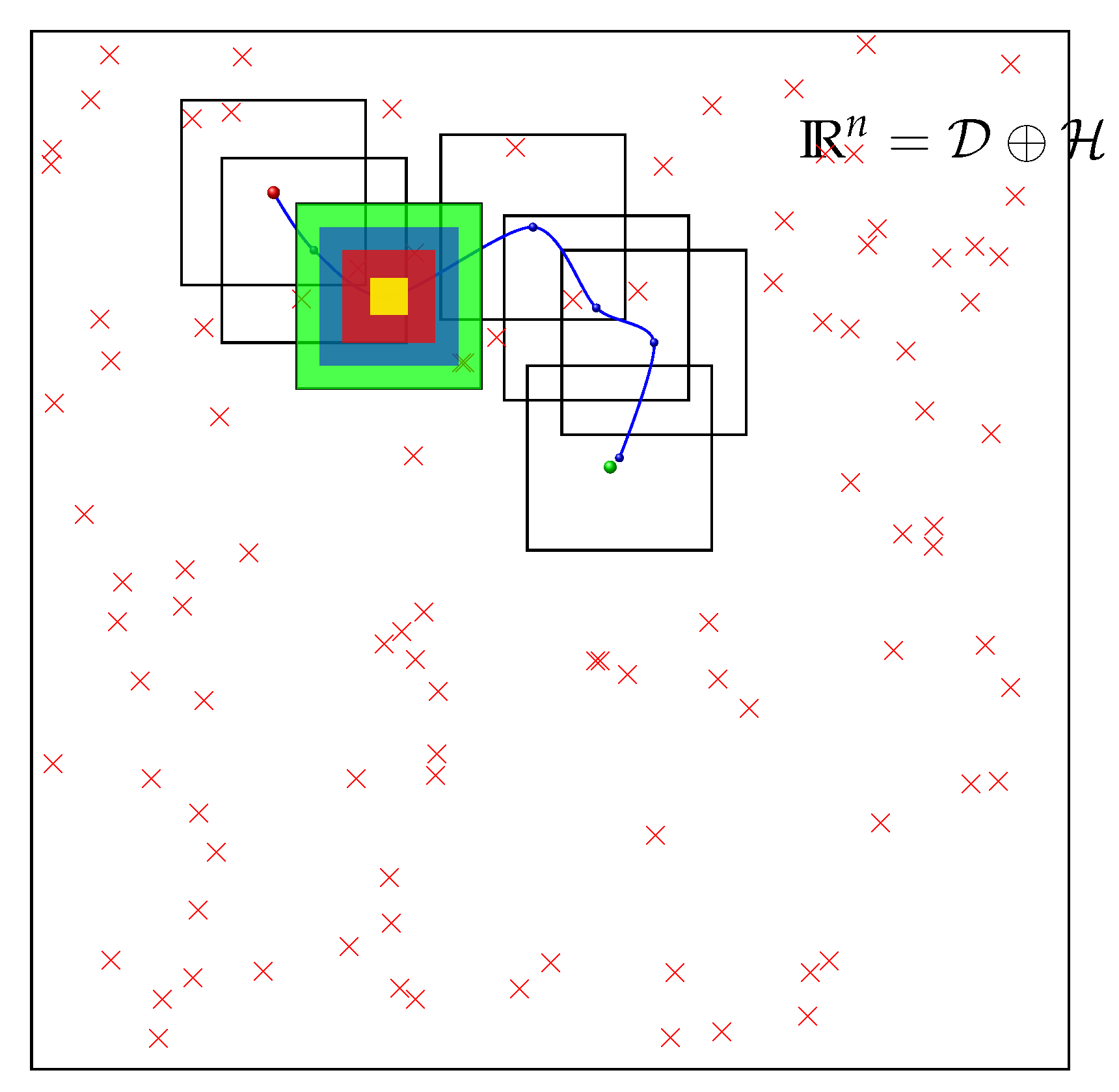
  Furthermore, by looking for potential solutions relatively far from the current solution CLS contributes also to the exploration of the decision space. Indeed, once the CGS provides an initial solution $\omega$, the CLS intensifies the search around this solution, through several chaotic layers. After each CGS run, CLS carry out several cycles of local search (i.e., $M_l$) This way, the CLS participates also to the exploration of neighboring regions by following the zoom dynamic through the CLS cycles as shown in Figure 6.
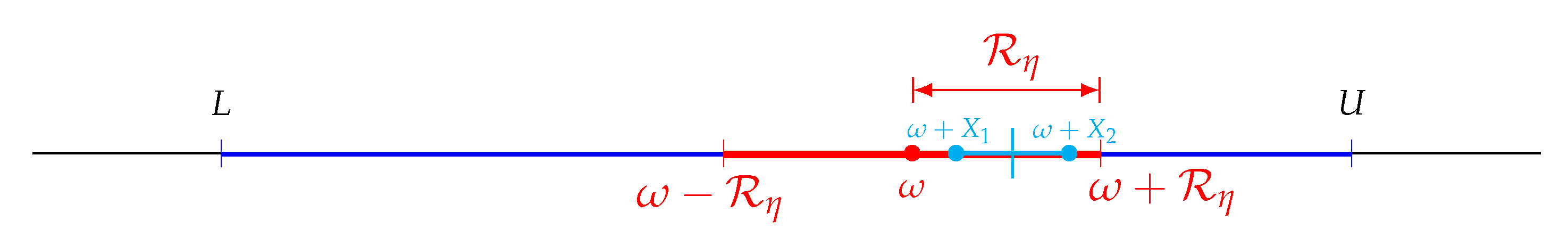
• Moreover, in each chaotic level $\eta$, CLS creates two symmetric chaotic variables $X_1,X_2$ defined as follows (Figure 7):

  $$X_1=Z\times {\mathcal{R}}_{\eta },X_2=(1-Z)\times {\mathcal{R}}_{\eta }={\mathcal{R}}_{\eta }-X_1.$$

  (17)
  By randomly choosing an index $p\in \{1,\dots ,n\}$ a stochastic decomposition of ${\displaystyle {\mathrm{I}\mathrm{R}}^n}$ is built given by:

  $${\displaystyle {\mathrm{I}\mathrm{R}}^n=\mathcal{D}\oplus \mathcal{H},\mathcal{D}=\mathrm{I}\mathrm{R}\times e_p,\mathcal{H}=\mathrm{vect}{\left(e_i\right)}_{i\ne p}}.$$

  (18)
  Based on this, a decomposition of each chaotic variable $X_{i,(i=1,2)}$ is applied:

  $$X_i=X_{i,d}+X_{i,h}.$$

  (19)
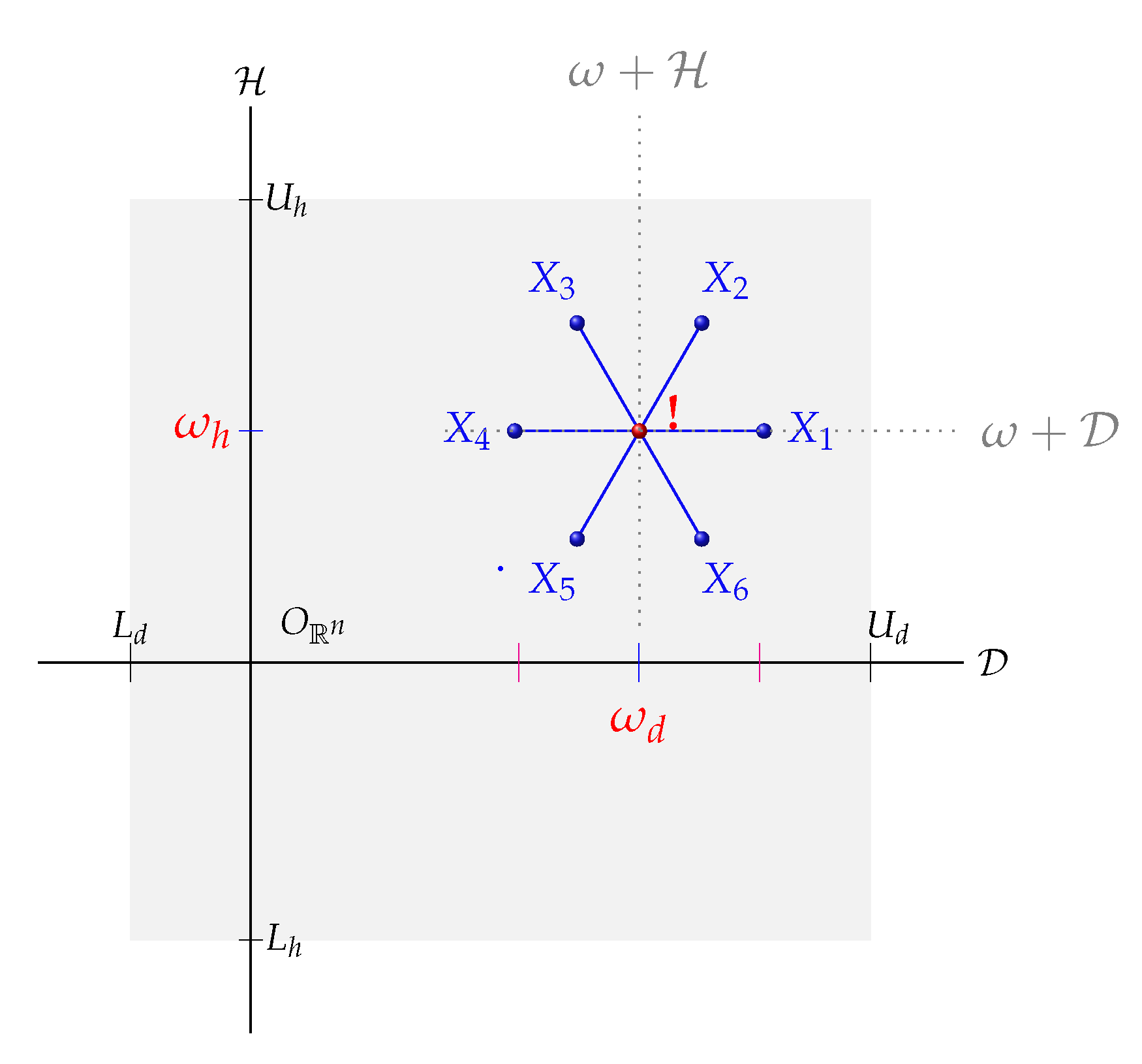
  Finally, from each chaotic variable $X_{i,(i=1,2)}$, $N_p$ symmetric chaotic points ${\left(X_{i,j}\right)}_{{}_{1⩽j⩽N_p}}$ are generated using the polygonal model (Figure 8): polygonal model

  $$\begin{array}{cc}{X}_{i,j}\hfill & =\omega +X_i=\omega +cos(2\pi .j/N_p)X_{i,d}+sin(2\pi .j/N_p)X_{i,h},\hfill \end{array}$$

  (20)

Moreover, if $\omega$ is close enough to the borders of the search area $\mathcal{S}$, the search process risks to leave it and then may give an infeasible solution localized outside $\mathcal{S}$.

Indeed, that particularly happens in case of ${\mathcal{R}}_{\eta ,i}>d_B\left({\omega }_i\right)$ for at least one component ${\omega }_i$ (Figure 9), where $d_{\mathrm{B}}\left({\omega }_i\right)$ is the distance of the component ${\omega }_i$ to borders $l_i,u_i$ defined as follows:

$$d_{\mathrm{B}}\left({\omega }_i\right)=min(u_i-{\omega }_i,{\omega }_i-l_i).$$

(21)

To prevent this overflow, the local search radius ${\mathcal{R}}_{\eta }$ is corrected through the the following formula:

$${\tilde{R}}_{\eta }=min({\mathcal{R}}_{\eta },d_{\mathrm{B}}\left(\omega \right)),$$

(22)

where $d_{\mathrm{B}}\left(\omega \right)=(d_{\mathrm{B}}\left({\omega }_1\right),\dots ,d_{\mathrm{B}}\left({\omega }_n\right))$. This ensures ${\tilde{R}}_{\eta ,i}⩽d_{\mathrm{B}}\left({\omega }_i\right),\forall i\in \left[\left[1,n\right]\right]$. Hence, Equation (17) become

$$X_1=Z\times {\tilde{R}}_{\eta },X_2=(1-Z)\times {\tilde{R}}_{\eta }.$$

(23)

Finally, the chaotic local search (CLS) code is detailed in Algorithm 3.

Algorithm 3 Chaotic Local Search (CLS).

1: Input: $\mathit{f},\mathit{\omega },\mathit{L},\mathit{U},\mathit{Z},{\mathit{N}}_{\mathit{l}},{\mathit{N}}_{\mathit{p}}$ 2: Output: $X_l$: best solution among the local chaotic points 3: $\mathcal{R}=\frac{1}{2}(U-L);{\mathcal{R}}_l=r\times \mathcal{R};$ 4: $X=\omega ;$ 5: $X_l=\omega ;Y=f\left(\omega \right);$ 6: for$\eta =0$  to $N_l-1$ 7:  Set ${\mathcal{R}}_{\eta }={\gamma }_{\eta }\times {\mathcal{R}}_l,$ and then compute ${\tilde{R}}_{\eta }=min\left({\mathcal{R}}_{\eta },d_B\left(\omega \right)\right)$ 8:  Generate 2 symmetric chaotic variables $X_1$,  $X_2$ according to (23) 9:  for  $i=1$  to  2 10:    Select an index $p\in \{1,\dots ,n\}$ randomly and decompose $X_i$ according to (19) 11:    Generate the $N_p$ corresponding symmetric points $X_{i,j}$ according to (20) 12:       for $j=1$  to  $N_p$ 13:           if   $Y>f\left(X_{i,j}\right)$   then 14:                $X_l=X_{i,j};Y=f\left(X_{i,j}\right);$ 15:           end if 16:       end for 17:   end for 18: end for

2.2.3. Chaotic Fine Search (CFS)

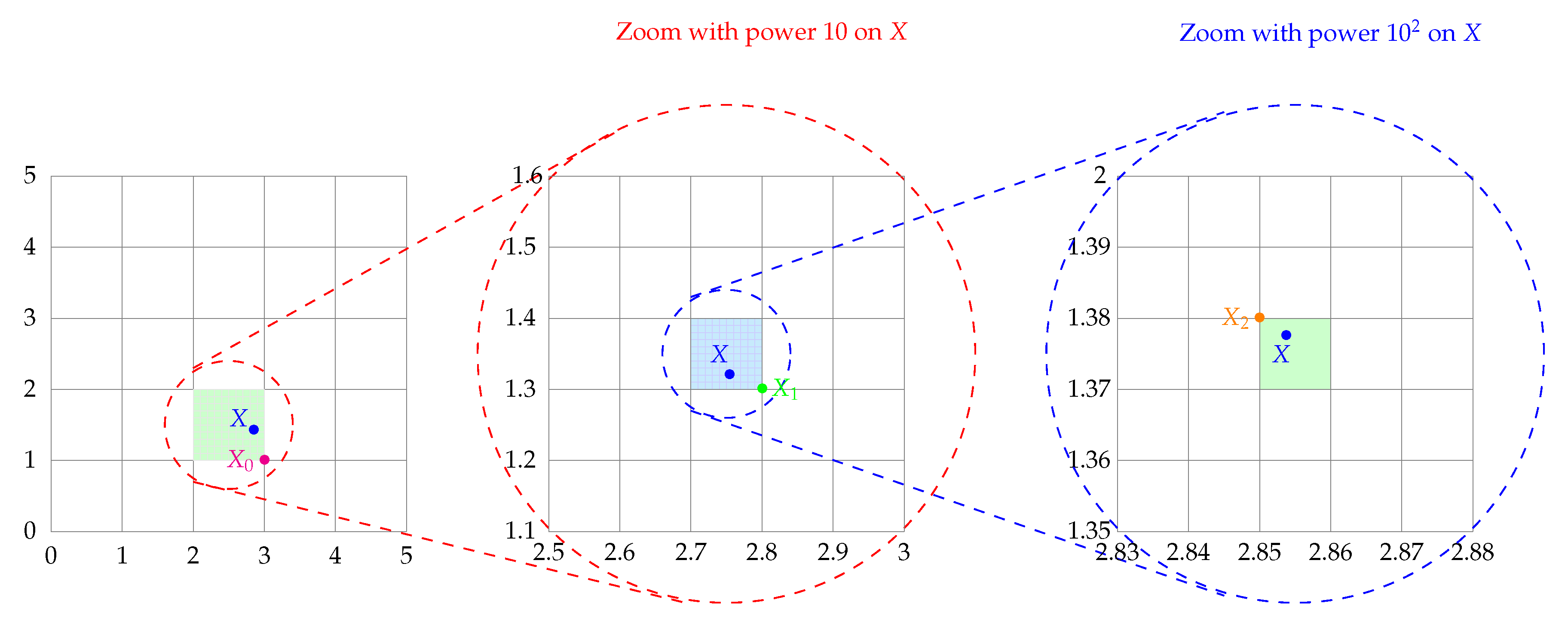
The proposed CFS procedure aims to speed up the intensification process and refines the accuracy of the search. Indeed, suppose that the solution X obtained at the end of $CGS/CLS$ search processes is close to the global optimum $X_o$ with precision ${10}^{-p}$, $p\in IN$. That can be formulated as:

$$X=X_o+\epsilon ,\parallel \epsilon \parallel <{10}^{-p}$$

(24)

Then the challenge is how to go beyond the accuracy ${10}^{-p}$?

One can observe that the distance $\epsilon$ can be interpreted as a parasitic signal of the solution, which is enough to filter in a suitable way to reach the global optimum, or it corresponds to the distance to which is the global optimum of its approximate solution. Thus, one solution is to conducts a search in a local area in which the radius adapts to the distance $\epsilon =X-X_o,$ component by component.

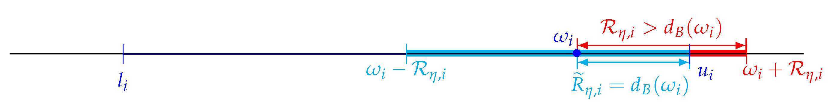
However, in practice, the global optimum is not known a priori. To overcome this difficulty, as we know that, as the search process proceeds the resulting solution X is supposed to be close enough to the global optimum, one solution is to consider instead of the relation (24) the difference between the current solution X and its decimals fractional parts of order $\eta$, $(\eta \in IN)$:

$${\epsilon }_{\eta }=|X-X_{\eta }|$$

where $X_{\eta }$ is the fractional of order $\eta ,$ i.e., the closest point of X to the precision ${10}^{-\eta }$ formalised as: $X_{\eta }={10}^{-\eta }round\left({10}^{\eta }X\right)$ (see Figure 10).

Furthermore, we propose to add a stochastic component in the round process in order to perturb a potential local optima. Indeed, we consider the stochastic round ${[.]}_{{}_{st}}$ defined by:

$${\left[X\right]}_{st}=\left\{\begin{array}{cc}round\left(X\right)+P,\hfill & ifmod(k,2)=0\hfill \\ round\left(X\right),\hfill & {\displaystyle otherwise}\hfill \end{array}\right.$$

(25)

where $P\sim U{(-1,1)}^d$ is a stochastic perturbation operated on X alternatively through The Tornado cycles. This way, the new formulation of the $\eta -$error of X is given by:

$${\tilde{\epsilon }}_{\eta }\left(X\right)=|X-{10}^{-\eta }{\left[{10}^{\eta }X\right]}_{{}_{st}}\left)\right|$$

(26)

The structure of the chaotic fine search CFS is similar to the CLS local chaotic search. Indeed, it proceeds by levelling approach creating $N_f$ levels, except the fact that the local area of level $\eta$ is defined by its radius ${\mathcal{R}}_{\eta }$ based on the $\eta -$error $\eta$ and given by:

$${\mathcal{R}}_{\eta }=\frac{1}{1+{\eta }^2}\widetilde{{\epsilon }_{\eta }},\eta \in \left[[0,N_f-1]\right]$$

(27)

This way, the local area search in CFS is carried out in a narrow domain that allow a focus on the current solution adapted coordinate by coordinate unlike the uniform local search in CLS as illustrated in Figure 11. The modified radius $\widetilde{R_{\eta }}$ is formulated as follows:

$$\widetilde{R_{\eta }}=\left\{\begin{array}{cc}s\times R·{\tilde{\epsilon }}_{\eta },\hfill & ifr>0.5\hfill \\ T·R·{\tilde{\epsilon }}_{\eta },\hfill & {\displaystyle otherwise}\hfill \end{array}\right.$$

(28)

where $r,s\sim U(0,1)$ and $T\sim U{(0,1)}^d$.

The design of the radius ${\mathcal{R}}_{\eta }$ allows to zoom at an exponential rate of decimal over the levels. Indeed, we have:

$$\parallel {\mathcal{R}}_{\eta }\parallel ⩽\parallel \widetilde{{\epsilon }_{\eta }}\parallel .\mathcal{R}<{10}^{-\eta }\times \mathcal{R}$$

(29)

As a consequence, the CFS provides an ultra fast exploitation of the neighborhood of the current solution and allows in principle the refinement of the optimum with a good precision.

The Fine Chaotic Search (CFS) is described in Algorithm 4 and the Tornado algorithm is detailed in Algorithm 5:

Algorithm 4 Chaotic Fine Search (CFS).

1: Input: $\mathit{f},\mathit{\omega },\mathit{L},\mathit{U},\mathit{Z},{\mathit{N}}_{\mathit{f}},{\mathit{N}}_{\mathit{p}}$ 2: Output: $X_l$: the best solution among local chaotic points 3: $\mathcal{R}=\frac{1}{2}(U-L);$ 4: $X=\omega ;$ 5: $X_l=\omega ;Y=f\left(\omega \right);$ 6: for$\eta =0$  to $N_l-1$ do 7:  Compute the $\eta -$error $\widetilde{{\epsilon }_{\eta }}$ and then evaluate ${\tilde{R}}_{\eta }$ using Equations (27)−(29) 8:  Generate two symmetrical chaotic variables $X_1$,  $X_2$ according to (23) 9:  for  $i=1$  to  2 10:    Choose randomly p in $\{1,\cdots ,n\}$ and decompose $X_i$ using (19) 11:    Generate $N_p$ symmetrical points $X_{i,j}$ according to (20) 12:    for $j=1$  à  $N_p$ 13:           if   $Y>f\left(X_{i,j}\right)$   then 14:                $X_l=X_{i,j};Y=f\left(X_{i,j}\right);$ 15:           end if 16:    end for 17:   end for 18: end for

Algorithm 5 Tornado Pseudo-Code.

1: Given:$f,L,U,Z,M,M_l,N_c,N_l,N_f,N_p$ 2: Output:$X,Y$ 3: $k=1;Y=+\infty ;$ 4: while    $k⩽M$    do 5:     $X_c=\mathbf{CGS}(f,L,U,Z_k,N_c)$ 6:     if   $Y>f\left(X_c\right)$    then 7:          $X=X_c;Y=f\left(X_c\right);$ 8:     end if 9:      $s=1;$ 10:     while $s⩽M_l$    do 11:          $X_l=\mathbf{CLS}(f,X,L,U,Z_{s+k},N_l,N_p)$ 12:          if    $Y>f\left(X_l\right)$    do 13:              $X=X_l;Y=f\left(X_l\right);$ 14:          end if 15:          $X_f=\mathbf{CFS}(f,X,L,U,Z_{s+k},N_f,N_p)$ 16:          if    $Y>f\left(X_l\right)$    do 17:              $X=X_f;Y=f\left(X_f\right);$ 18:          end if 19:          $s=s+1;$ 20:     end while 21:     $k=k+1;$ 22: end while

3. Scalarization-Based Chaotic Search

3.1. Tchebychev Scalarization Approaches

The aggregation (or weighted) method is one of the most popular scalarization method for the generation of Pareto optimal solutions. It consists in using an aggregation function to transform a $MOP$ into a single objective problem $\left(MO{P}_{\lambda }\right)$ by combining the various objective functions $f_i$ into a single objective function f generally in a linear way.

The first proposed scalarization approach (Multi-Objective Fractal Decomposition Algorithm Scalarization) uses the Tcheybycheff function [10,25]. It introduces the concept of ideal point or reference point $z_i^{*}$ as follows:

$$\begin{array}{ccccc}\hfill Minimize& \hfill {\displaystyle \underset{i=1,\dots ,k}{max}}& \multicolumn{3}{c}{\left[{\omega }_i(f_i\left(x\right)-z_i^{*})\right]}\\ \hfill \mathrm{Subject}\mathrm{to}& \hfill x\in \mathit{X}\end{array}$$

(30)

where $z^{*}$ = ($z_1^{*},\dots ,z_k^{*}$) is the reference point, and $\omega =({\omega }_1,\dots ,{\omega }_k)$ is the weight vector.

There have been numerous studies of decomposition approaches to use different types of reference points for providing evolutionary search directions. According to the position of reference point relative to the true PF in the objective space, we consider here three Tchebychev approaches:

• The Standard Tchebychev approach (TS) that consider the utopian point as the reference point.
• The modified Tchebychev variant (TM) that consider multiple utopian reference points instead of just one reference point [26] (see Figure 12).
• The augmented Tchebychev variant (AT) which is defined by the augmented Tchebychev function defined as [27]:

  $$\begin{array}{ccccc}\hfill Minimize& \hfill {\displaystyle \underset{i=1,\dots ,k}{max}}& \multicolumn{3}{c}{\left[{\omega }_i(f_i\left(x\right)-z_i^{*})\right]+\rho {\displaystyle \sum _{i=1}^m}{\omega }_i|z_i^{*}-f_i\left(x\right)|}\\ \hfill \mathrm{Subject}\mathrm{to}& \hfill x\in \mathit{X}\end{array}$$

  (31)

3.2. X-Tornado Algorithm

By using N different weight vectors $\omega$, we solves N different problems using the chaotic Tornado approach, each generating one solution composing the final Pareto Front (PF). One of the downsides of using scalarization methods is that the number of solutions composing the PF found by the algorithm will be, at most, the same as the number of different weight vectors N. In certain cases, if two or more weight vectors $\omega$ are too close, the algorithm might find the same solution.

4. Computational Experiments

The proposed algorithm X-Tornado is implemented on Matlab. The computing platform used consists of an Intel(R) Core(TM) i3 4005U CPU 1:70 GHz with 4 GB RAM.

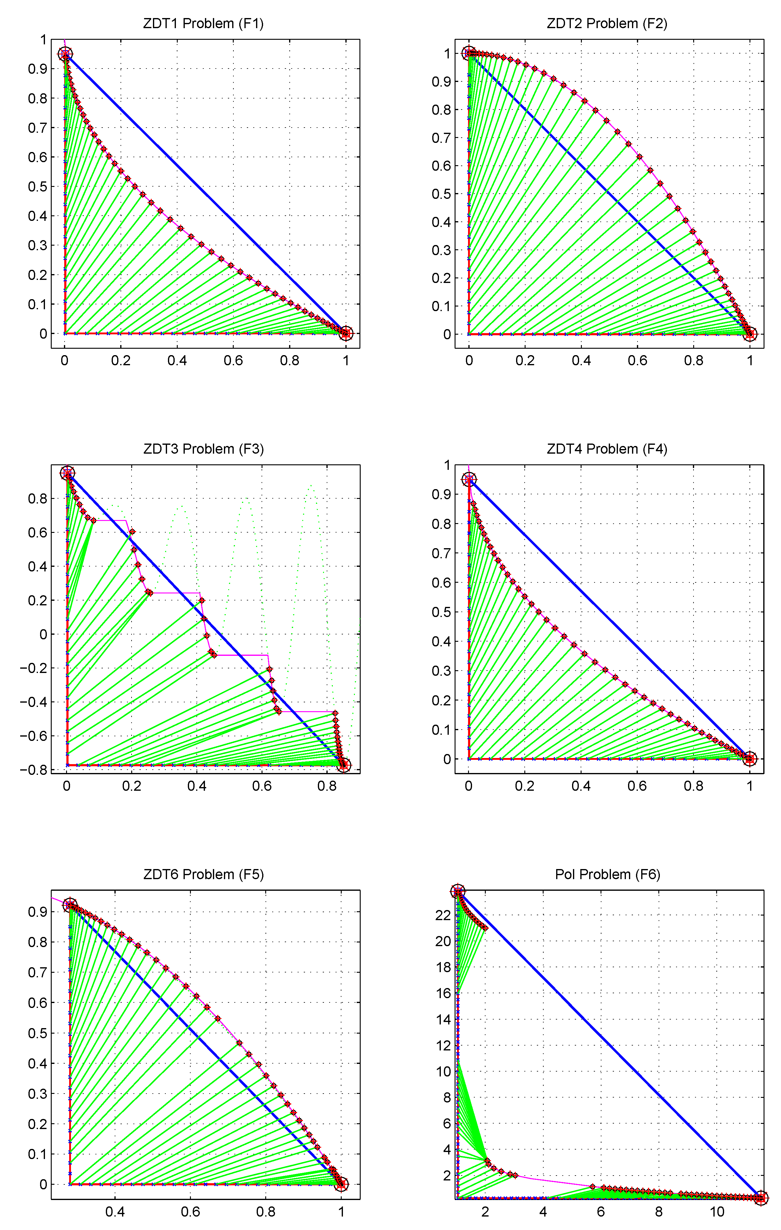
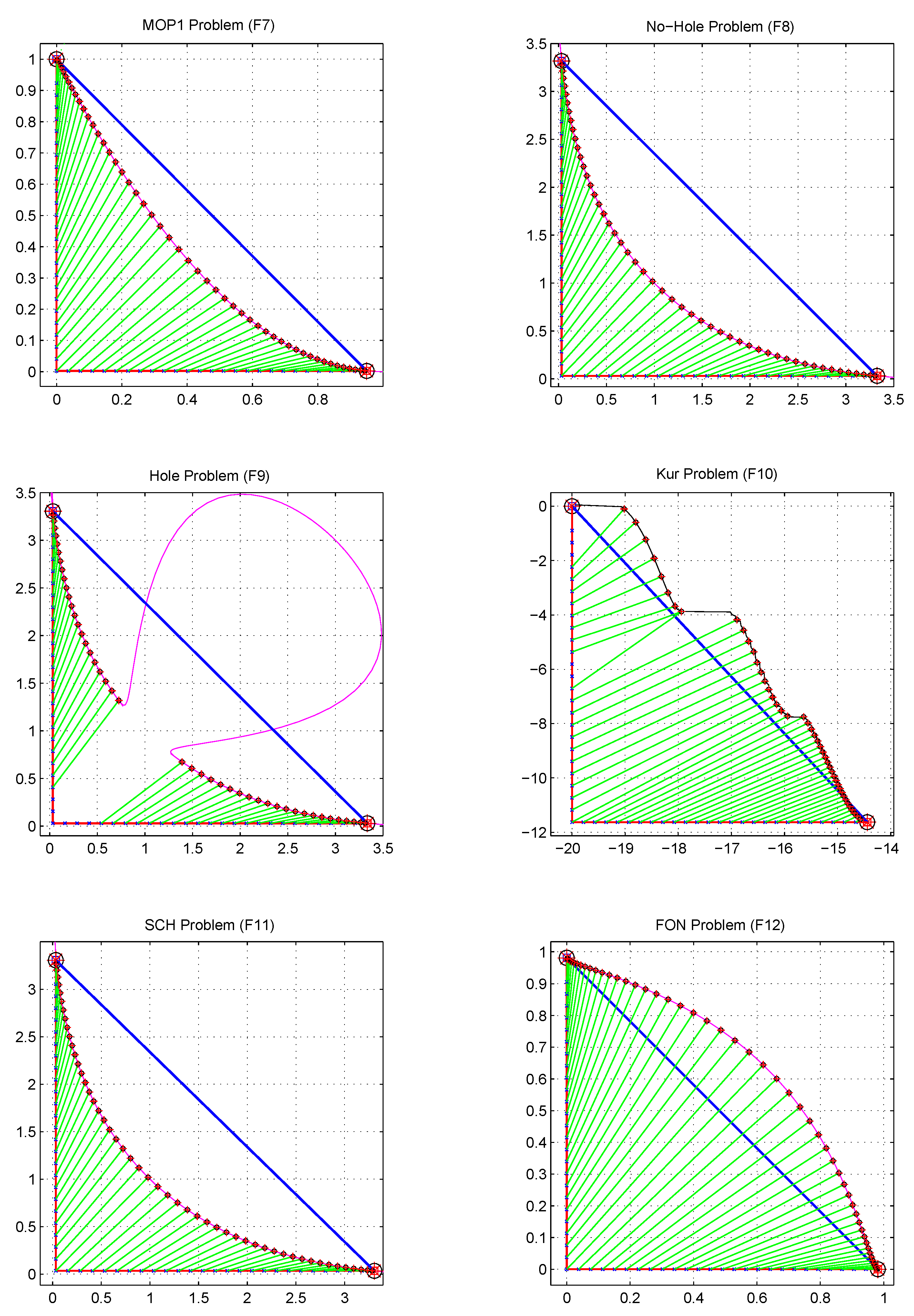
4.1. Test Problems

In order to evaluate the performance of the proposed X-Tornado algorithm, 14 test problems are selected from the literature. These functions will test the proposed algorithm’s performance in the different characteristics of the Pareto front: convexity, concavity, discreteness, non uniformity, and multimodality. For instance, the test problems KUR and ZDT3 have disconnected Pareto fronts; ZDT4 has too many local optimal Pareto solutions, whereas ZDT6 has non convex Pareto optimal front with low density of solutions near Pareto front. The test problems and their properties are shown in

Table 1. Benchmark Problems used in our experiments.

Problem	Name	n	Bounds	Objective Functions	Comments
ine $F_1$	$ZDT1$	30	${[0,1]}^n$	$f_1\left(x\right)=x_1$; $f_2\left(x\right)=g\left(x\right)(1-\sqrt{x_1/g\left(x\right)})$	Convex
				$g\left(x\right)=1+\frac{9}{n-1}{\displaystyle \sum _{i=2}^n}{x}_i$
$F_2$	$ZDT2$	30	${[0,1]}^n$	$f_1\left(x\right)=x_1$; $f_2\left(x\right)=g\left(x\right)(1-{(x_1/g\left(x\right))}^2)$	Non Convex
				$g\left(x\right)=1+\frac{9}{n-1}{\displaystyle \sum _{i=2}^n}{x}_i$
$F_3$	$ZDT3$	30	${[0,1]}^n$	$f_1\left(x\right)=x_1$; $f_2\left(x\right)=g\left(x\right)(1-\sqrt{x_1/g\left(x\right)}-(x_1/g\left(x\right))sin\left(10\pi x_1\right)$	Convex
				$g\left(x\right)=1+\frac{9}{n-1}{\displaystyle \sum _{i=2}^n}{x}_i$
$F_4$	$ZDT4$	30	${[0,1]}^n$	$f_1\left(x\right)=x_1$; $f_2\left(x\right)=g\left(x\right)(1-\sqrt{x_1/g\left(x\right)})$	Convex
				$g\left(x\right)=1+10(n-1){\displaystyle \sum _{i=2}^n}{x}_i^2-10cos\left(4\pi x_i\right)$
$F_5$	$ZDT6$	30	${[0,1]}^n$	$f_1\left(x\right)=1-exp\left(4x_1\right){sin}^6\left(6\pi x_1\right))$; $f_2\left(x\right)=g\left(x\right)(1-\sqrt{x_1/g\left(x\right)})$	Convex
				$g\left(x\right)=1+9{\left[\frac{1}{n-1}{\displaystyle \sum _{i=2}^n}{x}_i\right]}^{0.25}$
$F_6$	$POL$	2	${[-\pi ,\pi ]}^2$	$f_1\left(x\right)=1+{(A_1-B_1)}^2+{(A_2-B_2)}^2$; $f_2\left(x\right)={(x_1+3)}^2+{(x_2+1)}^2$	Convex
				$A_1=0.5sin\left(1\right)-2cos\left(1\right)+sin\left(2\right)-1.5cos\left(2\right)$
				$A_2=1.5sin\left(1\right)-cos\left(1\right)+2sin\left(2\right)-0.5cos\left(2\right)$
				$B_1=0.5sin\left(x_1\right)-2cos\left(x_1\right)+sin\left(x_2\right)-1.5cos\left(x_2\right)$
				$B_2=1.5sin\left(x_1\right)-cos\left(x_1\right)+2sin\left(x_2\right)-0.5cos\left(x_2\right)$
$F_7$	$MOP1$	1	$[-2,2]$	$f_1\left(x\right)=-x{\mathbf{1}}_{[-2,1]}\left(x\right)+(x-2){\mathbf{1}}_{]1,3]}\left(x\right)+(4-x){\mathbf{1}}_{]3,4]}\left(x\right)$	Non Convex
				$+(x-4){\mathbf{1}}_{]4,5]}\left(x\right);f_2\left(x\right)={(x-5)}^2$
$F_8$	$No$-$Hole$	2	${[-1,1]}^2$	$f_1\left(x\right)={(t+1)}^2+a$; $f_2\left(x\right)={(t-1)}^2+a$	Convex
$F_9$	$Hole$	2	${[-1,1]}^2$	$f_1\left(x\right)={(t+1)}^2+a+bexp[-c{(t-d)}^2]$;	Non Convex
				$f_2\left(x\right)={(t-1)}^2+a+bexp[-c{(t+d)}^2]$
$F_{10}$	$KUR$	3	${[-5,5]}^3$	$f_1\left(x\right)={\displaystyle \sum _{i=2}^n}(-10exp(-0.2\sqrt{x_i^1+x_i^2}))$; $f_2\left(x\right)={\displaystyle \sum _{i=1}^n}{\left|x_i\right|}^{0.8}+5sin\left(x_i^3\right)$	Convex
$F_{11}$	$SCH$	1	$[-{10}^{+3},{10}^{+3}]$	$f_1\left(x\right)=x^2$; $f_2\left(x\right)={(x-2)}^2$	Convex
$F_{12}$	$FON$	3	${[-4,4]}^3$	$f_1\left(x\right)=1-exp(-{\displaystyle \sum _{i=1}^3}(x_i-\frac{1}{\sqrt{3}}))$; $f_2\left(x\right)=1-exp(-{\displaystyle \sum _{i=1}^3}(x_i+\frac{1}{\sqrt{3}}))$	Convex
$F_{13}$	$MUR$	2	$[0,10]\times$	$f_1\left(x\right)=2\sqrt{x_1}$; $f_2\left(x\right)=x_1(1-x_2)+5$	Non Convex
			$[-10,10]$
$F_{14}$	$MSC$	1	$[-2,2]$	$f_1\left(x\right)=exp(-x)+1.4exp(-x^2)$; $f_2\left(x\right)=exp\left(x\right)+1.4exp(-x^2)$	Non Convex

.

4.2. Parameters Setting

In X-Tornado, the parameters setting were set as follows:

• The number of CGS chaotic levels $\left(N_c\right)$: $N_c=5$.
• The number of CLS chaotic levels $\left(N_l\right)$: $N_l=5$.
• The number of CFS chaotic levels $\left(N_f\right)$: $N_f=10$.
• The number of CLS-CFS per cycle $\left(M_l\right)$: $M_l=100$.
• The number of subproblems resolved with the Tchebychev decomposition approach $\left(N_s\right)$: $N_s=50$.

4.3. Performances Measures

Due to the fact that the convergence to the Pareto optimal front and the maintenance of a diverse set of solutions are two different goals of the multi-objective optimization, two performance measures were adopted in this study: the generational distance ($GD$) to evaluate the convergence, and the Spacing (S) to evaluate the diversity and cardinality.

• The convergence metric $\left(GD\right)$ measure the extent of convergence to the true Pareto front. It is defined as:

  $$GD={\displaystyle \frac{1}{N}}{\displaystyle \sum _{i=1}^N}{d}_i,$$

  (32)

  where N is the number of solutions found and $d_i$ is the Euclidean distance between each solution and its nearest point in the true Pareto front. The lower value of GD, the better convergence of the Pareto front to the real one.
• The Spacing metric S indicates how the solutions of an obtained Pareto front are spaced with respect to each other. It is defined as:

  $$S=\sqrt{{\displaystyle \frac{1}{N}}{\displaystyle \sum _{i=1}^N}{(d_i-\overline{d})}^2}$$

  (33)

4.4. Impact of the Tchebychev Scalarization Strategies

By adopting the three Tchebychev we have tested three X-Tornado variants as follows:

• X-Tornado-TS: denotes X-Torando with Standard Tchebychev approach.
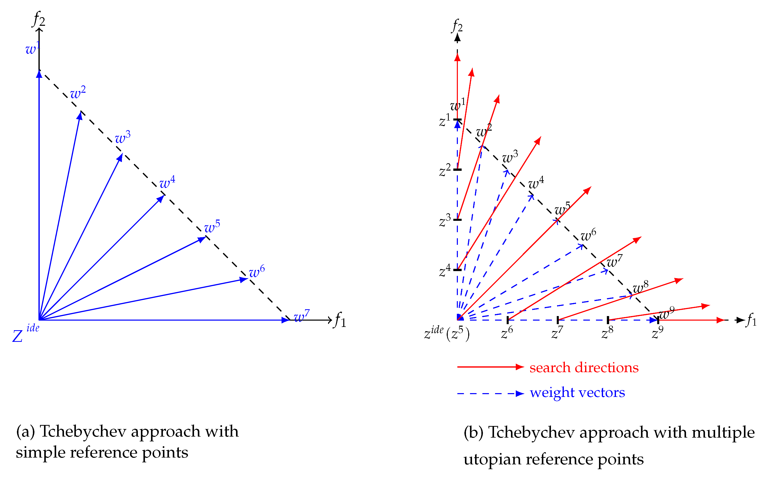
• X-Tornado-TM: denotes X-Torando with Tchebychev variant involving multiple utopian reference points instead of just one reference point.
• X-Tornado-ATS: denotes X-Torando with augmented Tchebychev approach.

The computational results in term of $(GD$, S) for 300000 function evaluations are shown in

Table 2. The Generationnal distance metric result for the three versions of X-Tornado on the 14 selected problems.

	XTornado-TS		XTornado-TM		XTornado-ATS
Problem	Mean	Std	Mean	Std	Mean	Std
ine $F_1$	$1.27\times {10}^{-3}$	$4.50\times {10}^{-7}$	$2.38\times {10}^{-3}$	$7.10\times {10}^{-7}$	$1.27\times {10}^{-3}$	$1.70\times {10}^{-6}$
$F_2$	$5.24\times {10}^{-4}$	$6.09\times {10}^{-4}$	$6.61\times {10}^{-4}$	$4.42\times {10}^{-4}$	$8.68\times {10}^{-4}$	$1.08\times {10}^{-3}$
$F_3$	$2.91\times {10}^{-3}$	$1.24\times {10}^{-4}$	$2.45\times {10}^{-3}$	$1.68\times {10}^{-4}$	$2.52\times {10}^{-3}$	$5.36\times {10}^{-4}$
$F_4$	$1.51\times {10}^{-3}$	$3.81\times {10}^{-4}$	$1.72\times {10}^{-3}$	$3.61\times {10}^{-4}$	$1.34\times {10}^{-3}$	$1.88\times {10}^{-6}$
$F_5$	$5.76\times {10}^{-3}$	$2.23\times {10}^{-3}$	$3.88\times {10}^{-3}$	$1.97\times {10}^{-3}$	$9.57\times {10}^{-4}$	$1.26\times {10}^{-4}$
$F_6$	$1.45\times {10}^{-3}$	$1.08\times {10}^{-4}$	$1.39\times {10}^{-3}$	$3.41\times {10}^{-5}$	$1.40\times {10}^{-3}$	$8.18\times {10}^{-5}$
$F_7$	$1.27\times {10}^{-3}$	$1.13\times {10}^{-6}$	$2.38\times {10}^{-3}$	$5.41\times {10}^{-7}$	$1.27\times {10}^{-3}$	$1.62\times {10}^{-6}$
$F_8$	$2.38\times {10}^{-3}$	$1.01\times {10}^{-4}$	$2.38\times {10}^{-3}$	$1.23\times {10}^{-6}$	$2.50\times {10}^{-3}$	$2.41\times {10}^{-4}$
$F_9$	$3.06\times {10}^{-3}$	$1.32\times {10}^{-4}$	$2.16\times {10}^{-3}$	$4.11\times {10}^{-4}$	$2.67\times {10}^{-3}$	$1.87\times {10}^{-4}$
$F_{10}$	$5.95\times {10}^{-4}$	$1.17\times {10}^{-5}$	$6.41\times {10}^{-4}$	$5.50\times {10}^{-6}$	$5.86\times {10}^{-4}$	$6.20\times {10}^{-6}$
$F_{11}$	$2.07\times {10}^{-3}$	$4.15\times {10}^{-10}$	$2.38\times {10}^{-3}$	$4.30\times {10}^{-10}$	$2.07\times {10}^{-3}$	$1.09\times {10}^{-9}$
$F_{12}$	$9.76\times {10}^{-4}$	$9.33\times {10}^{-7}$	$8.42\times {10}^{-4}$	$1.43\times {10}^{-6}$	$9.76\times {10}^{-4}$	$5.03\times {10}^{-7}$
$F_{13}$	$8.76\times {10}^{-4}$	$8.60\times {10}^{-11}$	$7.80\times {10}^{-4}$	$7.50\times {10}^{-13}$	$8.76\times {10}^{-4}$	$2.65\times {10}^{-13}$
$F_{14}$	$4.24\times {10}^{-4}$	$1.37\times {10}^{-11}$	$5.66\times {10}^{-4}$	$1.02\times {10}^{-11}$	$4.24\times {10}^{-4}$	$3.47\times {10}^{-11}$

TS: Standard Tchebytcheff, TM: Tchebytcheff with multiple references points, ATS: Augmented Tchebytcheff.

and

Table 3. Results of the Spacing metric $\left(S\right)$ for the three versions of X-Tornado on the 14 selected problems.

	XTornado-TS		XTornado-TM		XTornado-ATS
Problem	Mean	Std	Mean	Std	Mean	Std
ine $F_1$	$1.42\times {10}^{-2}$	$3.06\times {10}^{-5}$	$1.14\times {10}^{-2}$	$2.05\times {10}^{-7}$	$1.43\times {10}^{-2}$	$3.71\times {10}^{-6}$
$F_2$	$6.74\times {10}^{-3}$	$8.33\times {10}^{-3}$	$1.61\times {10}^{-2}$	$1.08\times {10}^{-2}$	$1.88\times {10}^{-2}$	$2.89\times {10}^{-2}$
$F_3$	$5.64\times {10}^{-2}$	$1.72\times {10}^{-3}$	$4.69\times {10}^{-2}$	$2.31\times {10}^{-3}$	$5.61\times {10}^{-2}$	$7.01\times {10}^{-3}$
$F_4$	$3.90\times {10}^{-2}$	$4.27\times {10}^{-3}$	$1.45\times {10}^{-2}$	$2.25\times {10}^{-3}$	$4.16\times {10}^{-2}$	$3.39\times {10}^{-3}$
$F_5$	$7.47\times {10}^{-2}$	$2.20\times {10}^{-2}$	$6.46\times {10}^{-2}$	$1.80\times {10}^{-2}$	$1.53\times {10}^{-2}$	$3.43\times {10}^{-3}$
$F_6$	$1.43\times {10}^{-2}$	$2.36\times {10}^{-7}$	$1.14\times {10}^{-2}$	$3.23\times {10}^{-6}$	$1.43\times {10}^{-2}$	$9.73\times {10}^{-7}$
$F_7$	$1.43\times {10}^{-2}$	$2.01\times {10}^{-6}$	$1.14\times {10}^{-2}$	$2.80\times {10}^{-6}$	$1.43\times {10}^{-2}$	$3.45\times {10}^{-6}$
$F_8$	$1.01\times {10}^{-2}$	$4.76\times {10}^{-4}$	$2.44\times {10}^{-2}$	$3.36\times {10}^{-3}$	$9.93\times {10}^{-2}$	$2.92\times {10}^{-2}$
$F_9$	$5.95\times {10}^{-2}$	$5.04\times {10}^{-3}$	$4.94\times {10}^{-2}$	$5.23\times {10}^{-3}$	$5.68\times {10}^{-2}$	$3.55\times {10}^{-3}$
$F_{10}$	$2.70\times {10}^{-1}$	$1.68\times {10}^{-2}$	$3.15\times {10}^{-1}$	$2.61\times {10}^{-2}$	$2.57\times {10}^{-1}$	$1.49\times {10}^{-2}$
$F_{11}$	$9.03\times {10}^{-2}$	$1.28\times {10}^{-8}$	$1.14\times {10}^{-2}$	$1.52\times {10}^{-6}$	$9.03\times {10}^{-2}$	$2.75\times {10}^{-8}$
$F_{12}$	$4.67\times {10}^{-3}$	$8.65\times {10}^{-7}$	$1.86\times {10}^{-2}$	$4.59\times {10}^{-7}$	$4.67\times {10}^{-3}$	$2.88\times {10}^{-7}$
$F_{13}$	$1.48\times {10}^{-2}$	$1.15\times {10}^{-12}$	$4.46\times {10}^{-2}$	$1.43\times {10}^{-11}$	$1.48\times {10}^{-2}$	$3.34\times {10}^{-12}$
$F_{14}$	$1.44\times {10}^{-1}$	$1.14\times {10}^{-9}$	$4.57\times {10}^{-2}$	$8.71\times {10}^{-11}$	$1.44\times {10}^{-1}$	$2.13\times {10}^{-9}$

TS: Standard Tchebytcheff, TM: Tchebytcheff with multiple references points, ATS: Augmented Tchebytcheff.

respectively, according to the three variants of X-Tornado.

The analysis of the results obtained for the 14 selected problems show that X-Tornado-TM achieves the best performance in term of the two considered metrics $GD$ and S. Indeed, in term of convergence X-Tornado-TM wins the competition on 6 problems, X-Tornado-TS wins on 5 problems whereas X-Tornado-ATS wins on only 3 problems. In term of spacing metric, X-Tornado-TM releases clearly the best performance by winning the competition on $8/14$ whereas X-Tornado-TS and X-Tornado-ATS win both only on three problems.

Based on this performance analysis, X-Tornado-TM variant seems to be the most promising one and therefore, in the next section we will compare its performance against some state-of the-art evolutionary algorithms. Moreover, it will be designed as X-Tornado for sake of simplicity.

4.5. Comparison with Some State-Of The-Art Evolutionary Algorithms

In this section, we choose three well-known multiobjective evolutionary algorithms NSGA-II, PESA-II, and MOEA/D (MATLAB implementation obtained for the yarpiz library available at www.yarpiz.com.). The Tchebychev function in MOEA/D was selected as the scalarizing function and the neighborhood size was specified as $15\%$ of the population size. The population size in the three algorithms was set to 100, The size of the archive was set to 50 in PESA-II and MOEA/D.

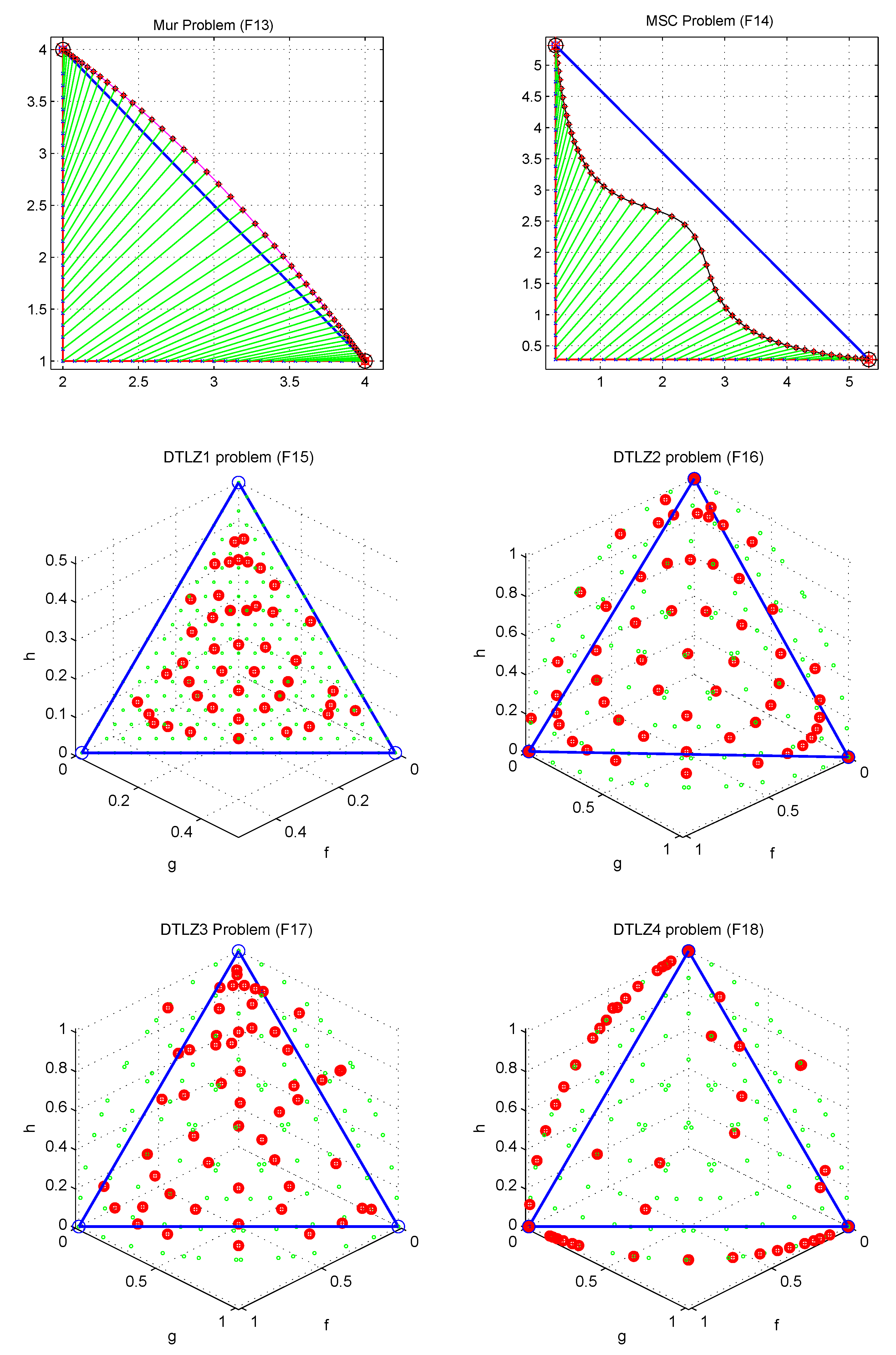
Besides the 14 bi-objective considered problems in the previous section, 4 additional 3d objective problems will be also tested, which are DTLZ1, DTLZ2, DTLZ3, DTLZ4. However, note that, as the TM decomposition is not suitable in the 3d cases, those 3d problems will be tested with X-Tornado-TS variant.

The computational results using the performance indicators $(GD$ and S for 300000 function evaluations are shown in

Table 4. The Generational distance metric $\left(GD\right)$ comparison result for the for algorithms on the 14 selected problems.

	Nsga2		Pesa2		Moead		Xtornado-TM
Fct	Mean	Std	Mean	Std	Mean	Std	Mean	Std
ine $F_1$	$6.69\times {10}^{-3}$	$1.50\times {10}^{-3}$	$5.87\times {10}^{-2}$	$1.22\times {10}^{-2}$	$2.74\times {10}^{-2}$	$2.49\times {10}^{-2}$	$\mathbf{2.38}\times {\mathbf{10}}^{-\mathbf{3}}$	$\mathbf{7.10}\times {\mathbf{10}}^{-\mathbf{7}}$
$F_2$	$6.56\times {10}^{-3}$	$1.43\times {10}^{-3}$	$8.62\times {10}^{-2}$	$5.97\times {10}^{-3}$	$2.48\times {10}^{-1}$	$1.04\times {10}^{-1}$	$\mathbf{6.61}\times {\mathbf{10}}^{-\mathbf{4}}$	$\mathbf{4.42}\times {\mathbf{10}}^{-\mathbf{4}}$
$F_3$	$1.15\times {10}^{-2}$	$4.57\times {10}^{-3}$	$4.20\times {10}^{-2}$	$3.75\times {10}^{-3}$	$3.27\times {10}^{-2}$	$1.71\times {10}^{-2}$	$\mathbf{2.45}\times {\mathbf{10}}^{-\mathbf{3}}$	$\mathbf{1.68}\times {\mathbf{10}}^{-\mathbf{4}}$
$F_4$	$8.63\times {10}^{-2}$	$8.00\times {10}^{-2}$	$1.07\times {10}^{+1}$	$2.87\times {10}^{-1}$	$8.49\times {10}^{+0}$	$2.04\times {10}^{+0}$	$\mathbf{1.72}\times {\mathbf{10}}^{-\mathbf{3}}$	$\mathbf{3.61}\times {\mathbf{10}}^{-\mathbf{4}}$
$F_5$	$1.54\times {10}^{-2}$	$3.14\times {10}^{-2}$	$4.37\times {10}^{-1}$	$8.26\times {10}^{-3}$	$6.62\times {10}^{-1}$	$1.78\times {10}^{-1}$	$\mathbf{3.88}\times {\mathbf{10}}^{-\mathbf{3}}$	$\mathbf{1.97}\times {\mathbf{10}}^{-\mathbf{3}}$
$F_6$	$\mathbf{9.73}\times {\mathbf{10}}^{-\mathbf{4}}$	$\mathbf{4.76}\times {\mathbf{10}}^{-\mathbf{5}}$	$8.83\times {10}^{-2}$	$2.49\times {10}^{-2}$	$1.57\times {10}^{-3}$	$1.31\times {10}^{-3}$	$1.39\times {10}^{-3}$	$3.41\times {10}^{-5}$
$F_7$	$\mathbf{6.96}\times {\mathbf{10}}^{-\mathbf{5}}$	$\mathbf{6.44}\times {\mathbf{10}}^{-\mathbf{6}}$	$9.26\times {10}^{+1}$	$1.00\times {10}^{+1}$	$5.66\times {10}^{-4}$	$9.35\times {10}^{-4}$	$2.38\times {10}^{-3}$	$5.41\times {10}^{-7}$
$F_8$	$\mathbf{1.74}\times {\mathbf{10}}^{-\mathbf{3}}$	$\mathbf{2.52}\times {\mathbf{10}}^{-\mathbf{5}}$	$6.45\times {10}^{-2}$	$5.93\times {10}^{-3}$	$1.30\times {10}^{-3}$	$2.12\times {10}^{-4}$	$2.38\times {10}^{-3}$	$1.23\times {10}^{-6}$
$F_9$	$4.08\times {10}^{-2}$	$9.28\times {10}^{-3}$	$3.75\times {10}^{-2}$	$4.12\times {10}^{-3}$	$1.88\times {10}^{-2}$	$4.04\times {10}^{-3}$	$\mathbf{2.16}\times {\mathbf{10}}^{-\mathbf{3}}$	$\mathbf{4.11}\times {\mathbf{10}}^{-\mathbf{4}}$
$F_{10}$	$7.38\times {10}^{-4}$	$8.84\times {10}^{-5}$	$1.78\times {10}^{-1}$	$1.08\times {10}^{-2}$	$1.13\times {10}^{-2}$	$1.26\times {10}^{-2}$	$\mathbf{6.41}\times {\mathbf{10}}^{-\mathbf{4}}$	$\mathbf{5.50}\times {\mathbf{10}}^{-\mathbf{6}}$
$F_{11}$	$4.51\times {10}^{-3}$	$6.32\times {10}^{-4}$	$1.82\times {10}^{+9}$	$1.89\times {10}^{+8}$	$4.59\times {10}^{+0}$	$1.01\times {10}^{+1}$	$\mathbf{2.38}\times {\mathbf{10}}^{-\mathbf{3}}$	$\mathbf{4.30}\times {\mathbf{10}}^{-\mathbf{10}}$
$F_{12}$	$1.05\times {10}^{-3}$	$1.27\times {10}^{-4}$	$3.23\times {10}^{-2}$	$1.03\times {10}^{-3}$	$1.27\times {10}^{-3}$	$4.30\times {10}^{-4}$	$\mathbf{8.42}\times {\mathbf{10}}^{-\mathbf{4}}$	$\mathbf{1.43}\times {\mathbf{10}}^{-\mathbf{6}}$
$F_{13}$	$8.29\times {10}^{-4}$	$9.40\times {10}^{-5}$	$6.28\times {10}^{-3}$	$1.81\times {10}^{-3}$	$2.04\times {10}^{-3}$	$3.16\times {10}^{-3}$	$\mathbf{7.80}\times {\mathbf{10}}^{-\mathbf{4}}$	$\mathbf{7.50}\times {\mathbf{10}}^{-\mathbf{13}}$
$F_{14}$	$6.05\times {10}^{-4}$	$6.94\times {10}^{-5}$	$2.98\times {10}^{-4}$	$1.79\times {10}^{-4}$	$3.66\times {10}^{-4}$	$8.88\times {10}^{-5}$	$\mathbf{5.66}\times {\mathbf{10}}^{-\mathbf{4}}$	$\mathbf{1.02}\times {\mathbf{10}}^{-\mathbf{11}}$

and

Table 5. The Spacing metric $\left(S\right)$ comparison result for the four algorithms on the 14 selected problems.

	Nsga2		Pesa2		Moead		Xtornado-TM
Fct	Mean	Std	Mean	Std	Mean	Std	Mean	Std
ine $F_1$	$1.20\times {10}^{-2}$	$4.19\times {10}^{-3}$	$3.70\times {10}^{-1}$	$3.51\times {10}^{-2}$	$3.74\times {10}^{-2}$	$1.79\times {10}^{-2}$	$\mathbf{1.14}\times {\mathbf{10}}^{-\mathbf{2}}$	$\mathbf{2.05}\times {\mathbf{10}}^{-\mathbf{7}}$
$F_2$	$7.75\times {10}^{-3}$	$3.00\times {10}^{-3}$	$5.28\times {10}^{-1}$	$3.86\times {10}^{-2}$	$1.06\times {10}^{-1}$	$1.05\times {10}^{-1}$	$\mathbf{1.61}\times {\mathbf{10}}^{-\mathbf{2}}$	$\mathbf{1.08}\times {\mathbf{10}}^{-\mathbf{2}}$
$F_3$	$\mathbf{3.40}\times {\mathbf{10}}^{-\mathbf{2}}$	$\mathbf{7.73}\times {\mathbf{10}}^{-\mathbf{3}}$	$3.78\times {10}^{-1}$	$2.14\times {10}^{-2}$	$7.86\times {10}^{-2}$	$9.79\times {10}^{-3}$	$4.69\times {10}^{-2}$	$2.31\times {10}^{-3}$
$F_4$	$3.21\times {10}^{-1}$	$6.38\times {10}^{-1}$	$2.38\times {10}^{+1}$	$2.61\times {10}^{+0}$	$1.04\times {10}^{+0}$	$2.34\times {10}^{+0}$	$\mathbf{1.45}\times {\mathbf{10}}^{-\mathbf{2}}$	$\mathbf{2.25}\times {\mathbf{10}}^{-\mathbf{3}}$
$F_5$	$7.58\times {10}^{-2}$	$1.36\times {10}^{-1}$	$9.86\times {10}^{+0}$	$1.72\times {10}^{+0}$	$1.34\times {10}^{+0}$	$1.39\times {10}^{+0}$	$\mathbf{6.46}\times {\mathbf{10}}^{-\mathbf{2}}$	$\mathbf{1.80}\times {\mathbf{10}}^{-\mathbf{2}}$
$F_6$	$2.44\times {10}^{+0}$	$3.74\times {10}^{-3}$	$1.90\times {10}^{+0}$	$4.29\times {10}^{-1}$	$1.43\times {10}^{-1}$	$1.04\times {10}^{-1}$	$\mathbf{1.14}\times {\mathbf{10}}^{-\mathbf{2}}$	$\mathbf{2.17}\times {\mathbf{10}}^{-\mathbf{7}}$
$F_7$	$1.11\times {10}^{+0}$	$1.10\times {10}^{-3}$	$4.04\times {10}^{-1}$	$9.21\times {10}^{-2}$	$1.09\times {10}^{-1}$	$8.63\times {10}^{-3}$	$\mathbf{1.14}\times {\mathbf{10}}^{-\mathbf{2}}$	$\mathbf{2.80}\times {\mathbf{10}}^{-\mathbf{6}}$
$F_8$	$4.76\times {10}^{-2}$	$7.48\times {10}^{-3}$	$2.53\times {10}^{-1}$	$4.44\times {10}^{-2}$	$4.19\times {10}^{-1}$	$1.19\times {10}^{-1}$	$\mathbf{2.44}\times {\mathbf{10}}^{-\mathbf{2}}$	$\mathbf{3.36}\times {\mathbf{10}}^{-\mathbf{3}}$
$F_9$	$9.70\times {10}^{-2}$	$3.24\times {10}^{-3}$	$1.97\times {10}^{+0}$	$3.43\times {10}^{-1}$	$3.15\times {10}^{-1}$	$2.19\times {10}^{-1}$	$\mathbf{4.94}\times {\mathbf{10}}^{-\mathbf{2}}$	$\mathbf{5.23}\times {\mathbf{10}}^{-\mathbf{3}}$
$F_{10}$	$\mathbf{1.79}\times {\mathbf{10}}^{-\mathbf{1}}$	$\mathbf{1.11}\times {\mathbf{10}}^{-\mathbf{2}}$	$3.67\times {10}^{+2}$	$3.01\times {10}^{+1}$	$5.10\times {10}^{-1}$	$7.39\times {10}^{-1}$	$3.15\times {10}^{-1}$	$2.61\times {10}^{-2}$
$F_{11}$	$7.62\times {10}^{-2}$	$1.25\times {10}^{-2}$	$1.31\times {10}^{+0}$	$2.05\times {10}^{-1}$	$1.57\times {10}^{-1}$	$2.18\times {10}^{-2}$	$\mathbf{2.46}\times {\mathbf{10}}^{-\mathbf{2}}$	$\mathbf{1.57}\times {\mathbf{10}}^{-\mathbf{8}}$
$F_{12}$	$1.47\times {10}^{-2}$	$2.95\times {10}^{-3}$	$4.26\times {10}^{+0}$	$7.91\times {10}^{-1}$	$6.99\times {10}^{-1}$	$3.08\times {10}^{-1}$	$\mathbf{1.86}\times {\mathbf{10}}^{-\mathbf{2}}$	$\mathbf{4.59}\times {\mathbf{10}}^{-\mathbf{7}}$
$F_{13}$	$4.93\times {10}^{-2}$	$8.37\times {10}^{-3}$	$4.22\times {10}^{+4}$	$1.54\times {10}^{+3}$	$1.10\times {10}^{-1}$	$1.16\times {10}^{-1}$	$\mathbf{4.46}\times {\mathbf{10}}^{-\mathbf{2}}$	$\mathbf{1.43}\times {\mathbf{10}}^{-\mathbf{11}}$
$F_{14}$	$1.44\times {10}^{-1}$	$7.03\times {10}^{-3}$	$1.45\times {10}^{-1}$	$4.43\times {10}^{-2}$	$\mathbf{2.43}\times {\mathbf{10}}^{-\mathbf{2}}$	$\mathbf{3.54}\times {\mathbf{10}}^{-\mathbf{3}}$	$4.57\times {10}^{-2}$	$8.71\times {10}^{-11}$

respectively, according to all four algorithms: NSGA-II, PESA-II, MOEA-D, and X-Tornado. The mean and variance of simulation results in 10 independent experiments are depicted for each algorithm. The mean of the metrics reveals the average evolutionary performance and represents the optimization results in comparison with other algorithms. The variance of the metrics indicates the consistency of an algorithm. The best performance is represented by bold fonts.

By analysing the obtained results in Table 4, it is clear that the X-Tornado approach has the best performance in term of convergence to the front. Indeed the proposed X-Tornado obtains the lowest $GD$ metric value for twelve out of the 18 test problems and with small standard deviation in almost all problems. A low $GD$ metric value of an algorithm on a problem is significant for accuracy of the obtained Pareto front. That is to say, the proposed algorithm has a good accuracy and stability on the performance of these problems.

In Table 5 X-Tornado outperforms all other algorithms on the mean of the spacing metric in almost all test problems except in ZDT3, KUR, MSC and DTLZ4.

The next

Table 6. The Generational distance metric $\left(GD\right)$ comparison results for the for algorithms on the 8 selected problems.

	Nsga2		Pesa2		Moead		X-Tornado
Problem	Mean	Std	Mean	Std	Mean	Std	Mean	Std
ine $F_1$	$3.79\times {10}^{-3}$	$7.68\times {10}^{-4}$	$6.44\times {10}^{-2}$	$1.31\times {10}^{-2}$	$4.46\times {10}^{-3}$	$7.26\times {10}^{-3}$	$\mathbf{2.38}\times {\mathbf{10}}^{-\mathbf{3}}$	$\mathbf{7.10}\times {\mathbf{10}}^{-\mathbf{7}}$
$F_2$	$3.97\times {10}^{-3}$	$8.13\times {10}^{-4}$	$8.72\times {10}^{-2}$	$6.64\times {10}^{-3}$	$1.05\times {10}^{-1}$	$5.58\times {10}^{-2}$	$\mathbf{6.61}\times {\mathbf{10}}^{-\mathbf{4}}$	$\mathbf{4.42}\times {\mathbf{10}}^{-\mathbf{4}}$
$F_3$	$3.86\times {10}^{-3}$	$1.07\times {10}^{-3}$	$4.37\times {10}^{-2}$	$2.78\times {10}^{-3}$	$2.39\times {10}^{-2}$	$7.76\times {10}^{-3}$	$\mathbf{2.45}\times {\mathbf{10}}^{-\mathbf{3}}$	$\mathbf{1.68}\times {\mathbf{10}}^{-\mathbf{4}}$
$F_4$	$8.82\times {10}^{-2}$	$9.24\times {10}^{-2}$	$1.11\times {10}^{+1}$	$6.62\times {10}^{-1}$	$3.31\times {10}^{+0}$	$1.05\times {10}^{+0}$	$\mathbf{1.72}\times {\mathbf{10}}^{-\mathbf{3}}$	$\mathbf{3.61}\times {\mathbf{10}}^{-\mathbf{4}}$
$F_5$	$\mathbf{9.99}\times {\mathbf{10}}^{-\mathbf{4}}$	$\mathbf{2.52}\times {\mathbf{10}}^{-\mathbf{5}}$	$6.70\times {10}^{-2}$	0	$8.52\times {10}^{-4}$	$5.15\times {10}^{-5}$	$3.88\times {10}^{-3}$	$1.97\times {10}^{-3}$
$F_6$	$\mathbf{4.44}\times {\mathbf{10}}^{-\mathbf{4}}$	$\mathbf{3.45}\times {\mathbf{10}}^{-\mathbf{5}}$	$4.08\times {10}^{-1}$	0	$2.72\times {10}^{-1}$	$1.97\times {10}^{-1}$	$1.39\times {10}^{-3}$	$3.41\times {10}^{-5}$
$F_7$	$\mathbf{6.57}\times {\mathbf{10}}^{-\mathbf{4}}$	$\mathbf{2.38}\times {\mathbf{10}}^{-\mathbf{5}}$	$1.18\times {10}^{-1}$	0	$6.86\times {10}^{-3}$	$5.65\times {10}^{-3}$	$2.38\times {10}^{-3}$	$5.41\times {10}^{-7}$
$F_8$	$7.65\times {10}^{-3}$	$1.38\times {10}^{-2}$	$5.27\times {10}^{-2}$	0	$1.00\times {10}^{-2}$	$1.45\times {10}^{-3}$	$\mathbf{2.38}\times {\mathbf{10}}^{-\mathbf{3}}$	$\mathbf{1.23}\times {\mathbf{10}}^{-\mathbf{6}}$

and

Table 7. The Spacing metric $\left(S\right)$ comparison results for the four algorithms on the 8 selected problems.

	Nsga2		Pesa2		Moead		X-Tornado
Problem	Mean	Std	Mean	Std	Mean	Std	Mean	Std
ine $F_1$	$\mathbf{8.07}\times {\mathbf{10}}^{-\mathbf{3}}$	$\mathbf{2.61}\times {\mathbf{10}}^{-\mathbf{3}}$	$3.77\times {10}^{-1}$	$4.27\times {10}^{-2}$	$2.18\times {10}^{-2}$	$5.26\times {10}^{-3}$	$1.14\times {10}^{-2}$	$2.05\times {10}^{-7}$
$F_2$	$\mathbf{7.92}\times {\mathbf{10}}^{-\mathbf{3}}$	$\mathbf{2.86}\times {\mathbf{10}}^{-\mathbf{3}}$	$5.40\times {10}^{-1}$	$4.55\times {10}^{-2}$	$2.50\times {10}^{-2}$	$3.55\times {10}^{-3}$	$1.61\times {10}^{-2}$	$1.08\times {10}^{-2}$
$F_3$	$\mathbf{2.65}\times {\mathbf{10}}^{-\mathbf{2}}$	$\mathbf{2.40}\times {\mathbf{10}}^{-\mathbf{3}}$	$3.95\times {10}^{-1}$	$2.38\times {10}^{-2}$	$4.76\times {10}^{-2}$	$1.63\times {10}^{-2}$	$4.69\times {10}^{-2}$	$2.31\times {10}^{-3}$
$F_4$	$1.10\times {10}^{+0}$	$1.29\times {10}^{+0}$	$2.41\times {10}^{+1}$	$1.12\times {10}^{+0}$	$2.53\times {10}^{-1}$	$1.92\times {10}^{-1}$	$\mathbf{1.45}\times {\mathbf{10}}^{-\mathbf{2}}$	$\mathbf{2.25}\times {\mathbf{10}}^{-\mathbf{3}}$
$F_5$	$1.75\times {10}^{+0}$	$1.90\times {10}^{-3}$	$8.78\times {10}^{+0}$	0	$7.34\times {10}^{-1}$	$7.85\times {10}^{-1}$	$\mathbf{6.46}\times {\mathbf{10}}^{-\mathbf{2}}$	$\mathbf{1.80}\times {\mathbf{10}}^{-\mathbf{2}}$
$F_6$	$\mathbf{7.38}\times {\mathbf{10}}^{-\mathbf{3}}$	$\mathbf{5.43}\times {\mathbf{10}}^{-\mathbf{4}}$	$2.54\times {10}^{+0}$	0	$4.12\times {10}^{-2}$	$2.34\times {10}^{-2}$	$1.14\times {10}^{-2}$	$2.17\times {10}^{-7}$
$F_7$	$1.25\times {10}^{-1}$	$1.56\times {10}^{-3}$	$3.97\times {10}^{+0}$	0	$4.87\times {10}^{-1}$	$3.68\times {10}^{-1}$	$\mathbf{1.14}\times {\mathbf{10}}^{-\mathbf{2}}$	$\mathbf{2.80}\times {\mathbf{10}}^{-\mathbf{6}}$
$F_8$	$6.13\times {10}^{-2}$	$1.47\times {10}^{-2}$	$1.90\times {10}^{+0}$	0	$3.60\times {10}^{-1}$	$2.61\times {10}^{-1}$	$\mathbf{2.44}\times {\mathbf{10}}^{-\mathbf{2}}$	$\mathbf{3.36}\times {\mathbf{10}}^{-\mathbf{3}}$

show the comparisons result in case of doubling the archive length used by the three meta heuristics involved in the comparison with our X-Tornado method. Indeed, as w can see, X-Tornado is still having slightly better performance among the compared methods. But, the most interesting thing that had motived this additional simulation is to demonstrate the superiority of our method over the classical approach adopting an archiving mechanism in term of Time execution. In fact, in this kind of metaheuristics, an update of the archive of non dominated points is carried out after each cycle of the algorithms. Therefore, if all the algorithms in comparison were adopting an archiving mechanism (which is often the case) the corresponding cost is usually not considered since it has no sensitive effect in comparison. However, in our case, dislike the methods in comparisons, X-Tornado don’t use an archiving mechanism, whereas on the other side doubling the archive has considerably increased the execution time as can be observed in

Table 8. Mean Time result for the four algorithms on problems $F_1-F_8$.

Method	${\mathit{F}}_1$	${\mathit{F}}_2$	${\mathit{F}}_3$	${\mathit{F}}_4$	${\mathit{F}}_5$	${\mathit{F}}_6$	${\mathit{F}}_7$	${\mathit{F}}_8$	$\sum {\mathit{T}}_{\mathit{i}}$
ine Nsga2	328	327	318	333	338	339	342	336	2662
Pesa2	124	117	100	51	127	103	104	146	871
MOEAD	260	190	249	141	278	206	262	281	1866
XTornado	17	16	17	23	17	14	15	14	133

.

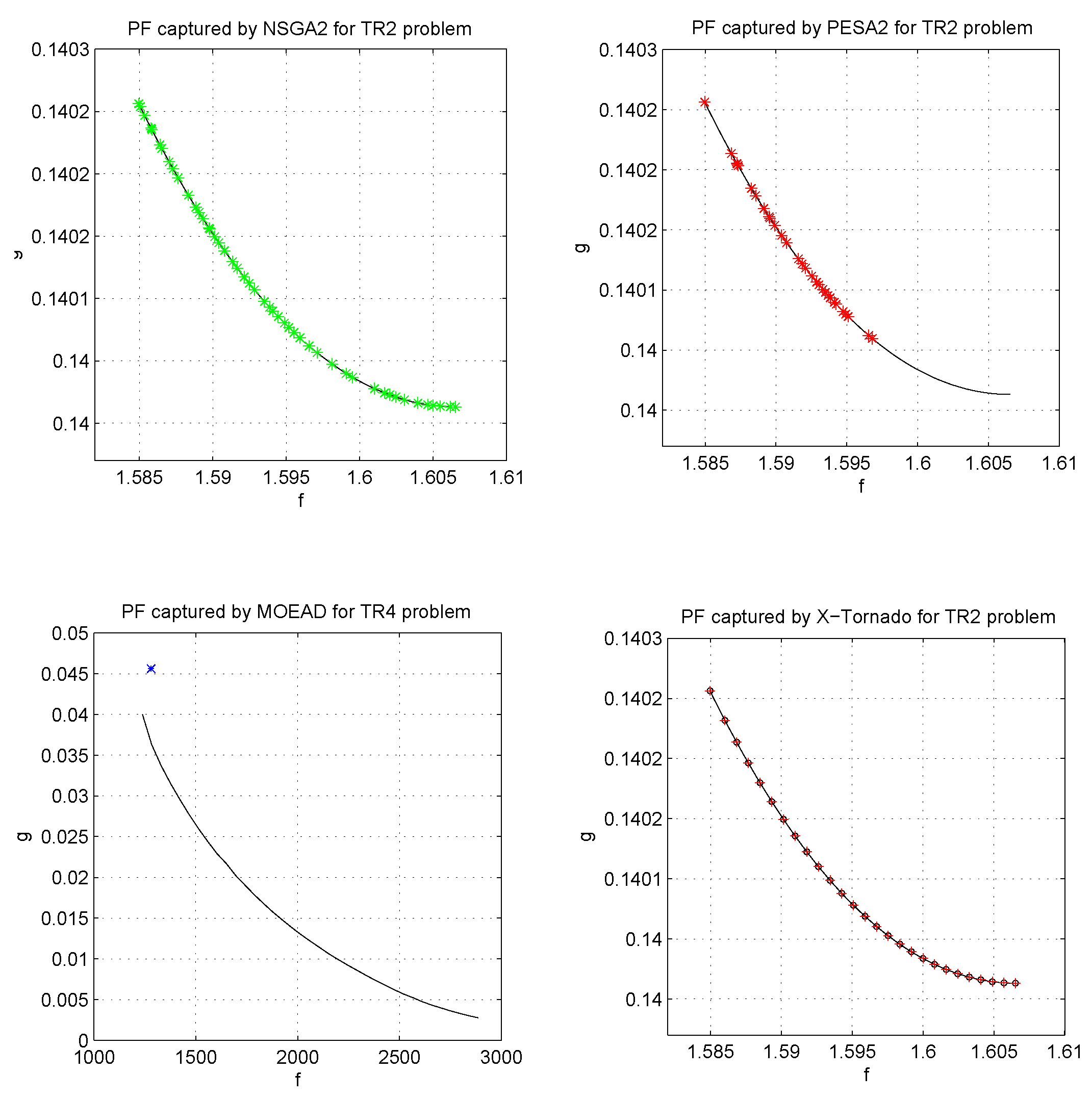
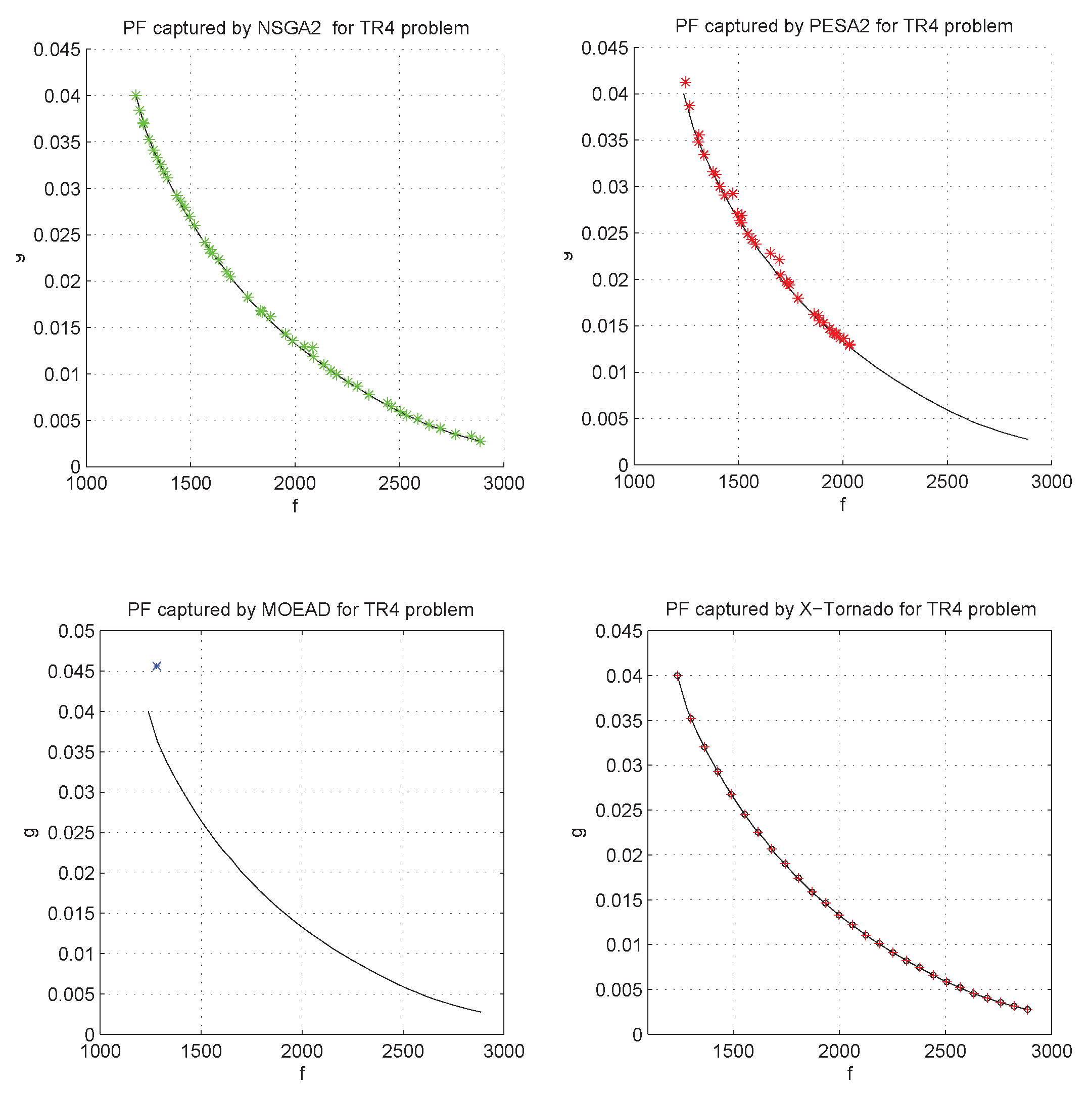
Moreover, the distribution of the non dominated points reflects automatically the regularity of the Tchebychev decomposition and unlike the three other algorithms in comparison, a filtering mechanism such as “crowding” is no longer required in our X-Tornado approach. The consequence of this important advantage is that unlike the other methods in comparison, the capture of the front by the X-Tornado method is more continuous and therefore more precise, as illustrated by the Figure 13, Figure 14 and Figure 15. In addition, the X-Tornado method is much faster (at least 5 times less expensive in CPU time) compared to other methods as we can observe in

Table 9. Mean Time result for the four algorithms on the 14 selected problems.

Method	${\mathit{F}}_1$	${\mathit{F}}_2$	${\mathit{F}}_3$	${\mathit{F}}_4$	${\mathit{F}}_5$	${\mathit{F}}_6$	${\mathit{F}}_7$	${\mathit{F}}_8$	${\mathit{F}}_9$	${\mathit{F}}_{10}$	${\mathit{F}}_{11}$	${\mathit{F}}_{12}$	${\mathit{F}}_{13}$	${\mathit{F}}_{14}$	$\sum {\mathit{T}}_{\mathit{i}}$
ine Nsga2	78	85	79	91	83	83	16	14	14	81	87	79	77	77	1023
Pesa2	77	74	60	35	83	64	157	200	105	78	43	60	96	66	1244
MOEAD	69	49	68	36	153	46	66	74	72	71	67	65	58	76	1042
Xtornado	17	16	17	23	17	14	15	14	15	17	12	17	14	12	233

.

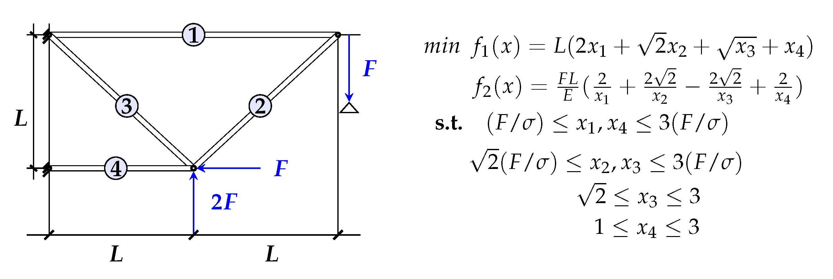
Application to Multi-Objective Structural Optimization Problem

In this section, we consider two applications: The first one is the four bar truss problem proposed by Stadler in [28]. The goal is to find the optimal truss structure while simultaneously minimizing the total mass and static displacement at point C. These two criteria are in conflict since minimizing the mass of a structure tends to increase displacement. So the best solution is to find a trade off between the two criteria. For this, we consider two cost functions to minimize. the total volume ($f_1$ (cm${}^3$))) and displacement ($f_2$ (cm)). The four bar truss problem is shown in Figure 16.

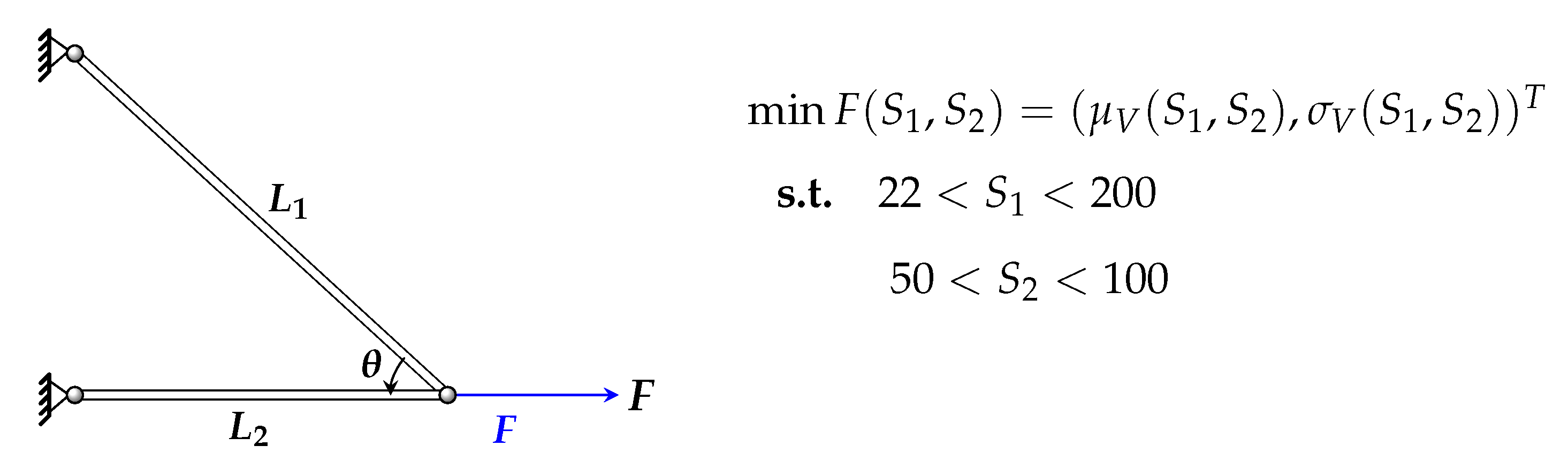
The second application is the two bar truss structure subjected to random Gaussian loading [29]. The two bar problem is a bi-objective problem where the areas of the two bars are decision variables of the optimization. The left end of the bars is fixed while the other end is subjected to a mean plus a fluctuating load. Two objectives are considered for the optimization problem: the mean and the standard deviation of the vertical displacement. Figure 17 illustrates the two bar problem and further technical details can be found in [29].

Table 10. Comparison Results obtained by the four methods for TR4 and TR2 problems.

		GD		Spacing		Spread		CPU(s)
Problem	Method	Mean	Std	Mean	Std	Mean	Std	Mean
ine	Nsga2	$\mathbf{1.49}\times {\mathbf{10}}^{-\mathbf{3}}$	$\mathbf{5.08}\times {\mathbf{10}}^{-\mathbf{5}}$	$\mathbf{1.10}\times {\mathbf{10}}^{+\mathbf{1}}$	$\mathbf{1.06}\times {\mathbf{10}}^{+\mathbf{0}}$	$8.53\times {10}^{-1}$	$9.00\times {10}^{-3}$	$299.0$
TR4	Pesa2	$6.75\times {10}^{-3}$	$1.40\times {10}^{-4}$	$2.19\times {10}^{+1}$	$6.18\times {10}^{+0}$	$9.72\times {10}^{-1}$	$4.37\times {10}^{-2}$	$141.3$
Problem	MOEA/D	$1.44\times {10}^{-2}$	$8.43\times {10}^{-3}$	$2.03\times {10}^{-18}$	$3.52\times {10}^{-18}$	$1.00\times {10}^{+0}$	0	$257.3$
	X-Tornado	$2.27\times {10}^{-3}$	$4.90\times {10}^{-5}$	$1.63\times {10}^{+1}$	$7.36\times {10}^{-1}$	$3.74\times {10}^{-5}$	$5.35\times {10}^{-8}$	$\mathbf{15.8}$
ine	Nsga2	$\mathbf{1.09}\times {\mathbf{10}}^{-\mathbf{3}}$	$\mathbf{2.26}\times {\mathbf{10}}^{-\mathbf{5}}$	$\mathbf{1.45}\times {\mathbf{10}}^{-\mathbf{4}}$	$\mathbf{5.96}\times {\mathbf{10}}^{-\mathbf{6}}$	$9.95\times {10}^{-1}$	$1.23\times {10}^{-4}$	$324.9$
TR2	Pesa2	$7.50\times {10}^{+0}$	$1.98\times {10}^{+0}$	$3.05\times {10}^{-2}$	$8.45\times {10}^{-3}$	$1.09\times {10}^{+0}$	$1.29\times {10}^{-2}$	$189.0$
Problem	MOEA/D	$1.80\times {10}^{-5}$	$9.91\times {10}^{-6}$	$2.14\times {10}^{-3}$	$1.76\times {10}^{-6}$	$1.01\times {10}^{+0}$	$7.62\times {10}^{-6}$	$294.5$
	X-Tornado	$1.94\times {10}^{-3}$	$5.09\times {10}^{-10}$	$1.52\times {10}^{-4}$	$2.45\times {10}^{-11}$	$9.91\times {10}^{-1}$	$1.02\times {10}^{-9}$	$\mathbf{74.6}$

show the comparison results for the four methods in comparisons in term of GD and Spacing metrics for 300,000 Fes. By analysing these results we observe that X-Tornado is performing as well as Nsga2 in term of convergence and spacing metrics and outperforms Pesa2 and MOEA/D for this two problems. Moreover, X-Tornado is much faster in comparison to the three algorithms.

In addition, Figure 18 and Figure 19 illustrate the advantages of X-Tornado PF in term of convergence and regularity over the other comparative algorithms.

5. Conclusions and Future Work

In this paper, we have successfully developed the X-Tornado algorithm which is based on Chaotic search.

The proposed X-Tornado algorithm was tested on various benchmark problems with different features and complexity levels. The results obtained amply demonstrate that the approach is efficient in converging to the true Pareto fronts and finding a diverse set of solutions along the Pareto front. Our approach largely outperforms some popular evolutionary algorithms such as MOEA/D, NSGA-II, and PESA-II in terms of the convergence, cardinality and diversity of the obtained Pareto fronts. The X-Tornado algorithm is characterized by its fast and accurate convergence, and parallel independent decomposition of the objective space.

We are investigating to develop new adaptive mechanism in order to extend X-Tornado to the field of challenging constrained problems involving multi-extremal problems [30,31].

A massively parallel implementation on heterogeneous architectures composed of multi-cores and GPUs is under development. It is obvious that the proposed algorithms have to be improved to tackle many objective optimization problems. We will also investigate the adaptation of the algorithms to large scale MOPs such as the hyperparameter optimization of deep neural networks.

References

1. Pinter, J.D. Global Optimization in Action; Kluwer Academic Publishers: Dordrecht, The Netherlands, 1979. [Google Scholar]
2. Strongin, R.G.; Sergeyev, Y.D. Global Optimization with Non-convex Constraints: Sequential and Parallel Algorithms; Kluwer Academic Publishers: Dordrecht, The Netherlands, 2000. [Google Scholar]
3. Paulavicius, R.; Zilinskas, J. Simplicial Global Optimization; Springer: New York, NY, USA, 2014. [Google Scholar]
4. Talbi, E.G. Metaheuristics: From Design to Implementation; Wiley: Hoboken, NJ, USA, 2009. [Google Scholar]
5. Coello Coello, C.A. Multi-objective optimization. In Handbook of Heuristics; Martí, R., Pardalos, P., Resende, M., Eds.; Springer International Publishing AG: Cham, Switzerland, 2018; pp. 177–204. [Google Scholar]
6. Diehl, M.; Glineur, F.; Jarlebring, E.; Michiels, W. Recent Advances in Optimization and Its Applications in Engineering; Springer: Berlin/Heidelberg, Germany, 2010. [Google Scholar]
7. Battaglia, G.; Di Matteo, A.; Micale, G.; Pirrotta, A. Vibration-based identification of mechanical properties of orthotropic arbitrarily shaped plates: Numerical and experimental assessment. Compos. Part Eng. 2018, 150, 212–225. [Google Scholar] [CrossRef]
8. Di Matteo, A.; Masnata, C.; Pirrotta, A. Simplified analytical solution for the optimal design of Tuned Mass Damper Inerter for base isolated structures. Mech. Syst. Signal Process. 2019, 134, 106337. [Google Scholar] [CrossRef]
9. Jaimes, A.L.; Martınez, S.Z.; Coello Coello, A.C. An introduction to multiobjective optimization techniques. In Optimization in Polymer Processing; Nova Science Publishers: New York, NY, USA, 2011; pp. 29–58. [Google Scholar]
10. Miettinen, K.; Ruiz, F.; Wierzbicki, P. Introduction to Multiobjective Optimization, Interactive Approaches. In Multiobjective Optimization: Interactive and Evolutionary Approaches; Springer: Heidelberg, Germany, 2008; pp. 27–57. [Google Scholar]
11. Liefooghe, A.; Basseur, M.; Jourdan, L.; Talbi, E.G. ParadisEO-MOEO: A Framework for Evolutionary Multi-objective Optimization. In International Conference on Evolutionary Multi-Criterion Optimization; Springer: Berlin/Heidelberg, Germany, 2007; pp. 386–400. [Google Scholar]
12. Qingfu, Z.; Hui, L. MOEA/D: A Multiobjective Evolutionary Algorithm Based on Decomposition. IEEE Trans. Evol. Comput. 2007, 11, 712–731. [Google Scholar] [CrossRef]
13. Gauvain, M.; Bilel, D.; Liefooghe, A.; Talbi, E.G. Shake them all!: Rethinking selection and replacement in MOEA/D. In International Conference on Parallel Problem Solving from Nature; Springer: Berlin/Heidelberg, Germany, 2014; pp. 641–651. [Google Scholar]
14. Li, B.; Jiang, W. Chaos optimization method and its application. J. Control. Theory Appl. 1997, 14, 613–615. [Google Scholar]
15. Wu, L.; Zuo, C.; Zhang, H.; Liu, Z.H. Bimodal fruit fly optimization algorithm based on cloud model learning. J. Soft Comput. 2015, 21, 1877–1893. [Google Scholar] [CrossRef]
16. Yuan, X.; Dai, X.; Zhao, J.; He, Q. On a novel multi-swarm fruit fly optimization algorithm and its application. J. Appl. Math. Comput. 2014, 233, 260–271. [Google Scholar] [CrossRef]
17. Hang, Y.; Wu, L.; Wang, S. UCAV Path Planning by Fitness-Scaling Adaptive Chaotic Particle Swarm Optimization. J. Math. Probl. Eng. 2013, 2013, 147–170. [Google Scholar]
18. Shengsong, L.; Min, W.; Zhijian, H. Hybrid Algorithm of Chaos Optimization and SLP for Optimal Power Flow Problems with Multimodal Characteristic. IEEE Proc. Gener. Transm. Distrib. 2003, 150, 543–547. [Google Scholar] [CrossRef]
19. Tavazoei, M.S.; Haeri, M. An optimization algorithm based on chaotic behavior and fractal nature. J. Comput. Appl. Math. 2007, 206, 1070–1081. [Google Scholar] [CrossRef] [Green Version]
20. Hamaizia, T.; Lozi, R. Improving Chaotic Optimization Algorithm using a new global locally averaged strategy. In Emergent Properties in Natural and Artificial Complex Systems; Springer Science & Business Media: Berlin/Heidelberg, Germany, 2011; pp. 17–20. [Google Scholar]
21. Hamaizia, T.; Lozi, R.; Hamri, N. Fast chaotic optimization algorithm based on locally averaged strategy and multifold chaotic attractor. J. Appl. Math. Comput. 2012, 219, 188–196. [Google Scholar] [CrossRef] [Green Version]
22. Yang, D.; Li, G.; Cheng, G. On the efficiency of chaos optimization algorithms for global optimization. Chaos Solitons Fractals 2007, 34, 1366–1375. [Google Scholar] [CrossRef]
23. Li, B.; Jiang, W. Optimizing complex function by chaos search. J. Cybern. Syst. 1998, 29, 409–419. [Google Scholar]
24. Al-Dhahir, A. The Henon map. Faculty of Applied Mathematics; University of Twente: Enschede, The Netherlands, 1996. [Google Scholar]
25. Ma, X.L.; Zhang, Q.F.; Tian, G.; Yang, J.; Zhu, Z. On Tchebycheff Decomposition Approaches for Multiobjective Evolutionary Optimization. IEEE Trans. Evol. Comput. 1983, 22, 226–244. [Google Scholar] [CrossRef]
26. Lin, W.; Lin, Q.; Zhu, Z.; Li, J.; Chen, J.; Ming, Z. Evolutionary Search with Multiple Utopian Reference Points in Decomposition-Based Multiobjective Optimization. Complex. J. 2019, 2019, 1–22. [Google Scholar] [CrossRef]
27. Steuer, R.E.; Choo, E. An interactive weighted Tchebycheff procedure for multiple objective programming. J. Math. Program. 1983, 26, 326–344. [Google Scholar] [CrossRef]
28. Stadler, W.; Duer, J. Multicriteria optimization in engineering: A tutorial and survy. In Structural Optimization: Status and Future; American institute of Aeronautics and Astronautics: Reston, VA, USA, 1992; pp. 209–249. [Google Scholar]
29. Zidani, H.; Pagnacco, E.; Sampaio, R.; Ellaia, R.; Souza de Cursi, J.E. Multi-objective optimization by a new hybridized method: Applications to random mechanical systems. Eng. Optim. 2013, 45, 917–939. [Google Scholar] [CrossRef]
30. Gaviano, D.E.; Kvasov, D.; Lera, Y.D.; Sergeyev. Software for Generation of Classes of Test Functions with Known Local and Global MINIMA for global Optimization; TOMS 29; ACM: New York, NY, USA, 2003; pp. 469–480. [Google Scholar]
31. Grishagin, V.A.; Israfilov, R.A. Multidimensional Constrained Global Optimization in Domains with Computable Boundaries. In Proceedings of the CEUR Workshop Proceedings, Turin, Italy, 28–29 September 2015; pp. 75–84. [Google Scholar]
Figure 1. Selection of chaotic variables for CGS.
Algorithms 13 00204 g001
Figure 2. Illustration of symmetrisation approach in 2D.
Algorithms 13 00204 g002
Figure 3. Illustration of axial symmetries S θ + D and S θ + H .
Algorithms 13 00204 g003
Figure 4. Generation of chaotic variables by the symmetrization approach in CGS.
Algorithms 13 00204 g004
Figure 5. Illustration of the CLS mechanism.
Algorithms 13 00204 g005
Figure 6. Illustration of exploration aspect in CLS with the zoom dynamic produced by many local search cycles.
Algorithms 13 00204 g006
Figure 7. Selection of symmetric chaotic variables in CLS.
Algorithms 13 00204 g007
Figure 8. Illustration of the generation of N p = 6 symmetric chaotic points in CLS.
Algorithms 13 00204 g008
Figure 9. Illustration of overflow: R η , i > d B ( ω i ) .
Algorithms 13 00204 g009
Figure 10. Illustration of the 10 power zoom via the successive fractional parts.
Algorithms 13 00204 g010
Figure 11. Illustration of the coordinate adaptative local search in CFS.
Algorithms 13 00204 g011
Figure 12. Illustration of Tchebychev decomposition according to the choice of reference points.
Algorithms 13 00204 g012
Figure 13. Pareto Front captured by X-Tornado for problems F 1 F 6 .
Algorithms 13 00204 g013
Figure 14. Pareto Front captured by X-Tornado for problems F 7 F 12 .
Algorithms 13 00204 g014
Figure 15. Pareto Front captured by X-Tornado for problems F 13 F 18 .
Algorithms 13 00204 g015
Figure 16. Four-bar Truss Problem (TR4).
Algorithms 13 00204 g016
Figure 17. Two-bar Truss Problem (TR2).
Algorithms 13 00204 g017
Figure 18. Obtained Pareto fronts by X-Tornado, NSGA-II, MOEA/D and PESA-II for the problem TR2.
Algorithms 13 00204 g018
Figure 19. Obtained Pareto fronts by X-Tornado, NSGA-II, MOEA/D and PESA-II for the problem TR4.
Algorithms 13 00204 g019